Optogenetic LTP Manipulation and Mathematical Modeling to Investigate Value Plasticity of the Instructive Signal in Mice

Materials and reagents

Biological materials

1. C57BL/6J mice (Japan SLC, Inc., Shizuoka, Japan)

Note: Purchase male mice (4–5 weeks old) and house them at 3–5 mice per cage in most experiments.

Reagents

1. AAV1-hSyn-Chronos:GFP (approximately 10¹² vg/mL, UNC Vector Core, North Carolina, USA, https://www.med.unc.edu/vectorcore/in-stock-aav-vectors/boyden/)

2. AAVDJ-Syn-eYFP (approximately 10⁸ gc/μL, Prof. Toshihisa Ohtsuka, University of Yamanashi, Japan)

Note: Store AAVs at -80 °C.

3. Medetomidine hydrochloride (Zenoaq, Fukushima, Japan)

4. Midazolam (Astellas, Tokyo, Japan, catalog number: 4987211762100)

5. Butorphanol tartrate (Meiji Seika Pharma, Tokyo, Japan)

6. Antisedan (Zenoaq, Fukushima, Japan)

Laboratory supplies

1. Hamilton microsyringe (1701RN Neuros Syringe, 33 G, 10 μL, Hamilton Company, Reno, NV, USA)

2. Microsyringe pump (UMP3; UltraMicroPumpII with SYS-Micro4 Controller, UMP2, UMC4, World Precision Instruments, Sarasota, FL, USA)

3. LED cannula unit (470 nm, TeleLCD-B-4.5-250-6.0, Bio Research Center, Tokyo, Japan); fiber diameter: 0.25 mm; fiber length: 4.5 mm; fiber spacing: 6.0 mm

4. TeleTool (Bio Research Center, Tokyo, Japan)

5. Teleopto-receiver (2 g, TeleR-2-P, an infrared-driven wireless LED unit, Bio Research Center, Tokyo, Japan)

Equipment

1. Sound-attenuating box [600 mm (width) × 450 mm (depth) × 650 mm (height)] (O’Hara & Co., Ltd., model: CL-4212C)

2. Chamber for LTP induction [200 mm (width) × 125 mm (depth) × 110 mm (height)] (Context A) (TOYO-LABO Co., Ltd., model: TP-107A)

3. Conditioning chamber [170 mm (width) × 100 mm (depth) × 100 mm (height)] (Context B) (O’Hara & Co., Ltd., model: CL-3002M)

4. Test chamber [170 mm (width) × 100 mm (depth) × 100 mm (height)] (Context C) (O’Hara & Co., Ltd., model: CLT-3002M)

5. Shock generator (O’Hara & Co., Ltd, model: CL-1010C, SGA-2040)

6. Master-8 (A.M.P.I., Jerusalem, Israel)

7. Infrared-driven remote controller (Teleopto remote controller, Bio Research Center, Tokyo, Japan)

8. Camera for behavioral recording (Watec, model: WAT-902B)

Note: Control the infrared-driven remote controller using a Master-8 during in vivo LTP induction experiments. Set the light stimulation parameters on Master-8 as follows: light pulse width, 5 ms; frequency, 40 Hz; stimulation pattern, 2 s ON/3 s OFF.

Software and datasets

1. TimeFZ4 software (O’Hara & Co., Ltd., Tokyo, Japan, requires a license)

2. Prism 9 software (GraphPad Software, La Jolla, CA, requires a license)

3. Python (Python Software, free to use)

4. The code for the estimation of US values has been deposited to Zenodo: https://doi.org/10.5281/zenodo.15598908

Procedure

A. Stereotaxic adeno-associated virus (AAV) injection into the PB, followed by LED cannula implantation to the CeA

1. Fix the anesthetized five-week-old mouse onto a stereotaxic apparatus.

2. Load 0.5 μL of undiluted AAV vector (per hemisphere injection) into a Hamilton microsyringe.

3. Bilaterally microinject the AAV vector into the PB at the following coordinates: 6.4 mm posterior to bregma, 1.25 mm lateral to the midline, and 3.2 mm ventral to the skull surface. Insert the syringe at a 20° anterior-to-posterior angle to avoid superficial arteries (the coordinates were not adjusted for the 20° angle).

4. Control the injection speed at 50 nL/min using a microsyringe pump.

5. After completion of the injection, leave the syringe in place for 10 min before withdrawal.

6. Allow mice to recover and maintain them for more than four weeks to ensure sufficient transgene expression.

7. Stereotactically insert the LED cannula unit to target the central amygdala using TeleTool at the following coordinates: 1.3 mm posterior to bregma, 3.0 mm lateral to the midline, and 4.4 mm ventral to the skull surface.

8. Allow mice to recover for several days before behavioral experiments.

Notes:

1. Prepare the anesthetic solution for surgery by mixing the following reagents with saline: medetomidine hydrochloride (0.75 mg/kg), midazolam (4.0 mg/kg), and butorphanol tartrate (5.0 mg/kg).

2. Administer Antisedan (0.75 mg/kg) dissolved in saline after surgery to facilitate recovery of the mice.

3. Measure the light power at the fiber tip for each LED cannula unit prior to implantation in mice and use units delivering approximately 5–10 mW.

4. After behavioral experiments, fix the mice, prepare coronal brain sections including the PB and CeA, and verify the expression of the AAV vectors (Chronos:GFP or eYFP), as well as the placement of the LED cannula unit.

B. In vivo LTP induction in the PB-CeA pathway

1. Prepare Context A with the following specifications: chamber: TP-107A, 200 mm (width) × 125 mm (depth) × 110 mm (height); shape: rectangle (lid: acrylic board); floor: white bedding; illumination: 200 lux; background noise: 50 dB white noise; odor: none. Place the chamber inside a sound-attenuating box (CL-4212C).

2. Design the LED stimulation program using TimeFZ4 software.

3. Control light delivery using a programmable stimulator (CL-1010C and Master-8).

4. Attach the Teleopto-receiver to the LED cannula unit in each awake mouse immediately before the session begins.

5. Place each mouse into Context A and start the session as follows: baseline period (3 min); stimulation period (7 min, light-pulse width: 5 ms, frequency: 40 Hz, pattern: 2 s ON/3 s OFF).

Notes:

1. Randomly allocate animals to different experimental conditions.

2. Apply blinding during data collection and analysis in behavioral experiments.

3. Perform mouse handling for several days prior to the experiments.

4. Optogenetic stimulation is expected to induce LTP in the PB-CeA pathway by high-frequency activation of Chronos-expressing PB terminals in the CeA.

C. Weak threat conditioning task for detecting enhanced aversive learning via an increase of US signals

1. On the day following in vivo LTP induction, prepare Context B with the following specifications (Figure 1): chamber: CL-3002M, 170 mm (width) × 100 mm (depth) × 100 mm (height); shape: rectangle; wall material: clear acrylic plates; floor: metal grids; illumination: 200 lux; background noise: 60 dB white noise; odor: ethanol. Place the chamber inside a sound-attenuating box (CL-4212C).

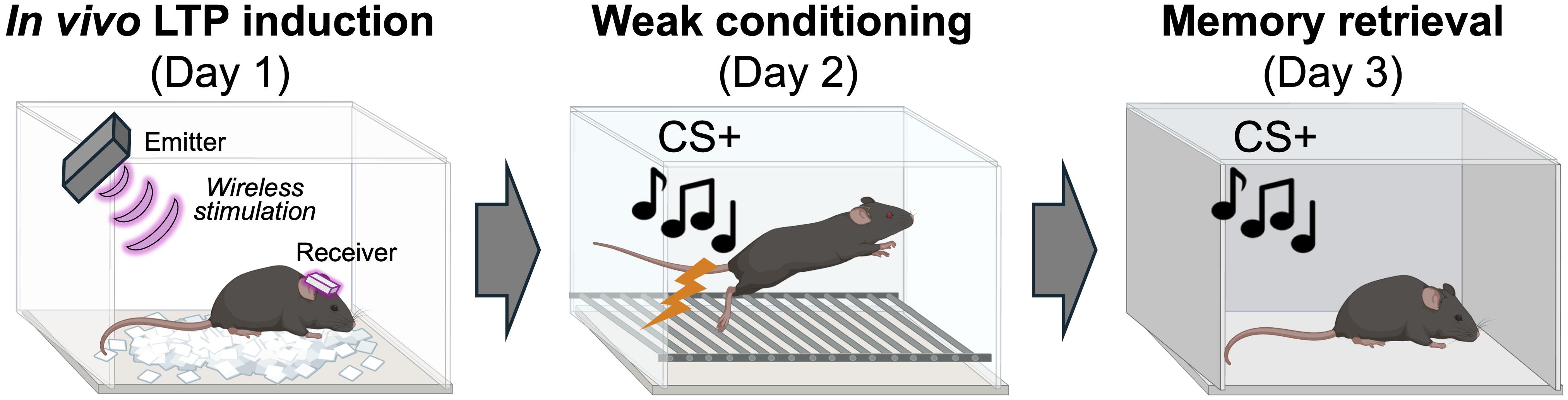
Figure 1. Schematic of the weak threat conditioning task. In vivo long-term potentiation (LTP) induction (section B) is performed by delivering high-frequency optogenetic stimulation using the Teleopto wireless system (Bio Research Center, Tokyo, Japan). Weak conditioning is conducted using conditioned stimulus (CS) (tone) and unconditioned stimulus (US) (foot shock).

2. Design the program using TimeFZ4 software.

3. Control footshock delivery using a programmable stimulator (CL-1010C, SGA-2040).

4. Place each mouse into Context B and start the conditioning session as follows: baseline period (270 s) without stimulation; conditioned stimulus (CS): tone, 10 kHz, 65 dB, 30 s; CS onset times: 270, 440, and 570 s after session start; unconditioned stimulus (US): footshock, 0.1 mA, 2 s; each CS co-terminates with the US.

Note: Prior LTP induction in the PB-CeA pathway is expected to result in enhanced US value of foot shock.

5. On the day following weak threat conditioning, prepare Context C with the following specifications: chamber: CLT-3002M, 170 mm (width) × 100 mm (depth) × 100 mm (height); shape: rectangle; wall material: white acrylic plates; floor: sandpaper; illumination: 200 lux; background noise: 50 dB white noise; odor: peppermint scent. Place the chamber inside a sound-attenuating box (CL-4212C).

6. Place each mouse into Context C and start the retrieval session as follows: baseline period (270 s) without CS presentation; CS: tone, 10 kHz, 65 dB, 30 s; CS onset times: 270, 370, 440, 520, 570, and 660 s after session start; US: not delivered.

Note: Prior LTP induction in the PB-CeA pathway is expected to result in a higher freezing ratio during the retrieval session.

D. Differential threat conditioning task for detecting fear-memory generalization via an increase in US signals

1. On the day following in vivo LTP induction, prepare Context B and design the program using TimeFZ4 software as described above.

2. Place each mouse into Context B and start the conditioning session as follows (Figure 2):

Allow an initial observation period of 270 s without stimulus presentation. Conduct differential threat conditioning using two interleaved auditory CS:

a. CS1 (paired CS): tone type: 4 kHz pure tone; sound level: 65 dB; duration: 30 s; co-terminates with a US footshock (0.3 mA).

b. CS2 (unpaired CS): tone type: 12.5 kHz pulsatile tone; sound level: 65 dB; duration: 30 s; not paired with US footshock.

Present CS1 and CS2 three times each in an interleaved manner according to the following schedule:

CS1 onset times: 270, 440, and 570 s after session start.

CS2 onset times: 370, 520, and 660 s after session start.

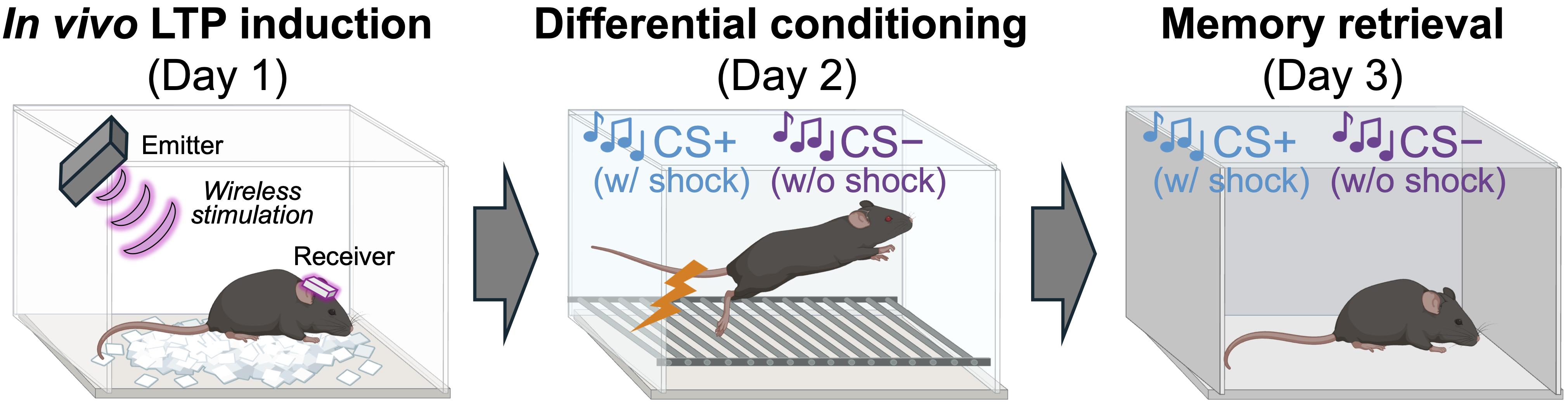
Figure 2. Schematic of the differential threat conditioning task. In vivo long-term potentiation (LTP) induction (section B) is performed by delivering high-frequency optogenetic stimulation using the Teleopto wireless system (Bio Research Center, Tokyo, Japan). Differential conditioning is conducted using CS+ (CS1 tone paired with foot shock), CS− (CS2 tone without foot shock).

3. On the day following the conditioning, place each mouse into Context C and start the retrieval session.

4. Deliver three interleaved presentations of CS1 and CS2 during the retrieval test:

CS2 onset times: 270, 440, and 570 s.

CS1 onset times: 370, 520, and 660 s.

Duration: 30 s per tone.

5. After the final CS1 presentation, allow the mice to remain in Context C for an additional 30 s before terminating the session.

Note: Prior LTP induction in the PB-CeA pathway is expected to increase freezing ratio to CS2 during the retrieval session, indicating that LTP in the PB-CeA pathway promotes generalization of fear memory.

E. Behavioral extinction task for computational modeling

1. Prepare Context B and design the program using TimeFZ4 software as described above.

2. Place each mouse into Context B and start the habituation session as follows (day 1) (Figure 3): baseline period (270 s) without stimulation within a total session time of 720 s; CS: tone, 10 kHz, 65 dB, 30 s; CS onset times: 270, 370, 440, 520, 570, and 660 s after session start; US: not delivered.

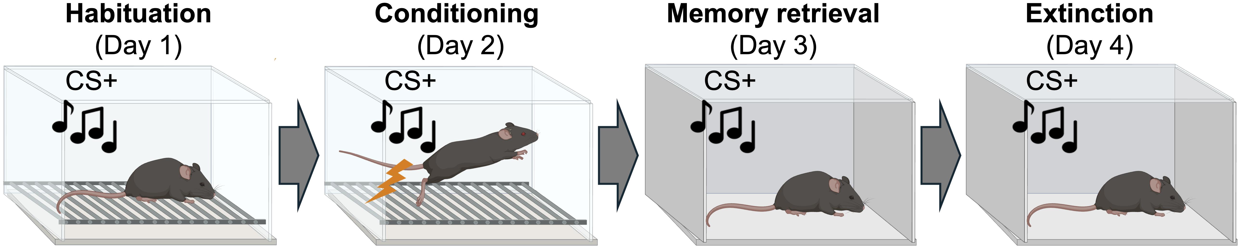
Figure 3. Schematic of the extinction task. The extinction task is conducted using a conditioned stimulus (CS) (tone) and an unconditioned stimulus (US) (foot shock).

3. On the day following the habituation session, perform the conditioning session using Context B as follows (day 2): baseline period (270 s) without stimulation within a total session time of 720 s; CS: tone, 10 kHz, 65 dB, 30 s; CS onset times: 270, 370, 440, 520, 570, and 660 s after session start; US: footshock, 0.3 mA, 2 s; each CS (onset at 270, 440, and 570 s) co-terminates with the US.

4. On the day following the conditioning session, perform the retrieval session using Context C as follows (day 3): baseline period (270 s) without stimulation within a total session time of 720 s; CS: tone, 10 kHz, 65 dB, 30 s; CS onset times: 270, 370, 440, 520, 570, and 660 s after session start; US: not delivered.

5. On the day following the retrieval session, perform the extinction session using Context C as follows (day 4): baseline period (180 s) without stimulation within a total session time of 680 s; CS: tone, 10 kHz, 65 dB, 10 s; CS onset times: 180, 215, 250, 285, 320, 355, 390, 425, 460, 495, 530, 565, 600, 635, and 670 s after session start; US: not delivered.

F. Freezing behavior analysis

1. Record mouse behavior at a sampling rate of 2 frames per second throughout the session.

2. Analyze freezing behavior using TimeFZ4 software.

3. Detect mouse movement by performing pixel-to-pixel subtraction between two consecutive frames.

4. For each frame, behavior was classified as freezing when the total number of pixels showing a detectable frame-to-frame difference was below a predefined threshold.

Critical: Predefined threshold (30 pixels) was pre-optimized by two independent human observers.

5. Calculate the freezing ratio for each tone presentation as follows:

Freezing ratio = (time spent freezing during tone presentation) / (total tone duration)

The freezing ratio ranges from 0 to 1, where 0 indicates no freezing, and 1 indicates continuous freezing.

6. Perform statistical analyses using Prism 9 software.

G. Mathematical model for Bayesian inference of the US value using the Rescorla–Wagner model

1. Describe the model and parameter estimation algorithm using a custom script in Python.

2. Define the Rescorla–Wagner (RW) model for successive threat conditioning as follows:

$w_{n,t}=w_{n,t-1}+\alpha \left(U{S}_{\mathrm{G}\mathrm{r}\mathrm{o}\mathrm{u}\mathrm{p}}-V_{n,t-1}\right)$     (1)

V n , t - 1 = w n , t - 1 C S     (2)

3. Define the model variables and parameters as follows:

α: learning rate, the same value among all mice.

US_Group: value of the US, the same value for the same experimental group of mice.

CS: value of the CS (1 if the mouse received stimulus or 0 if not).

W_n,t: association strength between the US and CS expressed as the synaptic weight in the CS input to the CeA of sample n at time t.

V_n,t: predicted US value, expressed as CeA activity of sample n at time t.

4. Formulate the relationship between the variables of the learning process defined in the RW model and the observable behavioral variable, the freezing ratio.

$z_{n,t}=\tanh \left(V_{n,t}\right)=\frac{\exp \left(V_{n,t}\right)-\exp \left(-V_{n,t}\right)}{\exp \left(V_{n,t}\right)+\exp \left(-V_{n,t}\right)}$     (3)

y n , t = z n , t + σ y E x p ε     (4)

5. Define the model variables and parameters as follows:

z_n,t: mean freezing ratio of sample n at time t.

y_n,t: observed freezing ratio of sample n at time t.

${\sigma }_{\gamma }^{Exp}$: noise strength.

ε: Gaussian noise with zero mean and unit variance.

Exp = {Extinction, Successive Conditioning}

6. Infer the US value for each experimental group (Chronos and eYFP) using a two-step estimation procedure.

7. Directly use the freezing ratio data obtained from the weak threat conditioning task or the extinction task processed under F as y_n,t.

8. In the first step, analyze freezing ratio data obtained during the fear extinction experiment using a separate cohort of mice (extinction group).

9. Assume the US value during fear extinction to be US_Extinction = 0.

10. Assume that the prior distribution of the learning rate (α) follows a beta distribution, as defined below.

$p\left(\alpha \right)=\mathrm{B}\mathrm{e}\mathrm{t}\mathrm{a}\left(\alpha |a,b\right)$     (5)

11. Assume that the prior distribution of the sample-specific initial CS–US association level follows a Gaussian distribution.

$p\left(w_{n,0}\right)=\mathrm{N}\left(w_{n,0}|0,{\sigma }_w^{\mathrm{E}\mathrm{x}\mathrm{t}\mathrm{i}\mathrm{n}\mathrm{c}\mathrm{t}\mathrm{i}\mathrm{o}\mathrm{n}}\right)$     (6)

12. Estimate the learning rate using Markov chain Monte Carlo (MCMC) sampling with the Metropolis–Hastings (M-H) method. Use the mean of the posterior samples to estimate the common learning rate (α) across mice. Set the hyperparameters as follows:

${\sigma }_{\gamma }^{Extinction}$ = 0.1

a = 2

b = 2

${\sigma }_w^{Extinction}$ = 20

13. In the second step, analyze freezing ratio data obtained during the threat conditioning test for each experimental group (Chronos and eYFP). Infer the US value using the learning rate (α) estimated in the first step. Assume that the prior distribution of the US value follows a Gaussian distribution.

$p\left(US\right)=N\left(US|{\mu }_{US},{\sigma }_{US}^2\right)$     (7)

14. Assume that the sample-specific initial CS-US association parameter follows a Gaussian distribution.

$p\left(w_{n,0}\right)=N\left(w_{n,0}|0,{\sigma }_w^{\mathrm{S}\mathrm{u}\mathrm{c}\mathrm{c}\mathrm{e}\mathrm{s}\mathrm{s}\mathrm{i}\mathrm{v}\mathrm{e}\mathrm{ }\mathrm{C}\mathrm{o}\mathrm{n}\mathrm{d}\mathrm{i}\mathrm{t}\mathrm{i}\mathrm{o}\mathrm{n}\mathrm{i}\mathrm{n}\mathrm{g}}\right)$     (8)

15. Perform parameter estimation using MCMC sampling with the M-H method. Set the hyperparameters as follows:

${\sigma }_y^{successive conditioning}$ = 0.01

μ_US = 1

σ²_US = 0.0000001

${\sigma }_w^{successive conditioning}$= 0.1

16. Formulate the Rescorla–Wagner (RW) model to describe CS1-CS2 generalization, as defined below.

$w_{n,t}=w_{n,t-1}+\alpha \left(US-V_{t-1}\right)$     (9)

V n , t = w n , t - 1 C S 1 + w n , t - 1 r C S 2     (10)

$z_{n,t}=\tanh \left(V_{n,t}\right)$     (11)

y n , t = z n , t + σ y E x p ε     (12)

17. Define the model parameters as follows:

CS1: value of CS1 (1 if the mouse received stimulus or 0 if not).

CS2: value of CS2 (same as CS1).

r: generalization parameter.

Other parameters: the same definitions as described above.

18. Directly use the freezing ratio data obtained from the differential threat conditioning task processed under F as y_n,t.

19. Estimate the US parameter using MCMC sampling, employing the same prior distribution as the one used for estimating the US parameter in the standard experiment. Set the hyperparameters as follows:

${\sigma }_y^{successive conditioning}$ = 0.02

μ_US = 6

σ²_US = 0.05

r = 1.5

${\sigma }_w^{successive conditioning}$ = 0.1

20. Perform MCMC sampling using three independent chains. Use one chain to estimate the posterior distributions of parameters. Collect 100,000 samples from the selected chain for parameter estimation. Discard initial samples as burn-in as follows: Discard the first 1,000 samples for the standard experiments. Discard the first 30,000 samples for the CS1-CS2 generalization experiment. For MCMC, regard the chain as having converged when the variability in the sampled values is visually confirmed to be small. Hyperparameters are selected by hand-tuning.

21. Use the remaining two independent chains to assess the reproducibility of parameter estimation.

Validation of protocol

This protocol has been used and validated in the research article [24]. In vivo LTP manipulation in the PB-CeA pathway, an important nociceptive circuit involved in pain processing and emotional learning, was validated to induce synaptic potentiation by an electrophysiological approach using acute brain slices (Figure 1). Following in vivo LTP induction, enhanced aversive learning (eYFP, n = 7; Chronos, n = 8) and increased memory generalization (eYFP, n = 6; Chronos, n = 7) were detected in the weak threat conditioning and differential threat conditioning tasks (Figures 2 and 7). These behavioral experiments were replicated at least once, with consistent results. Although some variability in the data was observed, the use of at least 6–8 mice per group allows for the detection of statistically significant differences. Furthermore, in vivo LTP induction in the PB-CeA pathway resulted in enhanced avoidance behavior (Figure 2) as well as increased shock sensitivity, as assessed by flinching behavior (Supplementary Figure 2). These findings suggest that in vivo LTP induction in the PB-CeA pathway enhances negative US values, supporting the idea that synaptic plasticity within the US pathway updates future learning rules. The US values were further evaluated using a mathematical model based on the behavioral data (the code is available at https://doi.org/10.5281/zenodo.15598908), which revealed that in vivo LTP induction increased the estimated US values (Figure 8 and Supplementary Figure 5).

General notes and troubleshooting

General notes

1. Mice were group-housed (3–5 mice per cage in most experiments) and provided with water and food ad libitum on a 12 h light/dark cycle.

2. In pathway-specific optogenetic approaches for in vivo LTP induction, antidromic activation of other target regions could theoretically occur following stimulation of a single projection target; nevertheless, recent studies indicate that this is not highly likely for projections from the PB region [4,7].

Acknowledgments

The authors would like to thank all the members of the Watabe laboratory for their helpful assistance and Dr. Toshihisa Ohtsuka and Dr. Shun Hamada for providing AAVDJ-Syn-eYFP. This work was supported by the Japan Agency for Medical Research and Development (AMED) Brain Mapping by Integrated Neurotechnologies for Disease Studies (Brain/MINDS) (JP19dm0207081 to A.M.W.), AMED Brain/MINDS 2.0 (JP24wm0625208 to A.M.W.), JSPS Grant-in-Aid for Scientific Research (B) (JP19H04062 and JP22H03542 to A.M.W.), Challenging Research (Exploratory) (JP21K18564 and JP24K21504 to A.M.W.), Scientific Research (C) (JP23K06005 to M.N.), Early-Career Scientists (JP21K16374 and JP24K19295 to T.N.; JP23K16994 to Y.Y.), JST (Moonshot R and D) (JPMJMS2024 to A.M.W. and H.N.), and Cooperative Study Program of Exploratory Research Center on Life and Living Systems (ExCELLS; program number 19-102 to H.N.). The illustrations included in the following figures were created using BioRender: Figure 1, 2, and 3: BioRender.com/csjt1uh. This protocol was used in [24].

Competing interests

The authors declare that they have no competing interests.

Ethical considerations

Behavioral experiments were approved by the Institutional Animal Care and Use Committee of the Jikei University (Tokyo, Japan; Approval No. 2018-072, 2019-045, and 2025-010). Experiments were conducted in accordance with the Guidelines for Proper Conduct of Animal Experiments by the Science Council of Japan (2006) and those recommended by the International Association for the Study of Pain.

References

1. Maren, S. (2001). Neurobiology of Pavlovian fear conditioning. Annu Rev Neurosci. 24: 897–931. https://doi.org/10.1146/annurev.neuro.24.1.897
2. Maren, S. and Fanselow, M. S. (1996). The amygdala and fear conditioning: has the nut been cracked? Neuron. 16(2): 237–240. https://doi.org/10.1016/s0896-6273(00)80041-0
3. Schafe, G. E., Nader, K., Blair, H. T. and LeDoux, J. E. (2001). Memory consolidation of Pavlovian fear conditioning: a cellular and molecular perspective. Trends Neurosci. 24(9): 540–546. https://doi.org/10.1016/s0166-2236(00)01969-x
4. Chiang, M. C., Nguyen, E. K., Canto-Bustos, M., Papale, A. E., Oswald, A.-M. M. and Ross, S. E. (2020). Divergent Neural Pathways Emanating from the Lateral Parabrachial Nucleus Mediate Distinct Components of the Pain Response. Neuron. 106(6): 927–939.e5. https://doi.org/10.1016/j.neuron.2020.03.014
5. Nagase, M., Mikami, K. and Watabe, A. M. (2019). Parabrachial-to-amygdala control of aversive learning. Curr Opin Behav Sci. 26: 18–24. https://doi.org/10.1016/j.cobeha.2018.08.005
6. Palmiter, R. D. (2018). The Parabrachial Nucleus: CGRP Neurons Function as a General Alarm. Trends Neurosci. 41(5): 280–293. https://doi.org/10.1016/j.tins.2018.03.007
7. Bowen, A. J., Chen, J. Y., Huang, Y. W., Baertsch, N. A., Park, S. and Palmiter, R. D. (2020). Dissociable control of unconditioned responses and associative fear learning by parabrachial CGRP neurons. eLife. 9: e59799. https://doi.org/10.7554/eLife.59799
8. Campos, C. A., Bowen, A. J., Roman, C. W. and Palmiter, R. D. (2018). Encoding of danger by parabrachial CGRP neurons. Nature. 555(7698): 617–622. https://doi.org/10.1038/nature25511
9. Han, S., Soleiman, M. T., Soden, M. E., Zweifel, L. S. and Palmiter, R. D. (2015). Elucidating an Affective Pain Circuit that Creates a Threat Memory. Cell. 162(2): 363–374. https://doi.org/10.1016/j.cell.2015.05.057
10. Ito, M., Nagase, M., Tohyama, S., Mikami, K., Kato, F. and Watabe, A. M. (2021). The parabrachial-to-amygdala pathway provides aversive information to induce avoidance behavior in mice. Mol Brain. 14(1): 94. https://doi.org/10.1186/s13041-021-00807-5
11. Kang, S. J., Liu, S., Ye, M., Kim, D.-I., Pao, G. M., Copits, B. A., Roberts, B. Z., Lee, K.-F., Bruchas, M. R. and Han, S. (2022). A central alarm system that gates multi-sensory innate threat cues to the amygdala. Cell Rep. 40(7): 111222. https://doi.org/10.1016/j.celrep.2022.111222
12. Sato, M., Ito, M., Nagase, M., Sugimura, Y. K., Takahashi, Y., Watabe, A. M. and Kato, F. (2015). The lateral parabrachial nucleus is actively involved in the acquisition of fear memory in mice. Mol Brain. 8: 22. https://doi.org/10.1186/s13041-015-0108-z
13. Bird, G. C., Lash, L. L., Han, J. S., Zou, X., Willis, W. D. and Neugebauer, V. (2005). Protein kinase A-dependent enhanced NMDA receptor function in pain-related synaptic plasticity in rat amygdala neurones. J Physiol. 564(Pt 3): 907–921. https://doi.org/10.1113/jphysiol.2005.084780
14. Han, J. S., Bird, G. C. and Neugebauer, V. (2004). Enhanced group III mGluR-mediated inhibition of pain-related synaptic plasticity in the amygdala. Neuropharmacolog. 46(7): 918–926. https://doi.org/10.1016/j.neuropharm.2004.01.006
15. Han, J. S., Fu, Y., Bird, G. C. and Neugebauer, V. (2006). Enhanced group II mGluR-mediated inhibition of pain-related synaptic plasticity in the amygdala. Mol Pain. 2: 18. https://doi.org/10.1186/1744-8069-2-18
16. Han, J. S. and Neugebauer, V. (2004). Synaptic plasticity in the amygdala in a visceral pain model in rats. Neurosci Lett. 361(1–3): 254–257. https://doi.org/10.1016/j.neulet.2003.12.027
17. Ikeda, R., Takahashi, Y., Inoue, K. and Kato, F. (2007). NMDA receptor-independent synaptic plasticity in the central amygdala in the rat model of neuropathic pain. Pain. 127(1–2): 161–172. https://doi.org/10.1016/j.pain.2006.09.003
18. Miyazawa, Y., Takahashi, Y., Watabe, A. M. and Kato, F. (2018). Predominant synaptic potentiation and activation in the right central amygdala are independent of bilateral parabrachial activation in the hemilateral trigeminal inflammatory pain model of rats. Mol Pain. 14: 1744806918807102. https://doi.org/10.1177/1744806918807102
19. Neugebauer, V., Li, W., Bird, G. C., Bhave, G. and Gereau, R. W. (2003). Synaptic plasticity in the amygdala in a model of arthritic pain: differential roles of metabotropic glutamate receptors 1 and 5. J Neurosci Off J Soc Neurosci. 23(1): 52–63. https://doi.org/10.1523/JNEUROSCI.23-01-00052.2003
20. Ren, W. and Neugebauer, V. (2010). Pain-related increase of excitatory transmission and decrease of inhibitory transmission in the central nucleus of the amygdala are mediated by mGluR1. Mol Pain. 6: 93. https://doi.org/10.1186/1744-8069-6-93
21. Shinohara, K., Watabe, A. M., Nagase, M., Okutsu, Y., Takahashi, Y., Kurihara, H. and Kato, F. (2017). Essential role of endogenous calcitonin gene-related peptide in pain-associated plasticity in the central amygdala. Eur J Neurosci. 46(6): 2149–2160. https://doi.org/10.1111/ejn.13662
22. Torres-Rodriguez, J. M., Wilson, T. D., Singh, S., Torruella-Suárez, M. L., Chaudhry, S., Adke, A. P., Becker, J. J., Neugebauer, B., Lin, J. L., Martinez Gonzalez, S., et al. (2024). The parabrachial to central amygdala pathway is critical to injury-induced pain sensitization in mice. Neuropsychopharmacol Off Publ Am Coll Neuropsychopharmacol. 49(3): 508–520. https://doi.org/10.1038/s41386-023-01673-6
23. Watabe, A. M., Ochiai, T., Nagase, M., Takahashi, Y., Sato, M. and Kato, F. (2013). Synaptic potentiation in the nociceptive amygdala following fear learning in mice. Mol Brain. 6: 11. https://doi.org/10.1186/1756-6606-6-11
24. Tohyama, S., Nagashima, T., Higashino, I., Arima-Yoshida, F., Hiyoshi, K., Nagase, M., Yada, Y., Honda, N. and Watabe, A. M. (2025). Aversive experiences induce valence plasticity of instructive signals to change future learning rules in mice. Commun Biol. 8(1): 1002. https://doi.org/10.1038/s42003-025-08367-3
25. Recorla, R. A. and Wagner, A. R. (1972). A theory of Pavlovian conditioning: variations in the effectiveness of reinforcement and nonreinforcement. Class Cond II Curr Res Theory. 64–99.