Expression variability estimation

Overview

A reader requested more info on our protocols for figure2A where we estimate a gene-wise dispersion statistic. The relevant protocols can be found in the Materials and methods subheading: “Expression variability estimation”. While that section provides a sufficient theoretical explanation of the methods, it might be helpful to readers to see some code to see how we implemented this in detail. Here I will implement these methods in R to recreate figure2A. More specifically, I will estimate a gene-wise dispersion statistic using our 39 chimpanzee RNA-seq samples.

Aanalysis

First, load the necessary libraries for this analysis…
 

library(tidyverse)
library(edgeR)
library(MASS)
library(knitr)
library(broom)
 

Next, read in the data from this study. I will read in the pre-processed Chimpanzee RNA-seq gene count-table which we uploaded to GEO GSE151397 as GSE151397_OrthologousExonRawGeneCounts_Chimpanzee.tsv.gz.
 

#Read in Chimpanzee count table data from GEO
temp <- tempfile()
download.file("https://www.ncbi.nlm.nih.gov/geo/download/?acc=GSE151397&format=file&file=GSE151397%5FOrthologousExonRawGeneCounts%5FChimpanzee%2Etsv%2Egz",destfile=temp,method="curl")
d <- read_delim(gzfile(temp), delim='\t', comment = '#')

#Preview the data
d[1:10, 1:10] 

## # A tibble: 10 x 10
##   Geneid  Chr    Start   End     Strand Length `4x0519` `4x373` `476` `4x0025`
##   <chr>   <chr>  <chr>   <chr>   <chr>   <dbl>    <dbl>   <dbl> <dbl>    <dbl>
##  1 ENSG00… 1;1;1  175684;… 176285… -;-;-     707       0       0     0       4
##  2 ENSG00… 1;1;1… 176957;… 177043… +;+;+…   824        8       3    1        6
##  3 ENSG00… 1      186042   186330 -         289        3      0     2        0
##  4 ENSG00… 1      313681   313774 +          94        0      0     0        0
##  5 ENSG00… 1      355180   355274 +          95        0      1     0        0
##  6 ENSG00… 1      355943   356032 +          90        0      0     0        0
##  7 ENSG00… 1      357158   357240 +          83        0      0     0        0
##  8 ENSG00… 1      357510   358497 +         988        0      3     0        0
##  9 ENSG00… 1;1;1… 361286;… 362104… -;-;-…  1291        0       0    2        0
## 10 ENSG00… 1;1;1… 387554;… 387860… +;+;+…   1363      46      73    20      28

Let’s also download Figure2 - supplemental data file1 which contains the dispersion estimates as presented in the paper.

temp <- tempfile()
download.file("https://elifesciences.org/download/aHR0cHM6Ly9jZG4uZWxpZmVzY2llbmNlcy5vcmcvYXJ0aWNsZXMvNTk5MjkvZWxpZmUtNTk5MjktZmlnMi1kYXRhMS12Mi50eHQ-/elife-59929-fig2-data1-v2.txt?_hash=XboGH78RMMQtbWm1%2FNlTc%2BP30zDx8JCQnHHjY%2BSMU0s%3D",destfile=temp,method="curl")
DispersionEstimatesFromPaper <- read_delim(gzfile(temp), delim='\t', comment = '#')

head(DispersionEstimatesFromPaper) 

## # A tibble: 6 x 12
##   gene  HGNC.symbol Chimp.Mean.Expr… Human.Mean.Expr… Chimp.Overdispe…
##   <chr> <chr>                 <dbl>           <dbl>            <dbl>
## 1 ENSG… TNFRSF18               -20.0            -22.7           2.11 
## 2 ENSG… TNFRSF4                -18.8            -19.3           0.620 
## 3 ENSG… SDF4                   -17.3            -17.1           0.0583
## 4 ENSG… B3GALT6                -18.5            -18.7           0.0921
## 5 ENSG… C1QTNF12               -20.2            -21.0           0.943 
## 6 ENSG… UBE2J2                 -19.0            -18.9           0.0832
## # … with 7 more variables: Human.Overdispersion <dbl>,
## #  Chimp.Mean.Adjusted.Dispersion <dbl>, Human.Mean.Adjusted.Dispersion <dbl>,
## #  Chimp.Mean.Adjusted.Dispersion.SE <dbl>,
## #  Human.Mean.Adjusted.Dispersion.SE <dbl>,
## #  InterspeciesDifferential.Mean.Adjusted.Dispersion.P.value <dbl>,
## #   q.value <dbl>
 

Ok, now let’s process the count table to make sure we can arrive at the same dispersion estimates presented in ‘Figure2 - supplemental data file1’.
 

#First make the data more 'tidy' for easier model fitting in R.
d.tidier <- d %>%
  #Drop some unnecessary columns
  dplyr::select(-c("Chr", "Start", "End", "Strand")) %>%
  #Filter for the adequately expressed genes presented in Figure2
  filter(Geneid %in% DispersionEstimatesFromPaper$gene) %>%
  #Make the data more tidy
  gather(key="sample", value="counts", -Geneid, -Length) %>%
  #Add a column for library size
  group_by(sample) %>%
  mutate(LibrarySize=sum(counts)) %>%
  ungroup()

d.tidier %>% head() 

## # A tibble: 6 x 5
##   Geneid          Length sample counts LibrarySize
##  <chr>            <dbl> <chr>   <dbl>       <dbl>
## 1 ENSG00000186891  1363 4x0519     46    50849503
## 2 ENSG00000186827  1565 4x0519    274    50849503
## 3 ENSG00000078808  3750 4x0519   5967    50849503
## 4 ENSG00000176022  2761 4x0519   1097    50849503
## 5 ENSG00000184163  1791 4x0519      7    50849503
## 6 ENSG00000160087  3082 4x0519    761    50849503

Materials and methods subheading: “Expression variability estimation”, the first step in estimating the dispersion statistic is fitting a negative binomial model to the count data for each gene to estimate the mean expression, , and overdispersion, , parameters.

We will use the MASS::glm.nb to accomplish this. In addition to the official documentation for this function, this link (https://www.analytical.unsw.edu.au/sites/default/files/document_related_files/2019April_Seminar_How%20to%20deal%20with%20count%20data_Maslen_1.pdf) is a good primer on fitting count data using this function.

As per the documentation, the MASS:glm function will include estimation of overdispersion, denoted as in the documentation, which corresponds to 1/dispersion paramter in other parameterizations of negative binomial models (in other words, larger theta means less overdispersion compared to Poisson). Also note that MASS:glm.nb uses a log-link function, meaning will correspond to . Also note that we will include an offset of LibrarySize and Length (gene length that is) in the model, meaning that coefficient that we estimate will be analgous to .

There are some nice tidyverse functions that we can make use of to fit this model for each gene in the tidy dataframe we just created.

#First create a function for the fitting a negative binomial model using MASS::glm.nb function, where the underlying model is parameterized by mu and theta
ModelExpression <-function(df) {
  glm.nb(counts ~ 1 + offset(log(LibrarySize))-offset(log(Length)), data=df)
}

#Now create a wrapper function around the modelling function to return NA in case of errors
#This allows purr::map to use my modeling function without breaking the loop when an error happens
ModelExpression.possibly <- possibly(ModelExpression, NA)

#Sample a random gene and fit model to demonstrate
set.seed(0)
MyRandomGene <- sample(d.tidier$Geneid, 1)
print(MyRandomGene)

## [1] "ENSG00000163602"

ExampleFit <- d.tidier %>%
  filter(Geneid==MyRandomGene) %>%
  ModelExpression.possibly

summary(ExampleFit)

## 
## Call:
## glm.nb(formula = counts ~ 1 + offset(log(LibrarySize)) - offset(log(Length)), 
##     data = df, init.theta = 6.511695637, link = log)
## 
## Deviance Residuals: 
##     Min       1Q  Median       3Q      Max 
## -1.6262 -0.8208  -0.2994   0.3023  3.0095  
## 
## Coefficients:
##            Estimate Std. Error z value Pr(>|z|)    
## (Intercept) -18.9996     0.0629 -302.1   <2e-16 ***
## ---
## Signif. codes: 0 '***' 0.001 '**' 0.01 '*' 0.05 '.' 0.1 ' ' 1
## 
## (Dispersion parameter for Negative Binomial(6.5117) family taken to be 1)
## 
##     Null deviance: 40.034  on 38  degrees of freedom
## Residual deviance: 40.034  on 38 degrees of freedom
## AIC: 606.54
## 
## Number of Fisher Scoring iterations: 1
## 
## 
##              Theta:  6.51 
##          Std. Err.:  1.45 
## 
##  2 x log-likelihood:  -602.542

#Now use purr::nest and purr::map to fit models on a loop for each gene and some other purrr functions to extract the info we want.
set.seed(0)
ModelFits <- d.tidier %>%
  group_by(Geneid) %>%
  nest() %>%
  mutate(model = map(data, ModelExpression.possibly),
         tidier = map(model, tidy),
         theta = map_dbl(model, "theta", .default=NA)) %>%
  unnest(tidier, theta)

head(ModelFits) %>% print()

## # A tibble: 6 x 10
## # Groups:  Geneid [6]
##   Geneid   data   model term  estimate std.error statistic p.value x      theta
##  <chr>    <list>  <lis> <chr>    <dbl>     <dbl>     <dbl>   <dbl> <lgl>  <dbl>
## 1 ENSG000… <tibbl… <neg… (Int…    -20.0   0.233      -86.0       0 NA    0.475
## 2 ENSG000… <tibbl… <neg… (Int…    -18.8   0.126     -149.        0 NA    1.61 
## 3 ENSG000… <tibbl… <neg… (Int…    -17.3   0.0387    -445.        0 NA   17.1  
## 4 ENSG000… <tibbl… <neg… (Int…    -18.5   0.0489    -379.        0 NA   10.9  
## 5 ENSG000… <tibbl… <neg… (Int…    -20.2   0.156     -129.        0 NA    1.06 
## 6 ENSG000… <tibbl… <neg… (Int…    -19.0   0.0467    -407.        0 NA   12.0

Ok. That was all the model fitting for each gene. Now let’s do some checks that the results make sense. For example, let’s check across all genes, that the estimated (the intercept coefficent by the way we did this modelling), corresponds to mean log(RPKM).

#Fist calculate log(RPKM)
LogRPKM <- d %>%
  dplyr::select(-c("Chr", "Start", "End", "Strand", "Length")) %>%
  column_to_rownames("Geneid") %>%
  DGEList() %>%
  rpkm(gene.length=d$Length, log=T, prior.count = 0.01)
LogRPKM[1:5,1:5] 

##                    4x0519       4x373        476    4x0025        438
## ENSG00000273443 -11.429274 -11.4292735 -11.429274  -2.690155 -11.429274
## ENSG00000217801 -2.391470  -2.4804343  -6.041402 -2.327253  -3.870749
## ENSG00000237330 -2.291013 -10.1386328  -3.544685 -10.138633 -10.138633
## ENSG00000223823 -8.518296  -8.5182960  -8.518296 -8.518296  -8.518296
## ENSG00000207730 -8.533563  -0.9437507  -8.533563 -8.533563  -8.533563

#Get the sample mean and standard dev log(RPKM)
LogRPKM.SampleSummaryStats <- data.frame(
  Mean.Log.RPKM=apply(LogRPKM, 1, mean),
  Variance=apply(LogRPKM, 1, var)) %>%
  rownames_to_column("Geneid")

head(LogRPKM.SampleSummaryStats) 

##           Geneid Mean.Log.RPKM  Variance
## 1 ENSG00000273443     -6.374516 13.824340
## 2 ENSG00000217801     -3.808030 10.921168
## 3 ENSG00000237330     -6.525440 14.574590
## 4 ENSG00000223823     -8.310962 1.676502
## 5 ENSG00000207730     -7.722262 5.959459
## 6 ENSG00000207607     -7.522928 6.207301

#Plot mean log(RPKM) vs mu-hat
ModelFits %>%
  inner_join(LogRPKM.SampleSummaryStats, by="Geneid") %>%
  ggplot(aes(x=Mean.Log.RPKM, y=estimate)) +
  geom_point() +
  xlab("Sample mean log(RPKM)") +
  ylab("NB fit mu estimate") +
  theme_bw()

Ok, that makes sense. the estimate of expression from the negative binomial fits, , is pretty much proportional to log(RPKM) across all genes. Notice that all the mu values are negative, whereas the logRPKM calculated with edgeR are on a different scale and perhaps shifted so that they are not all negative. Note that the scaling factors in the calculation of logRPKM (eg, Kilobase, per Million reads sequenced), and also the choice of base is arbitrary and explains why there is a shift and rescale transformation between and . If we just do some algeabra to transform the calculated by edgeR (default log base 2, scaling factor of 1/1000 for gene length and 1/1000000 for library size) we can see that and will match up better…

#do some on algebra logRPKM to get rid of the kilo and million scaling factors, and change base to natural log and recalculate sample mean expression so that it should match mu
data.frame(Mean.Log.RPKM=
             log((2**LogRPKM/1E3/1E6)) %>% apply(1, mean)
           ) %>%
  rownames_to_column("Geneid") %>%
  inner_join(ModelFits, by="Geneid") %>%
  ggplot(aes(x=Mean.Log.RPKM, y=estimate)) +
  geom_point() +
  xlab("Sample mean log(RPKM)") +
  ylab("NB fit mu estimate") +
  geom_abline(color="red") +
  theme_bw()

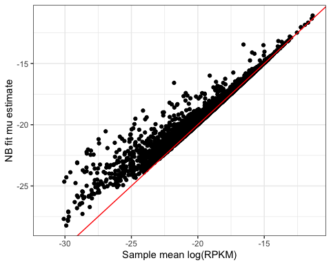
Ok that makes sense. Next let’s check that theta makes sense, in comparison to sample variance(logRPKM). As per documentation for negative binomial models in R (https://cran.r-project.org/web/packages/pscl/vignettes/countreg.pdf), the way this model is paramaterized, variance should be equal to . Note that in the methods section of the paper we refer to overdispersion, , which is , and some some other people use the symbol to refer to the same thing as described in this explanation.

#Check that variance logRPKM roughly corresponds to the variance defined in NB binomial with fitted parameters.
VariancePlot <- ModelFits %>%
  inner_join(LogRPKM.SampleSummaryStats, by="Geneid") %>%
  mutate(ModelVar = estimate + (estimate**2)/theta) %>%
  ggplot(aes(x=Variance, y=ModelVar)) +
  geom_point() +
  xlab("Variance(LogRPKM)") +
  ylab("mu+mu^2/theta") +
  theme_bw()
VariancePlot

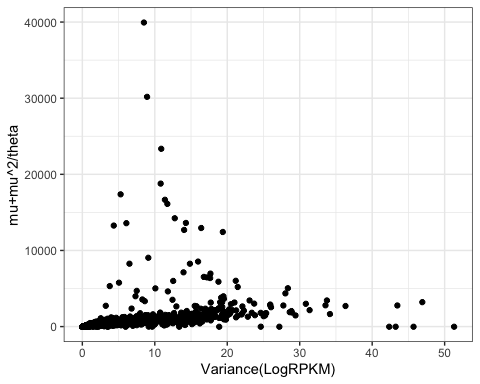
Ok, there are clearly some outlier points, but let’s zoom in on the denser parts of the plot:

VariancePlot +
  ylim(c(0,100)) +
  xlim(c(0,2))

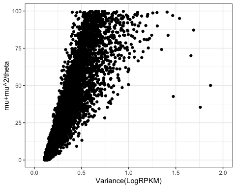
Ok, looks pretty proportional to me. Again, there will be some scaling differences because of choice of log base and scaling factors. But this makes sense.

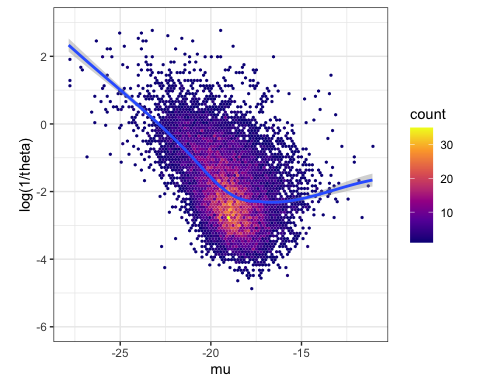
Now let’s make figure2A. In this figure, we show that there is a relationship between overdispersion () and expression (). It is not clear if this is technical or biological, but in any case, in our paper we focus on the component of variability that is independent of expression. So we fit a trend (using loess function) to this relationship, and consider the residual from this trend as a new summary statistic for variability which we refer to as ‘dispersion’.

#plot the loess trend
ModelFits %>%
  ggplot(aes(x=estimate, y=log(1/theta))) +
  stat_binhex(bins=100) +
  ylim(c(-6,3)) +
  xlab("mu") +
  ylab("log(1/theta)") +
  scale_fill_viridis_c(option="C") +
  geom_smooth(method="loess", method.args=list(degree=1)) +
  theme_bw() +
  theme(aspect.ratio = 1)

#assign the loess trend to object
Loess.Trend <- loess(log(1/theta)~estimate, data = ModelFits, degree = 1)

#Add a column for the residual, which we will call 'dispersion'
ModelFits <- ModelFits %>%
  ungroup() %>%
  #Deselect column x and drop rows with na
  #Since the loess trend object drops na values,
  #if I can just use the residuals function to add a column and everything should be in order
  dplyr::select(-x) %>%
  drop_na() %>%
  mutate(Dispersion = residuals(Loess.Trend))

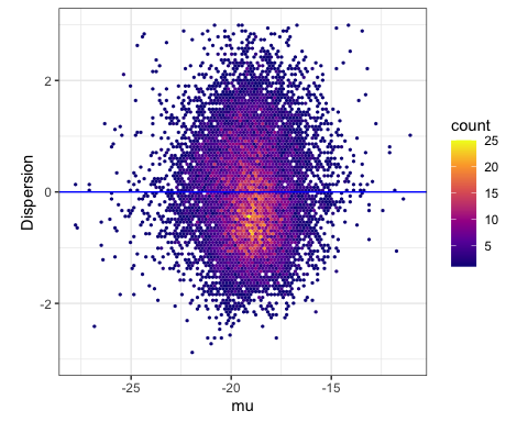
#Plot the residuals, with a horizontal blue line as a way to visually communicate that we are plotting the residuals from the loess trend
ModelFits %>%
  ggplot(aes(x=estimate, y=Dispersion)) +
  stat_binhex(bins=100) +
  ylim(c(-3,3)) +
  xlab("mu") +
  ylab("Dispersion") +
  geom_hline(yintercept =0, color="blue") +
  scale_fill_viridis_c(option="C") +
  theme_bw() +
  theme(aspect.ratio = 1)

Lastly, let’s verify that the dispersion we just calculated, matches with what I published in Figure2 - supplemental data file1. Recall I have already read in this file as a variable DispersionEstimatesFromPaper in one of the first few code chunks.

head(DispersionEstimatesFromPaper) 

## # A tibble: 6 x 12
##   gene  HGNC.symbol Chimp.Mean.Expr… Human.Mean.Expr… Chimp.Overdispe…
##   <chr> <chr>                 <dbl>           <dbl>            <dbl>
## 1 ENSG… TNFRSF18               -20.0            -22.7           2.11 
## 2 ENSG… TNFRSF4                -18.8            -19.3           0.620 
## 3 ENSG… SDF4                   -17.3            -17.1           0.0583
## 4 ENSG… B3GALT6                -18.5            -18.7           0.0921
## 5 ENSG… C1QTNF12               -20.2            -21.0           0.943 
## 6 ENSG… UBE2J2                 -19.0            -18.9           0.0832
## # … with 7 more variables: Human.Overdispersion <dbl>,
## #  Chimp.Mean.Adjusted.Dispersion <dbl>, Human.Mean.Adjusted.Dispersion <dbl>,
## #  Chimp.Mean.Adjusted.Dispersion.SE <dbl>,
## #  Human.Mean.Adjusted.Dispersion.SE <dbl>,
## #  InterspeciesDifferential.Mean.Adjusted.Dispersion.P.value <dbl>,
## #   q.value <dbl>

ModelFits %>%
  dplyr::select(gene=Geneid, Dispersion) %>%
  inner_join(DispersionEstimatesFromPaper) %>%
  ggplot(aes(x=Dispersion, y=Chimp.Mean.Adjusted.Dispersion)) +
  geom_point() +
  ylab("Chimp Dispersion as\npresented in paper") +
  xlab("Chimp Dispersion as\nestimated in this walkthrough") +
  theme_bw()

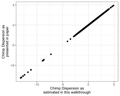
Ok. That looks good!

As described in the Materials and methods subheading: “Expression variability estimation” in the paper, we used a bootstrapping approach (recalculating dispersion after resampling different individuals, repeating for a total of 1000 bootstrap replicates) to estimate standard error in these dispersion estimates, and also to doing differential testing between chimp and human dispersion (requiring 10000 bootstrap replicates with samples randomly drawn from either species to create a null distribution of inter-species differences in dispersion). I won’t be including code to demonstrate those methods in this detailed protocol document because it is pretty computationally intensive to do. For the paper, to accomplish that, I made a script to perform this dispersion calculation from a single bootstrap replicate, then I parrelellized that script across a compute cluster to run many times with random resamples, saving the output to a file for each resample. All code for that and anything else in the paper can be found on a github repo for this paper (but it might be a bit disorganized!).

Category