
- Home
- Protocols

-


Tissue-specific Expression of Target Genes in RiceⅡ(Subcellular Localization and Expression Pattern Analysis)

Last updated date: Nov 16, 2024 DOI: 10.21769/p2759 Views: 215 Forks: 0
 Download PDF
 Ask a
question
Ask a
question
 How to
cite
How to
cite
 Favorite


Background
With the rapid development of high-throughput sequencing technology, whole genome sequencing and the cloning of target genes have become increasingly accessible, making the revelation of gene functions a research goal in the field of plant breeding. This is also an important research focus in the era of functional genomics (post-genomics). Genes are selectively expressed during the growth and development of plants, leading to the differentiation of various organs, with their expression levels varying in different tissues and developmental stages of the individual. Therefore, when studying the function of a gene, we typically need to understand in which organs, tissues, and cells it is expressed, when it is expressed, and how much it is expressed. For analysis based on expression patterns, a variety of semi-quantitative, quantitative, and even visualization techniques have been developed.
Organ and Tissue-Specific Expression: In which organs and tissues is the gene expressed? This can be determined through tissue sectioning and in situ hybridization techniques.
Spatiotemporal Expression Patterns: At which stages of the plant life cycle is the gene expressed? This can be studied by analyzing samples from different developmental stages.
Expression Level Variations: How do the expression levels of the gene change under different conditions? This can be measured using quantitative PCR (qPCR), Northern blotting, and other techniques.
Expression Pattern Analysis Techniques: To analyze gene expression patterns, scientists have developed a variety of techniques, including:
Semi-quantitative Techniques: Such as Northern blotting, which provides relative levels of gene expression.
Quantitative Techniques: Such as qPCR and microarrays, which can precisely measure changes in gene expression levels.
Visualization Techniques: Such as in situ hybridization and histochemical staining of gene expression, which can visually observe gene expression at the cellular or tissue level.
These techniques not only help us understand the role of genes in plant development but also reveal how genes respond to environmental changes and changes in plant physiological status. Through these studies, we can better understand the genetic characteristics of plants, providing a scientific basis for crop improvement and the development of new varieties.
Materials and Reagents
pMDC43 Vector
pGBKT7 Plasmid
KOD FX (for PCR amplification)
rCutSmart Buffer (for restriction enzyme digestion)
ClonExpress Mix (for homologous recombination)
L Enzymatic Hydrolysate I and II (for protoplast extraction)
S Solution (for protoplast transformation)
W Solution (for protoplast transformation)
Asc I-HF
Spe I-HF
2x PCR Buffer
dNTPs (2mM)
PCR Primers (X-F and X-R)
Plant cDNA
DAPI (for DNA staining)
GFP (Green Fluorescent Protein)
PEG 4000 (for transformation)
1 M CaCl2
0.5 M KH2PO4
0.6 M D-Mannitol
Bacterial Strains:
Agrobacterium tumefaciens competent GV3101 cells
LB Medium (for bacterial culture)
Kanamycin and Rifampicin (antibiotics for selection)
MES Buffer (0.2 M)
D-Mannitol Solution (0.6 M)
Acetosyringone (150 mM)
PCR Machine
Agarose Gel Electrophoresis Equipment
Gel Extraction Kit
Centrifuge
Rotary Shaker
Confocal Microscope
Sterile Razor Blade for Sectioning Rice Stems
Additional Reagents:
Bovine Serum Albumin (for L Enzymatic Hydrolysate II)
Celluase R10 and Macerozyme R10 (for L Enzymatic Hydrolysate I)
Subcellular Localization
Note:
The subcellular localization of rice genes is usually achieved by two methods: transformation with protoplasts carrying a recombinant vector of the target gene fused with GFP (or other fluorescent tags), or transformation through Nicotiana benthamiana.
Experimental Procedure
1.Construct pMDC43-X Vector
1.1 PCR Amplification of X Linker Sequence X Sequence Synthesis Rules:
X-F: gcggccgctctagaa + first 20 bp of X CDS
X-R: tgaactatacaaagg + last 20 bp of X CDS (reverse complement)
1.2 Configuration of PCR Amplification System with Linker Gene X (Using KOD FX, TOYOBO KFX-101)
Before preparing the reaction mixture, please thoroughly mix all reagents except for KOD FX (enzyme solution). Frozen reagents should be completely thawed on ice before use.
2x PCR buffer 25 μl
2mM dNTPs 10 μl
X-F Primer 1.5 μl
X-R Primer 1.5 μl
Plant cDNA 0.2 μg
KOD FX (1.0U/μl) 1 μl
ddH2O up to 50 μl Please add KOD FX (enzyme solution) last, and mix the reaction mixture thoroughly with a Vortex or similar device, then spin down before proceeding with PCR.
1.3 PCR Amplification of Gene X with Linkers
Subsequently, use a temperature-controlled PCR machine with the following program:
Predenature 94℃, 2 min.
Denature 98℃, 10 sec
Annealing (Tm-5)℃, 30 sec
Extension 68℃, 1kb/min Set Denature to Extension for 33 cycles.
Final extension 68℃, 7 min. After the reaction is complete, transfer to a 4℃ refrigerator for storage.
1.4 Take the pGBKT7 plasmid out of the -20℃ freezer, place 10x rCutSmart buffer on ice, and after complete dissolution, configure the following system:
10x rCutSmart buffer 5 μl
Asc I-HF 1 μl
Spe I-HF 1 μl
pMDC43 Plasmid DNA 1 μg
ddH2O up to 50 μl Subsequently, use a temperature-controlled PCR machine with the following program:
37℃ 45 min
65℃ 45 sec After the reaction is complete, transfer to a 4℃ refrigerator for storage.
1.5 Agarose Gel Electrophoresis and Gel Recovery (EasyPure Quick Gel Extraction Kit, TransGen Biotech, EG101)
(The method can refer to Wang, S, Huang, Z, Liu, Y, Shao, S, Li, L and Ma, M(2024). Application of the Nicotiana Allergic Necrosis Assay for the Validation of Protein-Protein Interactions between Fungal Effectors and Plant Receptor Kinases. Bio-protocol Preprint. bio-protocol.org/prep2729.)
1.6 Construct pMDC43-X Vector by Homologous Recombination (ClonExpress® Ultra One Step Cloning Kit, Vazyme, C115)
Calculate the dosage of linearized vector and insert fragment:
Optimal cloning vector dosage = [0.02 × cloning vector base pairs] ng (0.03 pmol)
Optimal insert fragment dosage = [0.04 × insert fragment base pairs] ng (0.06 pmol) Note: Calculate the required DNA amount for the recombination reaction according to the formula. To ensure the accuracy of pipetting, dilute the linearized vector and insert fragment appropriately before preparing the recombination reaction system, with each component's volume not less than 1μl. Prepare the following reaction system on ice:
Linearized vector pMDC43 X μl
Insert fragment X μl
2 × ClonExpress Mix 5 μl
ddH2O to 10 μl Gently pipette to mix (do not vortex), briefly centrifuge to collect the reaction liquid at the bottom of the tube. Subsequently, use a temperature-controlled PCR machine with the following program:
50℃ 30 min After the reaction is complete, transfer to a 4℃ refrigerator for storage.
1.7 After sequencing of pMDC43-X, scale up the E. coli culture and extract the plasmid. (The method can refer to Wang, S, Huang, Z, Liu, Y, Shao, S, Li, L and Ma, M(2024). Application of the Nicotiana Allergic Necrosis Assay for the Validation of Protein-Protein Interactions between Fungal Effectors and Plant Receptor Kinases. Bio-protocol Preprint. bio-protocol.org/prep2729.)
2. Agrobacterium Transformation of pMDC43-X Recombinant Plasmid
2.1 Take 5μl of the final pMDC43-X plasmid DNA (approximately 1-2μg) and add it to 100μl of Agrobacterium tumefaciens competent GV3101 cells, then mix well.
2.2 Incubate on ice for 30 minutes, then quickly freeze in liquid nitrogen for 5 minutes, followed by a 37°C water bath for 5 minutes, and immediately place on ice for 2 minutes.
2.3 Add 800μl of liquid LB medium, and culture at 28°C with shaking at 200 rpm for 4 hours.
2.4 Take 200μl of the bacterial culture and spread it on solid LB agar plates containing 50μg/ml Kanamycin and 50 μg/ml Rifampicin, then incubate at 28°C for 48 hours.
3. A buffer formulation and application for efficient protoplast extraction and transformation of rice
3.1. Procure 80 etiolated seedlings of the rice cultivar 9311 that have been cultured in darkness for a period of 12 days. Select the rice stem segment, approximately 5-7 centimeters above the collar of the youngest fully expanded leaf, and prepare it into thin sections with a thickness of 0.4-0.6 millimeters using a sterile, sharp blade—ideally a sterilized razor blade. It is essential that the cutting be executed in a single, swift motion, with a calendered paper placed beneath to facilitate this process. Transfer these thin sections into a 250 milliliter Erlenmeyer flask, ensuring they cover the bottom of the flask.
3.2.Immerse the thin sections in 20 milliliters of L enzyme solution within the flask. To prevent exposure to light, which can adversely affect the enzymatic digestion process, wrap the Erlenmeyer flask with aluminum foil. Incubate the flask on a rotary shaker at a controlled temperature of 28°C Celsius and a shaking speed of 80 revolutions per minute for a duration of four hours. This controlled environment facilitates the enzymatic digestion of the cell walls, thereby releasing the protoplasts from the plant tissue.
3.3.After the cultivation period, the enzymatically treated tissue should be subjected to mechanical filtration through a sieve with a 200-micron mesh size. This step should be performed by gently applying manual pressure to the thin slice fragments to express the protoplasts through the sieve, with meticulous attention to avoid exerting excessive force that could compromise the integrity of the protoplasts.
3.4.The L enzyme solution must be completely drained from the sieve. To facilitate this, a pipette tip, can be utilized to scrape any residual small tissue pieces back into the flask. The initial filtrate, which contains the L enzyme solution, should be discarded, as it no longer serves a purpose in the protocol. The remaining tissue slices, now enriched with isolated protoplasts, should be carefully collected and preserved for subsequent experimental procedures.
3.5. The residual tissue slices obtained after enzymatic digestion should be resuspended in 30 milliliters of S solution. This suspension should then be cultured on a rotary shaker at a speed of 80 revolutions per minute (rpm) in a dark environment maintained at a temperature of 28°C Celsius for a duration of 2 hours. Following this incubation period, the suspension should be passed through a sieve with a mesh size ranging from 100 to 200 microns. The slices will be retained on the sieve, while the liquid fraction is allowed to pass through.
3.6.After the filtration, the slices on the sieve should be washed four times with 5 milliliters of S solution per wash, with each filtrate being collected into a sterile 50 milliliter round-bottom Eppendorf tube. The collected filtrate should then be centrifuged at a speed of 1200 rpm, which corresponds to a centrifugal force of less than 250g, for a period of 6 minutes. The centrifugation process should be conducted with an acceleration and deceleration rate set to 3. Following centrifugation, the supernatant should be carefully removed, and 500 microliters of the precipitate should be retained.
3.7.Subsequently, 500 microliters of S solution should be slowly added along the wall of the 50 ml Eppendorf tube to the retained precipitate. The mixture should then be gently resuspended using a yellow pipette tip, which has been modified by cutting off approximately 0.5 centimeters from the tip and sterilized by flaming for 3 seconds. This results in the formation of the initial suspension solution of 9311 protoplasts, which will appear yellow and turbid, indicating the presence of the isolated protoplasts.
3.8. Prepare a mixture by combining the plasmid DNA, which has been extracted using the Endofree Maxi Plasmid Kit (TIANGEN; China) and has a concentration exceeding 1 ng/μl, with 100 μl of the 9311 protoplast suspension. Subsequently, introduce 110 μl of W solution to the mixture and allow it to incubate on ice for a period of 20 minutes. This step facilitates the interaction between the plasmid DNA and the protoplasts, enhancing the efficiency of subsequent transformation processes.
3.9. Upon completion of the ice incubation, gently add 1 ml of S solution to the reaction mixture along the wall of the container and repetitive invert to ensure thorough mixing. It should be noted that the appearance of small particles under fluorescent light does not significantly impact the experimental outcomes. The mixture is then subjected to centrifugation at 800 rpm for 6 minutes, with the centrifuge acceleration and deceleration settings adjusted to 3. After centrifugation, carefully remove the supernatant. Re-suspend the pellet in 1 ml of S solution, ensuring thorough mixing, and then transfer the suspension to a 28°C incubator for a period of 16 hours in the dark. This dark incubation period is crucial for allowing the protoplasts to recover and for the expression of any introduced genes to occur.
3.10. Following the dark cultivation period, the suspension is centrifuged again at 800 rpm for 6 minutes, with the centrifuge acceleration and deceleration settings maintained at 3. After centrifugation, remove 800 μl of the supernatant to isolate the transformed protoplasts of the experimental group. Gently mix the remaining protoplasts and observe them under a confocal microscope to assess the fluorescence, which serves as an indicator of successful transformation and gene expression. This step is essential for validating the efficiency of the transformation process and for analyzing the outcomes of the introduced genetic material.
Solution formulation
Table 1 L enzymatic hydrolysate I
Reagents name | Measurement (per 100 ml) |
Celluase R10 | 1.0 g |
Macerozyme R10 | 0.5 g |
0.2 M MES | 5 ml |
0.6 M D-Mannitol | to 100 ml |
Note:The formulation of the 0.6 M D-Mannitol solution is shown in Table 2, and the formulation of the 0.2 M MES solution is shown in Table 3.
Table 2 0.6 M D-Mannitol solution
Reagents name | Measurement (per 500 ml) |
D-Mannitol | 54.7 g |
ddH2O | to 500 ml |
Note: Sterilize at 121°C for 15 minutes and store in a 4°C refrigerator for use.
Table 3 0.2 M MES solution
Reagents name | Measurement (per 100 ml) |
| MES | 3.9 g |
| ddH2O | to 100 ml |
Table 4 L enzymatic hydrolysateⅡ
Reagents name | Measurement (per 1000 ml) |
| 1 M CaCl2 | 1000 μL |
| Bovine Serum Albumin | 1 g |
Note: The L enzyme solution I must be freshly prepared to ensure its efficacy. Immediately following preparation, the solution should be subjected to incubation in a water bath maintained at a temperature of 55°C Celsius for a duration of 10 minutes. This step is essential for activating the enzymatic components. After incubation, the solution should be allowed to equilibrate to room temperature.Subsequently, an equal volume of L enzyme solution II should be added to the cooled L enzyme solution I. This mixture yields the final L enzyme solution, which is intended for use in the enzymatic digestion of plant tissues.Prior to its application, the L enzyme solution must be filtered through a 0.22-micrometer filter membrane to remove any potential particulate matter or contaminants. This filtration step is crucial for preventing the introduction of foreign materials into the experimental system, thereby ensuring the purity and reliability of the enzymatic digestion process.
Table 5 S solution
Reagents name | Measurement (per 1000 ml) |
NaCl | 9.0 g |
CaCl2·2H2O | 18.35g |
0.2 M MES | 8 mL |
KCl | 0.447 g |
ddH2O | to 1000mL |
Note: Check if the pH is between 5.56-5.7, if it is lower, adjust the pH to 5.7 using a 1 M KOH solution, sterilize at 121°C for 15 minutes, and then store in a 4°C refrigerator for use.
Table 6 W solution
| Reagents name | Measurement (per 50 ml) |
| PEG 4000 | 20 g |
| 1 M CaCl2 | 5 mL |
| 0.5 M KH2PO4 | 200 ul |
| 0.6 M D-Mannitol | to 50ml |
4.Transient Transformation of Tobacco with Exogenous Proteins containing GFP
Note: Transient transformation can be achieved using either protoplasts or tobacco leaves; transformation via protoplasts can refer to Wang, S, Huang, Z, sijia, T, Feng, S, Liu, X, Shu, Y, Liang, Y and Chen, Z(2024). A buffer formulation and application for efficient protoplast extraction and transformation of rice. Bio-protocol Preprint. bio-protocol.org/prep2723.;while transient transformation using tobacco leaves can refer to Wang, S, Huang, Z, Liu, Y, Shao, S, Li, L and Ma, M(2024). Application of the Nicotiana Allergic Necrosis Assay for the Validation of Protein-Protein Interactions between Fungal Effectors and Plant Receptor Kinases. Bio-protocol Preprint. DOI: 10.21769/p2729.
eg: Transient Transformation of Tobacco Leaves with Exogenous Proteins containing GFP
4.1.1 Inoculation of Agrobacterium Single Colonies:Select single colonies of Agrobacterium containing the final vectors pMDC43-X and inoculate them into 5 ml of LB medium containing 50 μg/ml Kanamycin and 50 μg/ml Rifampicin. Cultivate at 28°C with 200 rpm shaking for 2 days. (Freshly transformed Agrobacterium single colonies can be cultured overnight in 3 ml of medium until day 1.)
4.1.2 Liquid Culture and Expansion: Transfer 1 ml of the cultured Agrobacterium liquid to 20 ml of liquid LB medium containing 50 μg/ml Kanamycin and 50 μg/ml Rifampicin for expanded culture. This LB medium also contains 15 μM acetosyringone. Cultivate at 28°C with 200 rpm shaking until the Agrobacterium reaches the logarithmic growth phase (OD600 = 0.5-0.6).
4.1.3 Collection and Resuspension of Bacterial Cells:Centrifuge at 5,000 rpm for 10 minutes at room temperature to collect the bacterial cells. Resuspend the Agrobacterium cells in infiltration buffer X (containing 10 mM MgCl2, 10 mM MES, 150 μM acetosyringone, pH = 5.6) to an OD600 of 1.0. Allow the cells to stand at room temperature for 2 hours.
4.1.4 Mixture of Bacterial Cultures and Infiltration: Use a 1 ml needle to gently make a small incision on the abaxial side of a Nicotiana benthamiana leaf (be careful not to pierce through). Then, use a needle without a syringe toabsorb the bacterial suspension and inject it into the leaf through the wound. Mark the area on the leaf with a marker.
4.1.5 Cultivation and Phenotypic Observation: Cultivate the injected plants in the dark at approximately 25°C for 48-72 hour, then observe for phenotypes in the areas of the tobacco leaves infiltrated with Agrobacterium, and save photographs using a camera.
Supplementary: Solution Formulas
0.5 M MES (pH 5.6): Weigh out 9.75 g of anhydrous MES and dissolve in deionized water. Adjust the pH to 5.6 with NaOH, bring to a final volume of 100 ml, filter sterilize, and store at 4°C.
150 mM Acetosyringone: Weigh out 2.943g of acetosyringone and dissolve in 5 ml of DMSO (dimethyl sulfoxide). Add deionized water to bring to a final volume of 10 ml, filter sterilize, and store at -20°C.
Note:1 mM=1000 μM
Vector Name: pMDC43
Vector Resistance: Kanamycin, Chloramphenicol
Vector Length: 12460 bp
Vector Type: Gene expression
Replication Origin: ori
Host: Plants
Selection Marker: Hyg
Promoter: CaMV35S (enhanced)
Competent Cells: DB3.1
The forward primer used for sequencing: ggacaggtaatggttgtct
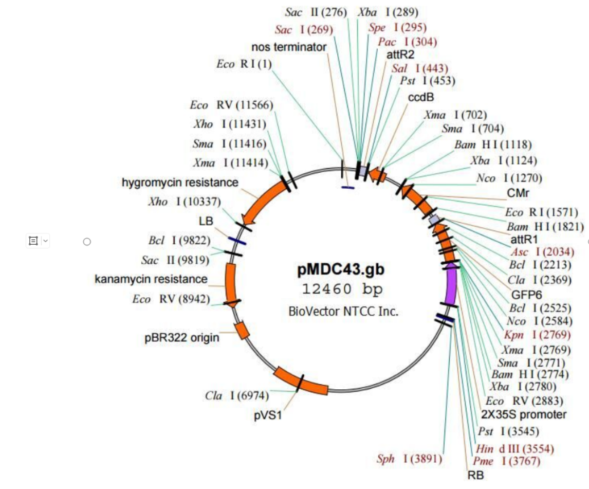
>pMDC43
AATTCAGTAACATAGATGACACCGCGCGCGATAATTTATCCTAGTTTGCGCGCTATATTTTGTTTTCTATCGCGTATTAAATGTATAATTGCGGGACTCTAATCATAAAAACCCATCTCATAAATAACGTCATGCATTACATGTTAATTATTACATGCTTAACGTAATTCAACAGAAATTATATGATAATCATCGCAAGACCGGCAACAGGATTCAATCTTAAGAAACTTTATTGCCAAATGTTTGAACGATCGGGGAAATTCGAGCTCCACCGCGGTGGCGGCCGCTCTAGAACTAGTTAATTAAGAATTATCGAACCACTTTGTACAAGAAAGCTGAACGAGAAACGTAAAATGATATAAATATCAATATATTAAATTAGATTTTGCATAAAAAACAGACTACATAATACTGTAAAACACAACATATCCAGTCACTATGGTCGACCTGCAGACTGGCTGTGTATAAGGGAGCCTGACATTTATATTCCCCAGAACATCAGGTTAATGGCGTTTTTGATGTCATTTTCGCGGTGGCTGAGATCAGCCACTTCTTCCCCGATAACGGAGACCGGCACACTGGCCATATCGGTGGTCATCATGCGCCAGCTTTCATCCCCGATATGCACCACCGGGTAAAGTTCACGGGAGACTTTATCTGACAGCAGACGTGCACTGGCCAGGGGGATCACCATCCGTCGCCCGGGCGTGTCAATAATATCACTCTGTACATCCACAAACAGACGATAACGGCTCTCTCTTTTATAGGTGTAAACCTTAAACTGCATTTCACCAGTCCCTGTTCTCGTCAGCAAAAGAGCCGTTCATTTCAATAAACCGGGCGACCTCAGCCATCCCTTCCTGATTTTCCGCTTTCCAGCGTTCGGCACGCAGACGACGGGCTTCATTCTGCATGGTTGTGCTTACCAGACCGGAGATATTGACATCATATATGCCTTGAGCAACTGATAGCTGTCGCTGTCAACTGTCACTGTAATACGCTGCTTCATAGCACACCTCTTTTTGACATACTTCGGGTATACATATCAGTATATATTCTTATACCGCAAAAATCAGCGCGCAAATACGCATACTGTTATCTGGCTTTTAGTAAGCCGGATCCTCTAGATTACGCCCCGCCCTGCCACTCATCGCAGTACTGTTGTAATTCATTAAGCATTCTGCCGACATGGAAGCCATCACAGACGGCATGATGAACCTGAATCGCCAGCGGCATCAGCACCTTGTCGCCTTGCGTATAATATTTGCCCATGGTGAAAACGGGGGCGAAGAAGTTGTCCATATTGGCCACGTTTAAATCAAAACTGGTGAAACTCACCCAGGGATTGGCTGAGACGAAAAACATATTCTCAATAAACCCTTTAGGGAAATAGGCCAGGTTTTCACCGTAACACGCCACATCTTGCGAATATATGTGTAGAAACTGCCGGAAATCGTCGTGGTATTCACTCCAGAGCGATGAAAACGTTTCAGTTTGCTCATGGAAAACGGTGTAACAAGGGTGAACACTATCCCATATCACCAGCTCACCGTCTTTCATTGCCATACGGAATTCCGGATGAGCATTCATCAGGCGGGCAAGAATGTGAATAAAGGCCGGATAAAACTTGTGCTTATTTTTCTTTACGGTCTTTAAAAAGGCCGTAATATCCAGCTGAACGGTCTGGTTATAGGTACATTGAGCAACTGACTGAAATGCCTCAAAATGTTCTTTACGATGCCATTGGGATATATCAACGGTGGTATATCCAGTGATTTTTTTCTCCATTTTAGCTTCCTTAGCTCCTGAAAATCTCGCCGGATCCTAACTCAAAATCCACACATTATACGAGCCGGAAGCATAAAGTGTAAAGCCTGGGGTGCCTAATGCGGCCGCCATAGTGACTGGATATGTTGTGTTTTACAGTATTATGTAGTCTGTTTTTTATGCAAAATCTAATTTAATATATTGATATTTATATCATTTTACGTTTCTCGTTCAGCTTTTTTGTACAAACTTGTTTGATAGCTTGGCGCGCCTTTGTATAGTTCATCCATGCCATGTGTAATCCCAGCAGCTGTTACAAACTCAAGAAGGACCATGTGGTCTCTCTTTTCGTTGGGATCTTTCGAAAGGGCAGATTGTGTGGACAGGTAATGGTTGTCTGGTAAAAGGACAGGGCCATCGCCAATTGGAGTATTTTGTTGATAATGATCAGCGAGTTGCACGCCGCCGTCTTCGATGTTGTGGCGGGTCTTGAAGTTGGCTTTGATGCCGTTCTTTTGCTTGTCGGCCATGATGTATACGTTGTGGGAGTTGTAGTTGTATTCCAACTTGTGGCCGAGGATGTTTCCGTCCTCCTTGAAATCGATTCCCTTAAGCTCGATCCTGTTGACGAGGGTGTCTCCCTCAAACTTGACTTCAGCACGTGTCTTGTAGTTCCCGTCGTCCTTGAAGAAGATGGTCCTCTCCTGCACGTATCCCTCAGGCATGGCGCTCTTGAAGAAGTCGTGCCGCTTCATATGATCAGGGTAACGGGAGAAGCACTGCACGCCGTAGGTCAGGGTGGTGACCAGGGTTGGCCATGGAACAGGTAGTTTTCCAGTAGTGCAAATAAATTTAAGGGTAAGTTTTCCGTATGTTGCATCACCTTCACCCTCTCCACTGACAGAAAATTTGTGCCCATTAACATCACCATCTAATTCAACAAGAATTGGGACAACTCCAGTGAAAAGTTCTTCTCCTTTACTCATTTTTTCTACCGGTACCCGGGGATCCTCTAGAGTCGAGGTCCTCTCCAAATGAAATGAACTTCCTTATATAGAGGAAGGGTCTTGCGAAGGATAGTGGGATTGTGCGTCATCCCTTACGTCAGTGGAGATATCACATCAATCCACTTGCTTTGAAGACGTGGTTGGAACGTCTTCTTTTTCCACGATGCTCCTCGTGGGTGGGGGTCCATCTTTGGGACCACTGTCGGCAGAGGCATCTTCAACGATGGCCTTTCCTTTATCGCAATGATGGCATTTGTAGGAGCCACCTTCCTTTTCCACTATCTTCACAATAAAGTGACAGATAGCTGGGCAATGGAATCCGAGGAGGTTTCCGGATATTACCCTTTGTTGAAAAGTCTCAATTGCCCTTTGGTCTTCTGAGACTGTATCTTTGATATTTTTGGAGTAGACAAGTGTGTCGTGCTCCACCATGTTATCACATCAATCCACTTGCTTTGAAGACGTGGTTGGAACGTCTTCTTTTTCCACGATGCTCCTCGTGGGTGGGGGTCCATCTTTGGGACCACTGTCGGCAGAGGCATCTTCAACGATGGCCTTTCCTTTATCGCAATGATGGCATTTGTAGGAGCCACCTTCCTTTTCCACTATCTTCACAATAAAGTGACAGATAGCTGGGCAATGGAATCCGAGGAGGTTTCCGGATATTACCCTTTGTTGAAAAGTCTCAATTGCCCTTTGGTCTTCTGAGACTGTATCTTTGATATTTTTGGAGTAGACAAGTGTGTCGTGCTCCACCATGTTGACCTGCAGGCACGCCAAGCTTGGCACTGGCCGTCGTTTTACAACGTCGTGACTGGGAAAACCCTGGCGTTACCCAACTTAATCGCCTTGCAGCACATCCCCCTTTCGCCAGCTGGCGTAATAGCGAAGAGGCCCGCACCGATCGCCCTTCCCAACAGTTGCGCAGCCTGAATGGCGAATGCTAGAGCAGCTTGAGCTTGGATCAGATTGTCGTTTCCCGCCTTCAGTTTAAACTATCAGTGTTTGACAGGATATATTGGCGGGTAAACCTAAGAGAAAAGAGCGTTTATTAGAATAACGGATATTTAAAAGGGCGTGAAAAGGTTTATCCGTTCGTCCATTTGTATGTGCATGCCAACCACAGGGTTCCCCTCGGGATCAAAGTACTTTGATCCAACCCCTCCGCTGCTATAGTGCAGTCGGCTTCTGACGTTCAGTGCAGCCGTCTTCTGAAAACGACATGTCGCACAAGTCCTAAGTTACGCGACAGGCTGCCGCCCTGCCCTTTTCCTGGCGTTTTCTTGTCGCGTGTTTTAGTCGCATAAAGTAGAATACTTGCGACTAGAACCGGAGACATTACGCCATGAACAAGAGCGCCGCCGCTGGCCTGCTGGGCTATGCCCGCGTCAGCACCGACGACCAGGACTTGACCAACCAACGGGCCGAACTGCACGCGGCCGGCTGCACCAAGCTGTTTTCCGAGAAGATCACCGGCACCAGGCGCGACCGCCCGGAGCTGGCCAGGATGCTTGACCACCTACGCCCTGGCGACGTTGTGACAGTGACCAGGCTAGACCGCCTGGCCCGCAGCACCCGCGACCTACTGGACATTGCCGAGCGCATCCAGGAGGCCGGCGCGGGCCTGCGTAGCCTGGCAGAGCCGTGGGCCGACACCACCACGCCGGCCGGCCGCATGGTGTTGACCGTGTTCGCCGGCATTGCCGAGTTCGAGCGTTCCCTAATCATCGACCGCACCCGGAGCGGGCGCGAGGCCGCCAAGGCCCGAGGCGTGAAGTTTGGCCCCCGCCCTACCCTCACCCCGGCACAGATCGCGCACGCCCGCGAGCTGATCGACCAGGAAGGCCGCACCGTGAAAGAGGCGGCTGCACTGCTTGGCGTGCATCGCTCGACCCTGTACCGCGCACTTGAGCGCAGCGAGGAAGTGACGCCCACCGAGGCCAGGCGGCGCGGTGCCTTCCGTGAGGACGCATTGACCGAGGCCGACGCCCTGGCGGCCGCCGAGAATGAACGCCAAGAGGAACAAGCATGAAACCGCACCAGGACGGCCAGGACGAACCGTTTTTCATTACCGAAGAGATCGAGGCGGAGATGATCGCGGCCGGGTACGTGTTCGAGCCGCCCGCGCACGTCTCAACCGTGCGGCTGCATGAAATCCTGGCCGGTTTGTCTGATGCCAAGCTGGCGGCCTGGCCGGCCAGCTTGGCCGCTGAAGAAACCGAGCGCCGCCGTCTAAAAAGGTGATGTGTATTTGAGTAAAACAGCTTGCGTCATGCGGTCGCTGCGTATATGATGCGATGAGTAAATAAACAAATACGCAAGGGGAACGCATGAAGGTTATCGCTGTACTTAACCAGAAAGGCGGGTCAGGCAAGACGACCATCGCAACCCATCTAGCCCGCGCCCTGCAACTCGCCGGGGCCGATGTTCTGTTAGTCGATTCCGATCCCCAGGGCAGTGCCCGCGATTGGGCGGCCGTGCGGGAAGATCAACCGCTAACCGTTGTCGGCATCGACCGCCCGACGATTGACCGCGACGTGAAGGCCATCGGCCGGCGCGACTTCGTAGTGATCGACGGAGCGCCCCAGGCGGCGGACTTGGCTGTGTCCGCGATCAAGGCAGCCGACTTCGTGCTGATTCCGGTGCAGCCAAGCCCTTACGACATATGGGCCACCGCCGACCTGGTGGAGCTGGTTAAGCAGCGCATTGAGGTCACGGATGGAAGGCTACAAGCGGCCTTTGTCGTGTCGCGGGCGATCAAAGGCACGCGCATCGGCGGTGAGGTTGCCGAGGCGCTGGCCGGGTACGAGCTGCCCATTCTTGAGTCCCGTATCACGCAGCGCGTGAGCTACCCAGGCACTGCCGCCGCCGGCACAACCGTTCTTGAATCAGAACCCGAGGGCGACGCTGCCCGCGAGGTCCAGGCGCTGGCCGCTGAAATTAAATCAAAACTCATTTGAGTTAATGAGGTAAAGAGAAAATGAGCAAAAGCACAAACACGCTAAGTGCCGGCCGTCCGAGCGCACGCAGCAGCAAGGCTGCAACGTTGGCCAGCCTGGCAGACACGCCAGCCATGAAGCGGGTCAACTTTCAGTTGCCGGCGGAGGATCACACCAAGCTGAAGATGTACGCGGTACGCCAAGGCAAGACCATTACCGAGCTGCTATCTGAATACATCGCGCAGCTACCAGAGTAAATGAGCAAATGAATAAATGAGTAGATGAATTTTAGCGGCTAAAGGAGGCGGCATGGAAAATCAAGAACAACCAGGCACCGACGCCGTGGAATGCCCCATGTGTGGAGGAACGGGCGGTTGGCCAGGCGTAAGCGGCTGGGTTGTCTGCCGGCCCTGCAATGGCACTGGAACCCCCAAGCCCGAGGAATCGGCGTGACGGTCGCAAACCATCCGGCCCGGTACAAATCGGCGCGGCGCTGGGTGATGACCTGGTGGAGAAGTTGAAGGCCGCGCAGGCCGCCCAGCGGCAACGCATCGAGGCAGAAGCACGCCCCGGTGAATCGTGGCAAGCGGCCGCTGATCGAATCCGCAAAGAATCCCGGCAACCGCCGGCAGCCGGTGCGCCGTCGATTAGGAAGCCGCCCAAGGGCGACGAGCAACCAGATTTTTTCGTTCCGATGCTCTATGACGTGGGCACCCGCGATAGTCGCAGCATCATGGACGTGGCCGTTTTCCGTCTGTCGAAGCGTGACCGACGAGCTGGCGAGGTGATCCGCTACGAGCTTCCAGACGGGCACGTAGAGGTTTCCGCAGGGCCGGCCGGCATGGCCAGTGTGTGGGATTACGACCTGGTACTGATGGCGGTTTCCCATCTAACCGAATCCATGAACCGATACCGGGAAGGGAAGGGAGACAAGCCCGGCCGCGTGTTCCGTCCACACGTTGCGGACGTACTCAAGTTCTGCCGGCGAGCCGATGGCGGAAAGCAGAAAGACGACCTGGTAGAAACCTGCATTCGGTTAAACACCACGCACGTTGCCATGCAGCGTACGAAGAAGGCCAAGAACGGCCGCCTGGTGACGGTATCCGAGGGTGAAGCCTTGATTAGCCGCTACAAGATCGTAAAGAGCGAAACCGGGCGGCCGGAGTACATCGAGATCGAGCTAGCTGATTGGATGTACCGCGAGATCACAGAAGGCAAGAACCCGGACGTGCTGACGGTTCACCCCGATTACTTTTTGATCGATCCCGGCATCGGCCGTTTTCTCTACCGCCTGGCACGCCGCGCCGCAGGCAAGGCAGAAGCCAGATGGTTGTTCAAGACGATCTACGAACGCAGTGGCAGCGCCGGAGAGTTCAAGAAGTTCTGTTTCACCGTGCGCAAGCTGATCGGGTCAAATGACCTGCCGGAGTACGATTTGAAGGAGGAGGCGGGGCAGGCTGGCCCGATCCTAGTCATGCGCTACCGCAACCTGATCGAGGGCGAAGCATCCGCCGGTTCCTAATGTACGGAGCAGATGCTAGGGCAAATTGCCCTAGCAGGGGAAAAAGGTCGAAAAGGTCTCTTTCCTGTGGATAGCACGTACATTGGGAACCCAAAGCCGTACATTGGGAACCGGAACCCGTACATTGGGAACCCAAAGCCGTACATTGGGAACCGGTCACACATGTAAGTGACTGATATAAAAGAGAAAAAAGGCGATTTTTCCGCCTAAAACTCTTTAAAACTTATTAAAACTCTTAAAACCCGCCTGGCCTGTGCATAACTGTCTGGCCAGCGCACAGCCGAAGAGCTGCAAAAAGCGCCTACCCTTCGGTCGCTGCGCTCCCTACGCCCCGCCGCTTCGCGTCGGCCTATCGCGGCCGCTGGCCGCTCAAAAATGGCTGGCCTACGGCCAGGCAATCTACCAGGGCGCGGACAAGCCGCGCCGTCGCCACTCGACCGCCGGCGCCCACATCAAGGCACCCTGCCTCGCGCGTTTCGGTGATGACGGTGAAAACCTCTGACACATGCAGCTCCCGGAGACGGTCACAGCTTGTCTGTAAGCGGATGCCGGGAGCAGACAAGCCCGTCAGGGCGCGTCAGCGGGTGTTGGCGGGTGTCGGGGCGCAGCCATGACCCAGTCACGTAGCGATAGCGGAGTGTATACTGGCTTAACTATGCGGCATCAGAGCAGATTGTACTGAGAGTGCACCATATGCGGTGTGAAATACCGCACAGATGCGTAAGGAGAAAATACCGCATCAGGCGCTCTTCCGCTTCCTCGCTCACTGACTCGCTGCGCTCGGTCGTTCGGCTGCGGCGAGCGGTATCAGCTCACTCAAAGGCGGTAATACGGTTATCCACAGAATCAGGGGATAACGCAGGAAAGAACATGTGAGCAAAAGGCCAGCAAAAGGCCAGGAACCGTAAAAAGGCCGCGTTGCTGGCGTTTTTCCATAGGCTCCGCCCCCCTGACGAGCATCACAAAAATCGACGCTCAAGTCAGAGGTGGCGAAACCCGACAGGACTATAAAGATACCAGGCGTTTCCCCCTGGAAGCTCCCTCGTGCGCTCTCCTGTTCCGACCCTGCCGCTTACCGGATACCTGTCCGCCTTTCTCCCTTCGGGAAGCGTGGCGCTTTCTCATAGCTCACGCTGTAGGTATCTCAGTTCGGTGTAGGTCGTTCGCTCCAAGCTGGGCTGTGTGCACGAACCCCCCGTTCAGCCCGACCGCTGCGCCTTATCCGGTAACTATCGTCTTGAGTCCAACCCGGTAAGACACGACTTATCGCCACTGGCAGCAGCCACTGGTAACAGGATTAGCAGAGCGAGGTATGTAGGCGGTGCTACAGAGTTCTTGAAGTGGTGGCCTAACTACGGCTACACTAGAAGGACAGTATTTGGTATCTGCGCTCTGCTGAAGCCAGTTACCTTCGGAAAAAGAGTTGGTAGCTCTTGATCCGGCAAACAAACCACCGCTGGTAGCGGTGGTTTTTTTGTTTGCAAGCAGCAGATTACGCGCAGAAAAAAAGGATCTCAAGAAGATCCTTTGATCTTTTCTACGGGGTCTGACGCTCAGTGGAACGAAAACTCACGTTAAGGGATTTTGGTCATGCATTCTAGGTACTAAAACAATTCATCCAGTAAAATATAATATTTTATTTTCTCCCAATCAGGCTTGATCCCCAGTAAGTCAAAAAATAGCTCGACATACTGTTCTTCCCCGATATCCTCCCTGATCGACCGGACGCAGAAGGCAATGTCATACCACTTGTCCGCCCTGCCGCTTCTCCCAAGATCAATAAAGCCACTTACTTTGCCATCTTTCACAAAGATGTTGCTGTCTCCCAGGTCGCCGTGGGAAAAGACAAGTTCCTCTTCGGGCTTTTCCGTCTTTAAAAAATCATACAGCTCGCGCGGATCTTTAAATGGAGTGTCTTCTTCCCAGTTTTCGCAATCCACATCGGCCAGATCGTTATTCAGTAAGTAATCCAATTCGGCTAAGCGGCTGTCTAAGCTATTCGTATAGGGACAATCCGATATGTCGATGGAGTGAAAGAGCCTGATGCACTCCGCATACAGCTCGATAATCTTTTCAGGGCTTTGTTCATCTTCATACTCTTCCGAGCAAAGGACGCCATCGGCCTCACTCATGAGCAGATTGCTCCAGCCATCATGCCGTTCAAAGTGCAGGACCTTTGGAACAGGCAGCTTTCCTTCCAGCCATAGCATCATGTCCTTTTCCCGTTCCACATCATAGGTGGTCCCTTTATACCGGCTGTCCGTCATTTTTAAATATAGGTTTTCATTTTCTCCCACCAGCTTATATACCTTAGCAGGAGACATTCCTTCCGTATCTTTTACGCAGCGGTATTTTTCGATCAGTTTTTTCAATTCCGGTGATATTCTCATTTTAGCCATTTATTATTTCCTTCCTCTTTTCTACAGTATTTAAAGATACCCCAAGAAGCTAATTATAACAAGACGAACTCCAATTCACTGTTCCTTGCATTCTAAAACCTTAAATACCAGAAAACAGCTTTTTCAAAGTTGTTTTCAAAGTTGGCGTATAACATAGTATCGACGGAGCCGATTTTGAAACCGCGGTGATCACAGGCAGCAACGCTCTGTCATCGTTACAATCAACATGCTACCCTCCGCGAGATCATCCGTGTTTCAAACCCGGCAGCTTAGTTGCCGTTCTTCCGAATAGCATCGGTAACATGAGCAAAGTCTGCCGCCTTACAACGGCTCTCCCGCTGACGCCGTCCCGGACTGATGGGCTGCCTGTATCGAGTGGTGATTTTGTGCCGAGCTGCCGGTCGGGGAGCTGTTGGCTGGCTGGTGGCAGGATATATTGTGGTGTAAACAAATTGACGCTTAGACAACTTAATAACACATTGCGGACGTTTTTAATGTACTGAATTAACGCCGAATTAATTCGGGGGATCTGGATTTTAGTACTGGATTTTGGTTTTAGGAATTAGAAATTTTATTGATAGAAGTATTTTACAAATACAAATACATACTAAGGGTTTCTTATATGCTCAACACATGAGCGAAACCCTATAGGAACCCTAATTCCCTTATCTGGGAACTACTCACACATTATTATGGAGAAACTCGAGCTTGTCGATCGACAGATCCGGTCGGCATCTACTCTATTTCTTTGCCCTCGGACGAGTGCTGGGGCGTCGGTTTCCACTATCGGCGAGTACTTCTACACAGCCATCGGTCCAGACGGCCGCGCTTCTGCGGGCGATTTGTGTACGCCCGACAGTCCCGGCTCCGGATCGGACGATTGCGTCGCATCGACCCTGCGCCCAAGCTGCATCATCGAAATTGCCGTCAACCAAGCTCTGATAGAGTTGGTCAAGACCAATGCGGAGCATATACGCCCGGAGTCGTGGCGATCCTGCAAGCTCCGGATGCCTCCGCTCGAAGTAGCGCGTCTGCTGCTCCATACAAGCCAACCACGGCCTCCAGAAGAAGATGTTGGCGACCTCGTATTGGGAATCCCCGAACATCGCCTCGCTCCAGTCAATGACCGCTGTTATGCGGCCATTGTCCGTCAGGACATTGTTGGAGCCGAAATCCGCGTGCACGAGGTGCCGGACTTCGGGGCAGTCCTCGGCCCAAAGCATCAGCTCATCGAGAGCCTGCGCGACGGACGCACTGACGGTGTCGTCCATCACAGTTTGCCAGTGATACACATGGGGATCAGCAATCGCGCATATGAAATCACGCCATGTAGTGTATTGACCGATTCCTTGCGGTCCGAATGGGCCGAACCCGCTCGTCTGGCTAAGATCGGCCGCAGCGATCGCATCCATAGCCTCCGCGACCGGTTGTAGAACAGCGGGCAGTTCGGTTTCAGGCAGGTCTTGCAACGTGACACCCTGTGCACGGCGGGAGATGCAATAGGTCAGGCTCTCGCTAAACTCCCCAATGTCAAGCACTTCCGGAATCGGGAGCGCGGCCGATGCAAAGTGCCGATAAACATAACGATCTTTGTAGAAACCATCGGCGCAGCTATTTACCCGCAGGACATATCCACGCCCTCCTACATCGAAGCTGAAAGCACGAGATTCTTCGCCCTCCGAGAGCTGCATCAGGTCGGAGACGCTGTCGAACTTTTCGATCAGAAACTTCTCGACAGACGTCGCGGTGAGTTCAGGCTTTTTCATATCTCATTGCCCCCCGGGATCTGCGAAAGCTCGAGAGAGATAGATTTGTAGAGAGAGACTGGTGATTTCAGCGTGTCCTCTCCAAATGAAATGAACTTCCTTATATAGAGGAAGGTCTTGCGAAGGATAGTGGGATTGTGCGTCATCCCTTACGTCAGTGGAGATATCACATCAATCCACTTGCTTTGAAGACGTGGTTGGAACGTCTTCTTTTTCCACGATGCTCCTCGTGGGTGGGGGTCCATCTTTGGGACCACTGTCGGCAGAGGCATCTTGAACGATAGCCTTTCCTTTATCGCAATGATGGCATTTGTAGGTGCCACCTTCCTTTTCTACTGTCCTTTTGATGAAGTGACAGATAGCTGGGCAATGGAATCCGAGGAGGTTTCCCGATATTACCCTTTGTTGAAAAGTCTCAATAGCCCTTTGGTCTTCTGAGACTGTATCTTTGATATTCTTGGAGTAGACGAGAGTGTCGTGCTCCACCATGTTATCACATCAATCCACTTGCTTTGAAGACGTGGTTGGAACGTCTTCTTTTTCCACGATGCTCCTCGTGGGTGGGGGTCCATCTTTGGGACCACTGTCGGCAGAGGCATCTTGAACGATAGCCTTTCCTTTATCGCAATGATGGCATTTGTAGGTGCCACCTTCCTTTTCTACTGTCCTTTTGATGAAGTGACAGATAGCTGGGCAATGGAATCCGAGGAGGTTTCCCGATATTACCCTTTGTTGAAAAGTCTCAATAGCCCTTTGGTCTTCTGAGACTGTATCTTTGATATTCTTGGAGTAGACGAGAGTGTCGTGCTCCACCATGTTGGCAAGCTGCTCTAGCCAATACGCAAACCGCCTCTCCCCGCGCGTTGGCCGATTCATTAATGCAGCTGGCACGACAGGTTTCCCGACTGGAAAGCGGGCAGTGAGCGCAACGCAATTAATGTGAGTTAGCTCACTCATTAGGCACCCCAGGCTTTACACTTTATGCTTCCGGCTCGTATGTTGTGTGGAATTGTGAGCGGATAACAATTTCACACAGGAAACAGCTATGACCATGATTACG
Expression Pattern Analysis
1.Plant RNA Extraction Using a Kit Method (e.g., RNAsimple Total RNA Extraction Kit, TIANGEN:DP419)
Reagents:
a.Buffer RZ
b.Chloroform
c.Anhydrous Ethanol
d.Protein Removal Liquid RD
e.Wash Liquid RW
f.RNase-Free ddH2O
Equipment:
a.2 mL Centrifuge Tubes
b.RNase-Free Columns CR3 set
c.Homogenizer
d.Centrifuge
e.Laminar Flow Hood
f.UV-Vis Spectrophotometer for measuring OD260/280
2.Plant RNA Extraction
2.1 Sterilize a steel bead by high temperature and pressure, then add it to a 2 mL centrifuge tube free of RNase. Add approximately 0.2 g of plant tissue to be studied. Subsequently, add 1 mL of Buffer RZ and homogenize the sample using a homogenizer.
2.2 Allow the homogenized sample to stand at room temperature for 5 minutes to ensure complete separation of nucleoprotein complexes.
2.3 Centrifuge at 4°C, 12,000 rpm (~13,400×g) for 5 minutes. Transfer the supernatant to a new 1.5mL RNase-free EP tube.
2.4 Add 200 μL of chloroform, cap the tube, and vortex vigorously for 15 seconds. Let the sample stand at room temperature for 3 minutes.
2.5 Centrifuge at 4°C, 12,000 rpm (~13,400×g) for 10 minutes. The sample will separate into three layers: a yellow organic phase, an intermediate layer, and a colorless aqueous phase. RNA is primarily in the aqueous phase, which constitutes approximately 50% of the volume of the lysis buffer RZ used. Transfer the aqueous phase to a new 1.5mL RNase-free EP tube for further processing.
2.6 Slowly add 0.5 volumes of anhydrous ethanol and mix well (a precipitate may form at this stage). Transfer the solution and precipitate to the RNase-Free Columns CR3 set. Centrifuge at 4°C, 12,000 rpm (~13,400×g) for 30 seconds. If the entire solution and mixture cannot be transferred to the RNase-Free Columns CR3 set at once, perform the transfer in two steps, centrifuging for 30 seconds at 4°C, 12,000 rpm (~13,400×g) each time, discarding the waste in the collection tube.
2.6 Add 500 μL of protein removal liquid RD (ensure ethanol has been added prior to use) to the RNase-Free Columns CR3 set. Centrifuge at 4°C, 12,000 rpm (~13,400×g) for 30 seconds and discard the waste. Place the RNase-Free Columns CR3 set into a collection tube.
2.7 Add 500 μL of wash liquid RW (ensure ethanol has been added prior to use) to the adsorption column CR3. Let stand at room temperature for 2 minutes. Centrifuge at 4°C, 12,000 rpm (~13,400×g) for 30 seconds and discard the waste.
2.8 Repeat step 2.7.
2.9 Place the adsorption column into a 2 mL collection tube and centrifuge at 4°C, 12,000 rpm (~13,400×g) for 2 minutes to remove residual liquid.
Note: The purpose of this step is to remove residual wash liquid from the adsorption column. After centrifugation, place the adsorption column at room temperature for a moment or in a laminar flow hood to dry thoroughly.
2.10 Transfer the adsorption column CR3 to a new 1.5 mL centrifuge tube, add 30-100 μL of RNase-Free water, let stand at room temperature for 2 minutes, and centrifuge at 4°C, 12,000 rpm (~13,400×g) for 2 minutes.
2.11 Repeat step 2.10. Measure the concentration (OD260/280 ratio should be between 1.8-2.0) and store at -80°C.
References:
Chomczynski, P., & Sacchi, N. (2006). The single-step method of RNA isolation by acid guanidinium thiocyanate-phenol-chloroform extraction: twenty-something years on. Nature Protocols, 1(2), 581-585.
RNAsimple Total RNA Extraction Kit DP419 User Manual.
3.Synthesis of cDNA (e.g., using PrimeScript™ RT Reagent Kit with gDNA Eraser, Takara: RR047A)
3.1 Genomic DNA Removal Reaction:Prepare the reaction mixture on ice with the following components. To ensure the accuracy of the reaction mixture preparation, prepare the Master Mix in a quantity that is 2 more than the number of reactions, then aliquot into individual reaction tubes, and finally add the RNA sample.
Reagents Volume
5×gDNA Eraser Buffer 2.0 μl
gDNA Eraser 1.0 μl
Total RNA <1μg
RNase Free dH2O up to 10 μl
Subsequently, use a temperature-controlled PCR machine with a program set at 42°C for 2 minutes, and then quickly transfer to ice.
3.2 Reverse Transcription Reaction:Prepare the reaction mixture on ice. To ensure the accuracy of the reaction mixture preparation, prepare the Master Mix in a quantity that is 2 more than the number of reactions, then aliquot 10 μl into each reaction tube. Gently mix and immediately proceed with the reverse transcription reaction.
Reagents Volume
Reaction mixture from Step 3.1 10.0 μl
PrimeScript RT Enzyme Mix I 1.0 μl
RT Primer Mix 4.0 μl
5×PrimeScript Buffer 2(for Real Time) 4.0 μl
RNase Free dH2O 1.0 μl
Total 20 μl
3.3 Subsequently, use a temperature-controlled PCR machine with the following program:
37°C for 30 minutes
85°C for 5 seconds
Afterward, quickly transfer to ice.
3.3The length of the amplification fragment should be between 70-200bp, with shorter fragments having higher amplification efficiency.
3.4Amplification fragments should avoid continuous single base repeats and the formation of secondary structures as much as possible.
3.5Amplification fragments should be preferably designed at the 3' end of the gene.
3.6It is recommended to test the amplification efficiency of the primers, with an amplification efficiency close to 100% ensuring the repeatability of the experiment.
Preparation of Reaction System:
3.7After preparing the cDNA samples and primers, you can prepare the sample table. Generally, each sample will have three replicates, and three replicates of the internal reference gene control will be set up.
Configure the PCR reaction as follows:
cDNA 2 µl
ddH2O 4 µl
Forward primer (2µM) 0.5 µl
Reverse primer (2µM) 0.5 µl
ddH2O 5 µl
SYBR Green I (2x) 12.5 µl
ROX Reference Dye II (50x) 0.5 µl
Total: 25 µl
3.8Running Reaction Program:
Initial denaturation: 95°C for 0:00:10, 1 cycle
Amplification reaction: 95°C for 0:00:05, 60°C for 0:00:34, 40-45 cycles
Dissociation curve: 95°C for 0:00:15
4.qPCR Data Calculation of Relative Gene Expression (-ΔΔCt Method)
When calculating relative gene expression levels from qPCR data, the -ΔΔCt method is a commonly used approach. Here is the specific calculation process:
Calculate ΔCt: For each sample, the ΔCt value is obtained by subtracting the Ct value of the reference gene (usually a housekeeping gene, such as actin) from the Ct value of the target gene. The formula is:

Calculate ΔΔCt: The ΔΔCt value is the difference between the ΔCt value of the experimental group and the average ΔCt value of the control group (or baseline sample). The formula is:

Calculate 2^(-ΔΔCt): Finally, substitute the ΔΔCt value into the formula to calculate 2^(-ΔΔCt), which gives the relative expression level. The formula is:

Example calculation process:
Suppose we have three samples, a control group (Control) and two experimental groups (Sample1 and Sample2), with the target gene being 595 and the reference gene being actin. The Ct values are as follows:
Control: 595 Ct = 25, actin Ct = 20
Sample1: 595 Ct = 28, actin Ct = 21
Sample2: 595 Ct = 30, actin Ct = 22
First, calculate ΔCt:
ΔCt(Control) = 25 - 20 = 5
ΔCt(Sample1) = 28 - 21 = 7
ΔCt(Sample2) = 30 - 22 = 8
Next, calculate ΔΔCt:
ΔΔCt(Sample1) = 7 - 5 = 2
ΔΔCt(Sample2) = 8 - 5 = 3
Finally, calculate 2^(-ΔΔCt):
Relative Expression(Sample1) = 2^(-2) ≈ 0.25
Relative Expression(Sample2) = 2^(-3) ≈ 0.125
This means that the expression level of the target gene in Sample1 is 0.25 times that of the control group, and in Sample2, it is 0.125 times that of the control group. Using this method, we can compare the relative expression levels of the target gene in different samples.
Note: To investigate the expression patterns in response to external environmental stimuli, the materials used are rice seedlings that have grown for 21 days to the stage of having three leaves and one heart leaf. Add GA (10μM), ABA (100 μM), and JA (100μM) to their nutrient solution and measure the expression levels at 0 h, 1 h, 3 h, 6 h, 12 h, 24 h, 48 h, and 72 h. Similarly, measure the expression levels after treatment with H2O2 (20 mM), PEG (20%), and NaCl (150 mM) at the same time points. UBQ is used as the reference gene. Other steps are the same as for expression pattern analysis.
References:
For a detailed understanding of the methodology and application of the PrimeScript™ RT Reagent Kit with gDNA Eraser, please refer to the following:
1. Takara Bio Inc. (2019). PrimeScript™ RT Reagent Kit with gDNA Eraser. Technical Manual. [Accessed on:2024.10.1]
Reference
Wang, S., Huang, Z., Liu, Y., Shao, S., Li, L., & Ma, M. (2024). Application of the Nicotiana Allergic Necrosis Assay for the Validation of Protein-Protein Interactions between Fungal Effectors and Plant Receptor Kinases. Bio-protocol Preprint. https://doi.org/10.21769/p2729.
Wang, S., Huang, Z., Siji, T., Feng, S., Liu, X., Shu, Y., Liang, Y., & Chen, Z. (2024). A buffer formulation and application for efficient protoplast extraction and transformation of rice. Bio-protocol Preprint. https://doi.org/10.21769/prep2723.
Horsch, R. B., Fry, J. E., Hoffmann, N. L., Eichholtz, D., Rogers, S. G., & Fraley, R. T. (1985). A simple and general method for transferring genes into plants. Science, 227(4691), 1229-1231.
Murashige, T., & Skoog, F. (1962). A revised medium for rapid growth and bio assays with tobacco tissue cultures. Physiologia Plantarum, 15(3), 473-497.
Chalfie, M., Tu, Y., Euskirchen, G., Ward, W. W., & Prasher, D. C. (1994). Green fluorescent protein as a marker for gene expression. Science, 263(5148), 802-805.
Sparkes, I. A., Runions, J., Kearns, A., & Hawes, C. (2006). Rapid, transient expression of fluorescent fusion proteins in tobacco plants and generation of stably transformed plants. Nature Protocols, 1(3), 2019-2025.
De Block, M., Herrera-Estrella, L., Van Montagu, M., Schell, J., & Zambryski, P. (1984). Expression of foreign genes in regenerated plants and their progeny. EMBO Journal, 3(7), 1681-1687.
Gamborg, O. L., Miller, R. A., & Ojima, K. (1968). Nutrient requirements of suspension cultures of soybean root cells. Experimental Cell Research, 50(1), 151-158.
Gelvin, S. B. (2000). Agarose gel for DNA and small RNA analysis. In Current Protocols in Molecular Biology (pp. A.3D.1-A.3D.7). John Wiley & Sons.
Sambrook, J., & Russell, D. W. (2001). Molecular Cloning: A Laboratory Manual (3rd ed.). Cold Spring Harbor Laboratory Press.
Results interpretation:
1.
The set of microscope images you provided appears to illustrate the morphological changes in the leaves and trapping structures of the bladderwort plant (Utricularia graminifolia) at various developmental stages, along with the expression patterns of the UgPHV1 and UgFIL1 genes.
Image Analysis:
Panels A-D: Show the development of leaves from young (Lo) to mature (Lt). These images may reveal changes in gene expression corresponding to the maturation of the leaves.
Panels E-H: Display the development of the trapping structures from young (LI) to mature (Tt). These images likely show the relationship between gene expression and the morphological changes in the traps.
Panels I-J: May provide a detailed look at the internal structure of the trapping structures, showing the reticulated pattern inside the traps.
Panels K-T: Further illustrate the development of the trapping structures, including the formation of the trap door (Tl) and the maturation of the traps.
Panels U-V: Likely offer additional insights into the internal structure of the traps, showing detailed morphology.
Panels W-Y: These images may use different staining techniques to highlight specific structures or gene expression patterns within the traps.
Gene Expression Patterns:
UgPHV1 and UgFIL1: The expression of these genes might be indicated by color changes (such as brown or purple) in the microscope images. The intensity and distribution of the color can reflect the level and location of gene expression.
Expression Patterns: Gene expression might be more pronounced in specific regions or at particular stages of trap development. For instance, if the formation of the trap door (Tl) is associated with these genes, strong expression signals might be observed during specific stages of trap development.
Conclusions:
Developmental Stages: The images show the progression from young to mature stages of both leaves and trapping structures.
Gene Function: UgPHV1 and UgFIL1 genes may play significant roles in the development of the trapping structures, particularly in the formation of the trap door and the maturation of the traps.
Expression Patterns: The patterns of gene expression are likely closely related to the morphological changes in the trapping structures, especially during the formation of the trap door and the maturation stages.
For a more accurate analysis, additional context would be necessary, such as quantitative data on gene expression, detailed descriptions of the staining methods used, and known functions of these genes in bladderwort. Furthermore, these images would benefit from comparison with unstained control images to confirm that the observed signals are indeed due to gene expression.
2.
The results of a GUS (β-glucuronidase) staining assay, which is commonly used to visualize the expression of a gene in plants. The GUS gene is a reporter gene that, when expressed, produces an enzyme that breaks down a colorless substrate into a blue product, which can be easily visualized. Here's an analysis of the results:
General Observations:
Positive Control: The images labeled with "gARF8::GUS" likely represent a positive control where the GUS gene is under the control of a promoter that is known to be active, resulting in blue staining.
Negative Control: The images labeled with "mARF8::GUS" might represent a negative control where the GUS gene is under the control of a promoter that is not expected to be active, resulting in little to no blue staining.
Experimental Groups: The images labeled with "Pwur1187::GUS" and "Pwur1874::GUS" show the expression of the GUS gene under the control of different promoters, which are likely associated with the genes being studied.
Detailed Analysis:
Panels A-J: These panels show the GUS staining in various parts of the plant, including leaves, stems, and roots. The blue color indicates areas where the GUS gene is being expressed. The intensity and distribution of the blue color can give insights into the spatial and temporal expression patterns of the gene.
Panels K-T: These panels focus on the GUS staining in the roots and root hairs. The presence of blue staining in the root hairs suggests that the gene is expressed in these structures, which could be important for processes like nutrient uptake or symbiotic interactions.
Panels U-Y: These panels show the GUS staining in the flowers and developing seeds. The blue color in these structures indicates that the gene is expressed during the reproductive phase of the plant, which could be related to processes like pollination, fertilization, or seed development.
Conclusions:
Expression Patterns: The GUS staining provides a visual representation of where and when the gene of interest is being expressed within the plant.
Functional Insights: The expression patterns can give clues about the potential functions of the gene. For example, if a gene is highly expressed in the roots, it might be involved in root development or interactions with the soil environment.
Comparative Analysis: By comparing the GUS staining patterns of different promoters, researchers can infer the regulatory elements that control gene expression in different tissues or under different conditions.
3.
Columns:
AthHSBP-GFP: This column shows the localization of the AthHSBP protein fused with GFP. The green fluorescence indicates the presence and location of the AthHSBP-GFP fusion protein within the cells.
DAPI: This column shows the staining of the cell nucleus with DAPI, a DNA-binding dye that fluoresces blue upon binding. This is used as a reference for the position of the nucleus.
Chlorophyll: This column shows the auto-fluorescence of chlorophyll, which appears red. This is used to visualize the chloroplasts, the organelles responsible for photosynthesis.
Merge: This column shows the merged images of the three channels, allowing for the visualization of the relative localization of the AthHSBP-GFP fusion protein, the nucleus, and the chloroplasts.
Rows:
CK (Control): The first row serves as a control, showing the normal localization of the AthHSBP-GFP fusion protein in the absence of any treatment or genetic modification.
H1R0, H1R1, H1R2: These rows likely represent different genetic backgrounds or mutants where the AthHSBP gene has been modified or is not functioning properly. The changes in GFP fluorescence pattern compared to the control can indicate the effect of these modifications on the protein's localization.
Observations:
CK: In the control, the AthHSBP-GFP fusion protein is localized around the nucleus and within the chloroplasts, as shown by the overlap of green fluorescence with the blue DAPI staining and red chlorophyll auto-fluorescence.
H1R0, H1R1, H1R2: In these rows, the pattern of GFP fluorescence is altered compared to the control. This could indicate a change in the subcellular localization of the AthHSBP protein due to the genetic modifications. For example, if the green fluorescence is no longer overlapping with the red chlorophyll fluorescence, it might suggest that the protein is no longer being targeted to the chloroplasts.
Conclusions:
The subcellular localization of AthHSBP-GFP is affected in the H1R0, H1R1, and H1R2 backgrounds compared to the control.
The changes in GFP fluorescence patterns can provide insights into how the genetic modifications impact the protein's function and its ability to localize to specific organelles.
Further analysis would be needed to determine the exact nature of the mutations in H1R0, H1R1, and H1R2 and how they affect the AthHSBP protein's localization and function.
4.
Panel A: Graphs
Graphs: These line graphs show the relative expression levels of various genes (e.g., PEC, HAP5, Cor15, SnRK2) under different treatments (e.g., DTT, NaCl, ABA, GA, PAC, IAA, JA). The treatments are likely different stress conditions or hormones.
X-Axis: Represents time points or different concentrations of the treatments.
Y-Axis: Represents the relative expression levels of the genes, which are normalized to a control gene (usually actin or tubulin).
Red and Blue Lines: May represent two different conditions or replicates (e.g., wild type vs. mutant, treated vs. control).
Panel B: Bar Graph
Bar Graph: Shows the relative expression levels of a gene under various abiotic stresses (e.g., osmotic, salinity, drought, heat, cold, H2O2, plum, smoke, wounding, biotic, and pathogen).
Y-Axis: Represents the relative expression levels.
Bars: Each bar represents the expression level under a specific stress condition.
Panel C-G: Photographs of Plants
Panel C: Shows a close-up of a plant part, possibly highlighting a symptom or feature related to the study.
Panel D: Displays a heat map or a graphical representation of data, which could be related to gene expression or physiological responses.
Panel E: Shows a plant with a focus on a specific part, such as a leaf or stem, that may be affected by the conditions tested.
Panel F: Displays a plant with a focus on its stem, which could be showing changes in color or structure due to the treatments.
Panel G: Shows a plant with a focus on its leaves, which could be exhibiting changes in color or morphology.
Panel H: Photographs of Chloroplasts
Panel H: Contains two images of chloroplasts, one labeled "GFP" and the other "Chloroplast." This suggests that GFP (Green Fluorescent Protein) is being used to tag a protein within the chloroplasts, allowing for visualization of its localization.
Interpretation:
Gene Expression: The graphs in Panel A indicate how the expression of certain genes changes under various treatments, which could be related to stress responses or hormone signaling pathways.
Stress Response: The bar graph in Panel B suggests that the gene of interest has a variable expression pattern under different abiotic stresses, indicating its potential role in stress response.
Morphological Changes: The photographs in Panels C-G show physical changes in the plants, which could be the result of the treatments or genetic modifications.
Chloroplast Localization: The images in Panel H indicate the subcellular localization of a GFP-tagged protein within the chloroplasts, which could be important for understanding the protein's function in photosynthesis or other chloroplast-related processes.
- Wang, S(2024). Tissue-specific Expression of Target Genes in RiceⅡ(Subcellular Localization and Expression Pattern Analysis). Bio-protocol Preprint. 10.21769/p2759.
Do you have any questions about this protocol?
Post your question to gather feedback from the community. We will also invite the authors of this article to respond.
 Post a Question


