


- Protocols

- Articles and Issues
- For Authors
- About
- Become a Reviewer


A Validated Interactive Google Colab Workflow for Segmentation and Quantitative Analysis of Multiplex Immunofluorescence and Chromogenic Immunohistochemistry


Published: Vol 16, Iss 23, Dec 5, 2026 DOI: 10.21769/BioProtoc.5890 Views: 68
Reviewed by: Anonymous reviewer(s)
 PDF
 Ask a question


Protocol Collections
Comprehensive collections of detailed, peer-reviewed protocols focusing on specific topics



Abstract
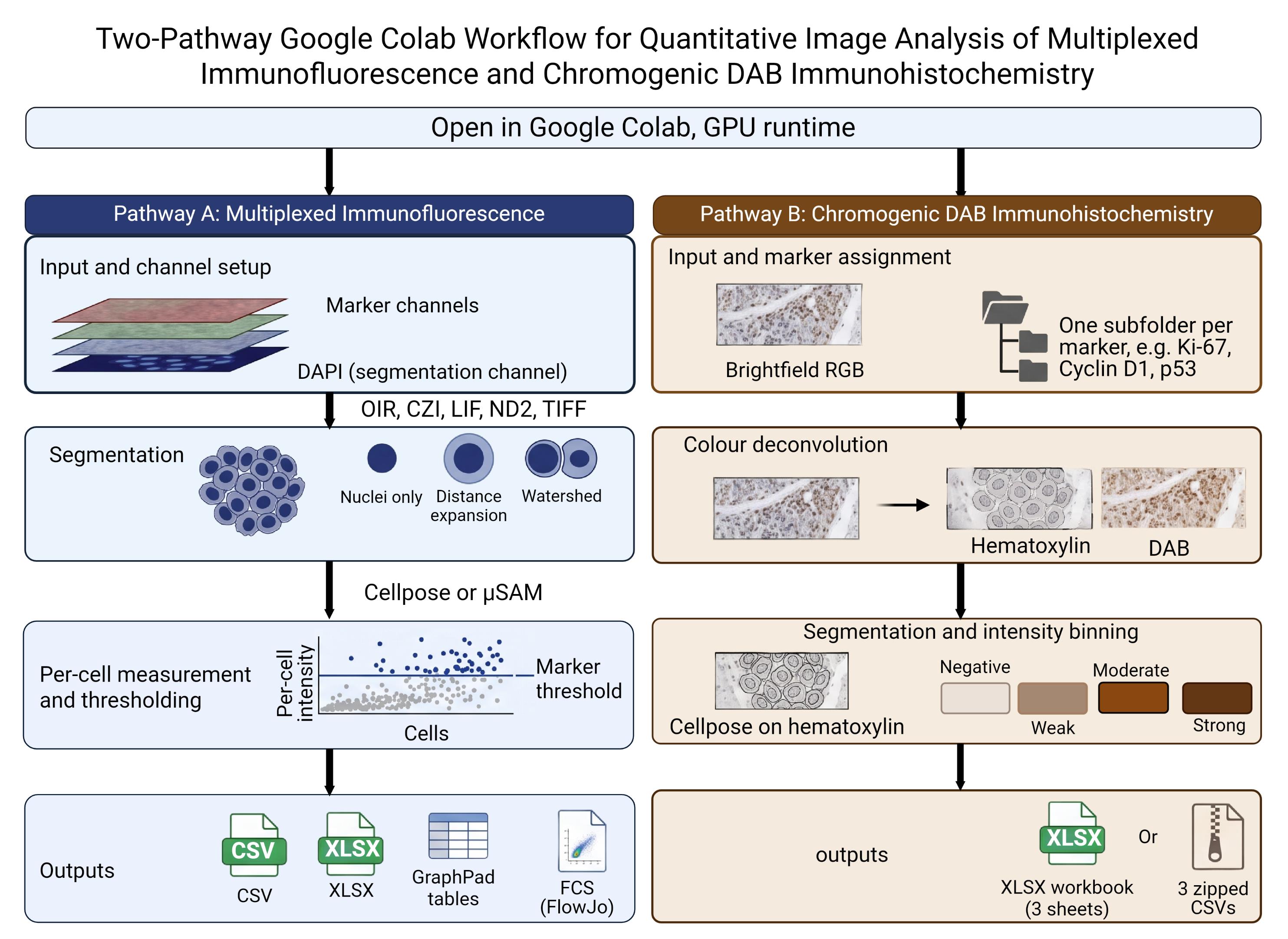
Quantitative analysis of multiplex immunofluorescence and chromogenic immunohistochemistry commonly requires specialized software, local installation, scripting experience, or substantial manual processing. Here, we describe a browser-based Google Colab workflow that enables researchers to perform cell segmentation, staining quantification, phenotypic classification, quality control, and data export through interactive controls without editing code or installing software locally.
The notebook provides separate branches for fluorescence and chromogenic analysis. The fluorescence branch supports multichannel images and z-stacks, segments nuclei using pretrained Cellpose models, constructs nuclear or expanded cell-measurement regions, and quantifies per-cell fluorescence intensity and morphology. Marker-positive, double-positive, and triple-positive populations can be classified using user-selected thresholds, and results can be exported as CSV, XLSX, or FCS 3.1 files. Technical concordance was evaluated using a publicly available 44-channel t-CyCIF tonsil image and its published single-cell measurements. DNA1 re-segmentation produced 61,173 objects, of which 17,614 were matched to published cells using predefined centroid-distance and area-ratio criteria. Continuous fluorescence agreement and independently thresholded positive-cell classifications were assessed across DNA1 and 26 biological-marker channels. The chromogenic branch was evaluated in two complementary settings. First, perinuclear measurements were compared with pathologist-assigned HER2 grades using a balanced set of 4,000 image patches. The workflow correctly reproduced the four HER2 grades in approximately seven out of ten patches, with stronger agreement for perinuclear measurements than for nuclear measurements. Second, the workflow was tested against Human Protein Atlas staining-intensity annotations across 1,709 cancer tissue cores, covering 22 antibodies and 20 cancer types. Agreement was above the level expected by chance and remained similar when thresholds were fitted on one subset of cores and evaluated on a separate subset of cores, indicating that the results were not driven solely by scoring the same samples used to set the thresholds. This workflow provides an accessible and reproducible starting point for quantitative fluorescence and chromogenic image analysis.
Key features
• Runs in a browser through Google Colab with GPU access; no local installation or code editing required.
• Fluorescence: reads OIR, CZI, LIF, ND2, TIFF, PNG, and JPEG; segments with Cellpose or micro-SAM; exports per-cell measurements as CSV, XLSX, or FCS 3.1.
• Chromogenic: H-DAB or custom color deconvolution; H-scores in nuclear, perinuclear-ring, or whole-cell compartments, or area-based scoring; thresholds anchored to negative controls.
• Evaluated against pathologist HER2 grades (4,000 patches) and Human Protein Atlas intensity annotations (1,709 cores, 22 antibodies, 20 cancers); thresholds fitted out of fold.
Keywords: Multiplex immunofluorescence Chromogenic immunohistochemistry
Image segmentation
Cellpose
Segment Anything for Microscopy
Google Colab
Color deconvolution
H-score
Stained area fraction
Negative control
HER2
Human Protein Atlas
Reproducible image analysis
Graphical overview
Background
Quantitative tissue-image analysis depends on reliable identification of individual objects and a transparent conversion of pixel values into cell-level measurements. Cellpose provides a generalist approach to cellular segmentation [1], and recent releases include pretrained Cellpose-SAM models [2]. The notebook uses the Cellpose models detected in the installed package and can also install Segment Anything for Microscopy (micro-SAM) as an alternative method for two-dimensional nuclear segmentation [3]. Because these models are pretrained, they can be applied without first assembling a training dataset or developing a new segmentation model. This browser-based approach avoids the local installation and scripting experience that conventional image-analysis software commonly requires.
Microscopy images are frequently stored in proprietary formats, with pixel data and acquisition metadata encoded differently by each manufacturer. To address this problem, the notebook uses BioIO [4] and supporting readers to open OIR, CZI, LIF, ND2, TIFF, PNG, and JPEG files and organize their pixel data in a common TCZYX representation. An AICSImageIO import fallback is retained for compatible environments. Bio-Formats is used specifically to support OIR reading and metadata access [5], while AICSImageIO is retained as a compatibility fallback when BioIO is unavailable. After import, users assign the nuclear and marker channels, select a Z-projection method, and inspect the resulting images before segmentation.
The fluorescence branch can retain the resulting labels as nuclear masks or expand them to approximate a larger cellular compartment. It then uses scikit-image [6] to process the masks and obtain per-object fluorescence intensity and morphological measurements. Marker-intensity distributions are displayed before thresholds are selected, allowing objects to be classified as positive or negative for individual markers and marker combinations.
The chromogenic branch relies on color deconvolution, which recovers each dye's contribution from an RGB image using its optical density vector [7]. For H-DAB images, the notebook performs color deconvolution using the Ruifrok and Johnston hematoxylin-eosin-DAB vectors implemented in scikit-image. Users analyzing other chromogens may instead provide custom stain vectors. Each supplied vector is normalized to unit length; if only two vectors are provided, the notebook calculates a third by taking their cross product. As quality-control measures, it reports the angle between each pair of vectors and the condition number of the resulting matrix. Vectors that are too similar produce unstable stain separation and can amplify small color differences between slides. Because stain appearance varies with laboratory procedures and scanner settings, published presets for stains such as trichrome or Alcian blue may not transfer reliably between laboratories. Custom vectors for such analysis should therefore be estimated from single-stain control slides prepared under the same conditions and imaged using the same scanner.
Two analysis modes are provided because chromogenic staining cannot always be assigned to individual cells. In cell-based mode, nuclei are segmented using the counterstain, and chromogen optical density is measured for each cell within the nuclear, perinuclear ring, or whole-cell compartment. Cells are classified as negative, weak, moderate, or strong, and the proportions in the three positive categories are used to calculate the H-score. In the area-based mode, which is intended for collagen and other extracellular or diffuse targets, cell segmentation is omitted. Instead, the proportion of tissue area within each intensity category is measured. The resulting area fractions and any weighted area-intensity score calculated from them are not H-scores because their denominator is tissue area rather than cell number.
Both modes use the same threshold-selection panel, although their thresholds are estimated separately because one uses mean optical density per cell and the other uses pixel-level optical density within tissue. When available, a matched technical negative control can be used to directly establish the negative/weak boundary. This should be a section processed alongside the samples, with the primary antibody omitted or replaced with an appropriate isotype control, while retaining the same detection system and chromogen steps. A tissue sample assumed to be biologically negative is not equivalent to this technical control. The control image is analyzed using the same stain profile, compartment, and processing settings as the corresponding samples. Its upper optical-density tail defines the amount of background permitted above the negative/weak threshold. This is the only automated threshold option that does not require the sample set itself to contain a distinct negative population; the weak/moderate and moderate/strong boundaries must still be estimated from the samples or adjusted manually.
Interactive widgets guide users through image import, channel assignment, segmentation, measurement, threshold selection, visualization, and export. The notebook supports both individual images and batch processing, retains intermediate images for inspection, and allows parameters to be adjusted before final export. It also records the selected segmentation method and measurement mask geometry. For immunofluorescence analysis, cell-level measurements can be exported in FCS format for use in compatible downstream software. This ready-to-use workflow makes advanced image analysis more accessible for routine research.
The notebook is designed primarily for Google Colab, a hosted Jupyter environment that may provide access to GPUs; however, accelerator type, memory, availability, and session duration are not guaranteed (if not familiar with Google Colab, read more here [8]). It can also be adapted for Kaggle (if not familiar with Kaggle, read more here [9]) or a local Jupyter environment, and CPU execution is still possible, though it may be slower. Ease of use does not remove the need for biological controls, standardized image acquisition, segmentation assessment, or appropriate statistical analysis. The fluorescence and chromogenic branches should therefore be evaluated independently for each imaging platform, tissue type, staining panel, and scientific question.
Materials and reagents
Laboratory supplies
No laboratory consumables are required for the computational procedure. Ensure that original images and associated metadata have been retained in read-only archival storage.
Equipment
1. Internet-connected computer with a current web browser
2. Google account with access to Google Colab and, for batch processing, sufficient Google Drive storage; we recommend GPU support (some GPU resources were free for limited use in Google Colab and in Kaggle while writing this protocol)
3. Local or network storage for original images and exported results
4. (Optional) Local CUDA-capable workstation if the notebook is adapted to a local Jupyter runtime; local execution is outside the validated scope of this protocol
Software and datasets
1. MultiplexIF_Analysis_Suite.ipynb (Github: https://github.com/arunviswanathan91/ImageAnalysis) (Zenodo: https://doi.org/10.5281/zenodo.22260636)
2. Google Colab
3. Python; the stored execution used Python 3.12.13
4. Cellpose; the stored execution reported Cellpose 4.2.1.1; model names are read from the installed package at runtime
5. PyTorch; the stored execution reported PyTorch 2.11.0+cu128
6. micro-sam/μSAM
7. BioIO, bioio-bioformats, and bffile, with Bio-Formats 8.1.1
8. NumPy, SciPy, and scikit-image; the stored execution reported NumPy 2.5.1, SciPy 1.18.0, and scikit-image 0.26.0
9. Supporting readers: aicspylibczi, readlif, nd2, tifffile, and Pillow
10. pandas, Matplotlib, seaborn, ipywidgets, openpyxl, tqdm, and psutil
11. Input data: Fluorescence or brightfield chromogenic images, including representative positive, negative, and technical control images appropriate to the experimental design.
Datasets
1. External Validation dataset 1, Fluorescence branch: TONSIL-1 t-CyCIF image [10]. Direct URL to data: https://www.synapse.org/Synapse:syn17865732/wiki/592782
2. External validation dataset 2, chromogenic branch: HER2-IHC-40x [15]. Direct URL to data: https://zenodo.org/records/15179608
3. External validation dataset 3, chromogenic branch: Human Protein Atlas cancer pathology images with per-patient IHC intensity annotation [16,18]. Direct URL to data: https://www.proteinatlas.org. Can be accessed through The Image Data Resource (IDR): https://idr.openmicroscopy.org/webclient/?show=project-501
Critical: Several packages are installed without exact version pins, although Bio-Formats is fixed at 8.1.1 in the current notebook. Preserve the notebook, installation output, version report, model name, runtime hardware, and analysis date with every result set. Before publication, archive a tested notebook (Table 1) release and an environment specification.
Table 1. Default analysis parameters as supplied in the notebook. These are starting values, not validated settings. Record the values used for every analysis. Steps are named as in this protocol.
| Step | Parameter | Default | Applies to |
| 3 | Z-projection | Maximum intensity | Fluorescence |
| 4 | Segmentation engine | Cellpose | Fluorescence |
| 4, H3 | Cellpose model | cpsam_v2 when present in the installed registry | Both branches |
| 4, H3 | Diameter (px) | 0, automatic estimation | Both branches |
| 4, H3 | Flow threshold | 0.40 | Both branches |
| 4, H3 | Cell probability threshold | 0.0 | Both branches |
| 4, H3 | Minimum mask size (px) | 15 | Both branches |
| 5A | Mask geometry | Distance-based expansion | Fluorescence |
| 5A | Expansion ratio | 0.50 | Fluorescence |
| 5A | Watershed cap ratio | 1.0 | Fluorescence |
| 6 | Threshold method | Otsu | Fluorescence |
| H1 | Stain profile | H-DAB, Ruifrok and Johnston vectors | Chromogenic |
| H1 | Negative controls | None registered | Chromogenic |
| H2 | Analysis mode | Cell based | Chromogenic |
| H2 | Measurement compartment | Nuclear | DAB Chromogenic, cell mode |
| H3 | Expansion ratio | 0.50, set separately for each expanding marker | Chromogenic, ring and whole cell |
| H3 | Tissue mask offset | 1.00, the Otsu value itself | Chromogenic, area mode |
| H3 | Smoothing sigma (px) | 3.0 | Chromogenic, area mode |
| H3 | Tiling | Off; 512 px tiles and a minimum tissue fraction of 0.10 when enabled | Chromogenic, area mode |
| H4 | Threshold scope | Per marker | Chromogenic |
| H4 | Threshold method | Otsu on log10 optical density, then fixed log offsets1 | Chromogenic |
| H4 | Upper log10 offsets | 0.398 and 0.699 above the negative cut1 | Chromogenic |
| H4 | Control tolerance | 0.01 for cell mode; 0.001 is the usual value for area mode | Chromogenic |
| H4 | Intensity bands | Three: weak, moderate and strong | Chromogenic |
| 4, 7, 10, H3 | Figure export resolution | 150 dpi | Both branches |
Note: Every threshold in step H4 is proposed automatically and remains independently adjustable before scoring. The stored value is whatever the slider reads when the thresholds are applied, and the export records whether a slider was moved after the automatic estimate.
1A reporting convention chosen during exploratory analysis, not derived from a physical, biological, or calibration-based model; see step H4 for discussion.
Procedure
Before beginning this procedure: Lettered sections (A, B, C...) and their numbered sub-steps give the sequence to follow in this protocol; mentions of Step N (in italics) refer to the Google Colab notebook’s own internal cell labels, a separate system that does not always match this sequence (see General note 13). For the purposes of this protocol, we will use the default values listed in Table 1.
A. Prepare image files and metadata
1. Copy the original image files (raw files) to a read-only archive. Perform analysis on a working copy.
2. For fluorescence analysis, use one of the supported extensions: .oir, .czi, .lif, .nd2, .tif, .tiff, .png, .jpg, or .jpeg.
3. For chromogenic immunohistochemistry analysis, use an RGB .tif, .tiff, .png, .jpg, or .jpeg file. One stain profile applies to a whole run, so images stained with different chromogens are analyzed as separate runs.
4. Confirm that fluorescence images contain a nuclear channel. A pan-cellular or whole-cell counterstain is optional but is required for signal-guided watershed expansion.
5. (Optional) Organize batch fluorescence images so that folder names correspond to meaningful samples or experimental conditions. The notebook can apply one channel map to all files, one map per folder, or one map per file.
6. For batch chromogenic analysis, place images in a master folder with one subfolder per marker. The subfolder name is proposed as the marker label and can be edited for each file. Keep the negative control images for that staining run in a separate subfolder of the same master folder, so that the control travels with the batch it calibrates and can be registered directly in step H1. An option to upload the control images is available; however, we advise uploading them to Google Drive for ease of access.
7. Prepare an analysis record containing the study identifier, staining panel, acquisition instrument, objective, pixel size, bit depth, biological replicate, technical replicate, and control status.
Critical: Do not compare raw fluorescence intensity across images acquired with different exposure, laser power, detector gain, bit depth, or other acquisition settings unless an experimentally justified normalization or calibration strategy has been applied outside the notebook.
B. Start the Colab runtime and configure the environment
1. Open the notebook in Google Colab. Figure 1 shows the flowchart of the entire fluorescence workflow.
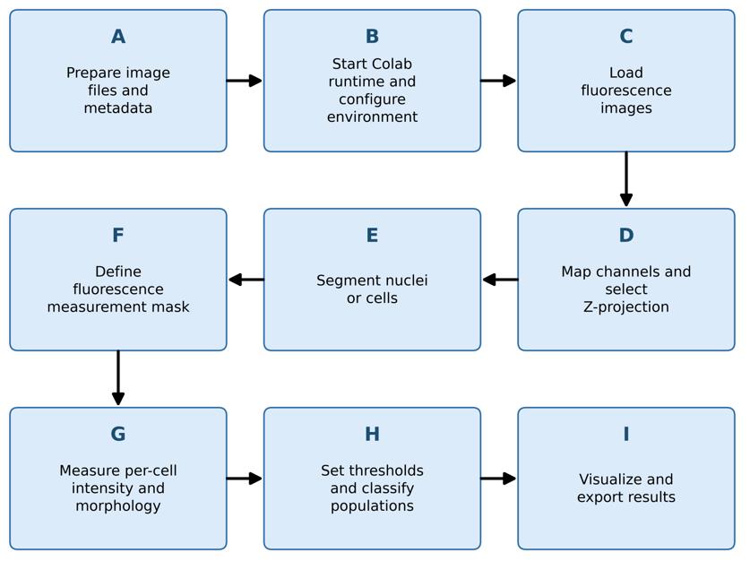
Figure 1. Fluorescence branch workflow. Sequence of sections A–I in the Procedure for fluorescence image analysis, from image preparation (A) through visualization and export (I). Labels correspond to the lettered sections described in the text.
2. Select Runtime → Change runtime type and request a GPU hardware accelerator when available.
3. Run Step 1 - Environment Setup & GPU Check once.
4. Retain the complete installation output. Confirm that the notebook prints the status of Python, PyTorch, GPU, RAM, NumPy, SciPy, scikit-image, tifffile, Cellpose, BioIO, and Java.
5. Allow the cell to restart the kernel. Colab may display a session crash message because the notebook intentionally restarts the kernel after installing packages.
6. Continue directly to Step 2 (Procedure, step C1) after reconnection. Do not rerun Step 1 in the same runtime unless the environment has been reset.
Critical: Before processing study data, review the version report generated by the setup cell and test at least one representative file of each format to be analyzed. The notebook installs the BioIO reader stack without pinning tifffile, then reinstalls NumPy, SciPy, and scikit-image before restarting the runtime. Bio-Formats is pinned to version 8.1.1 and loaded from a JAR downloaded to the Colab runtime when possible, with Maven resolution used as a fallback. Because most Python packages are not pinned to exact versions, the resolved environment may change between Colab sessions. Retain the version report with the analysis records and repeat the compatibility tests after package or runtime updates.
Note: All fluorescence images used in the protocol demonstration were acquired with an Olympus FV3000 and are stored with the .oir extension. The notebook was executed on an NVIDIA Tesla T4 with High RAM for image analysis. Whole-slide stitched images of mIF slides were analyzed using an A100 with high RAM.
C. Load fluorescence images
1. Run Step 2 - File Upload & Format Detection.
2. Select one input mode:
a. Upload file for one local file;
b. Google Drive - single file for one file stored in Drive; or
c. Google Drive - folder (batch) for multiple files.
3. For a batch folder, choose whether the scan is recursive (to include subfolders), review the detected files, deselect unwanted files, and confirm the selection.
4. Load the first selected file and confirm the reported TCZYX dimensions, channel names, bit depth, physical pixel size, objective metadata, filename, and sample label. Step 2 also displays individual-channel and composite previews (Figure 2). Preview LUT colors are assigned for visualization and do not define biological channel identities. A transmitted-light channel, when present, may therefore appear in an arbitrary display color until channel roles are assigned in Step 3.
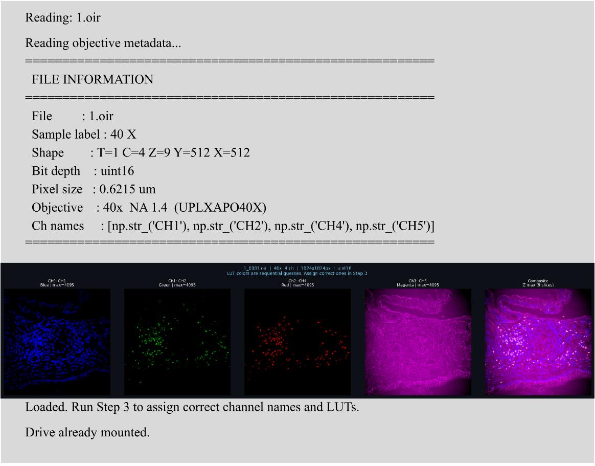
Figure 2. Image-import output from Step 2. The panel reports file and acquisition metadata and displays individual channels with a composite preview. Automatically assigned LUT colors are for visualization only.
5. Record missing or implausible metadata in the analysis record. Do not infer a physical pixel size from magnification alone.
Notes:
1. The notebook uses the first time point (T = 0) for subsequent fluorescence analysis. Time-series analysis is not implemented in this version.
2. LIF loading is limited to the first image and explicitly reads the first Z, time, and mosaic frames. TIFF axis interpretation is partly heuristic: a three-dimensional array with a first dimension of eight or fewer is treated as channel-first; otherwise, it is treated as a Z-stack. Confirm axes independently for representative LIF and TIFF inputs.
D. Map fluorescence channels and select a Z-projection
1. Run Step 3 - Channel Mapper.
2. Inspect the per-channel thumbnails and the composite display. Display thumbnails are downsampled, but analysis uses full-resolution arrays.
3. Assign exactly one included channel to Nuclei/DAPI (Figure 3). Assign a Pan-cellular marker only when the channel reports a suitable whole-cell boundary signal. Assign all remaining included channels’ biological marker names.
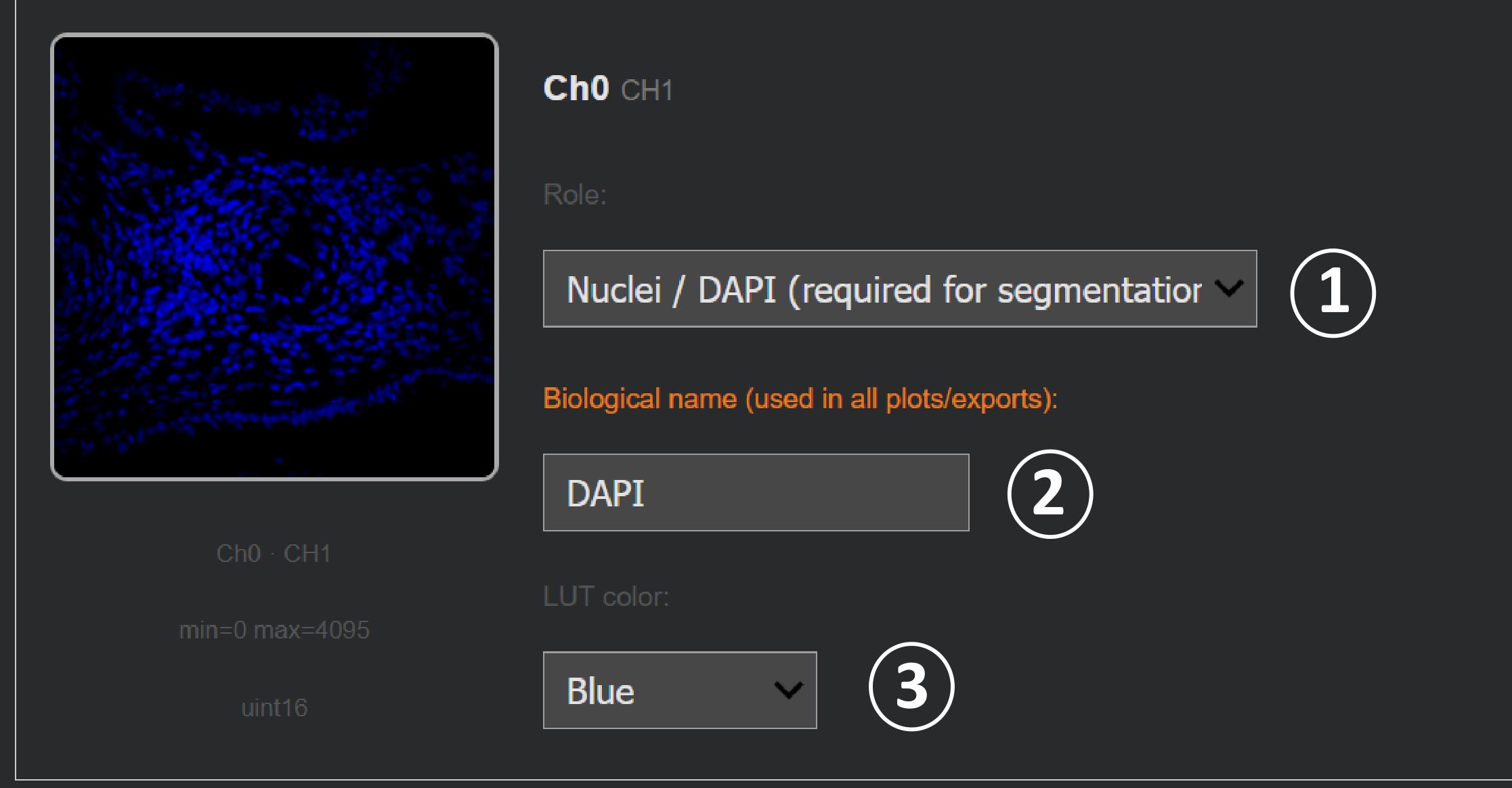
Figure 3. Channel assignment in Step 3. The channel mapper is used to (1) select an analytical role, (2) enter the biological channel name, and (3) choose a display color. The example assigns the displayed channel to Nuclei/DAPI and names it DAPI.
4. Exclude channels that should not contribute to analysis.
5. Use each analytical role only once. The current interface provides 12 generic marker roles; assigning the same role to multiple channels overwrites the earlier role entry.
6. Select one Z-projection:
a. Max Intensity (default),
b. Mean Intensity, or
c. Sum (optical sections).
7. Confirm the channel setup.
8. For batches, specify whether assignments are shared by all files, shared within folders, or defined per file. Review every group before confirming.
Critical: The selected projection is applied before segmentation and intensity measurement. Use the same projection rule for the images to be compared.
Note: The Step 2 and Step 3 previews are always rendered as maximum projections, irrespective of the projection selected here. Only the analysis path applies the chosen Mean or Sum rule, so a preview image can differ from the measured array.
E. Segment nuclei or cells
1. Run Step 4 - Cellpose Segmentation (Interactive).
2. Review the detected Cellpose version, available model names, GPU status, nuclear-channel name, pan-cellular assignment, and image dimensions.
3. Select the segmentation engine (see Table 2 and Table 3 before deciding which model to select):
a. Cellpose (default) or
b. μSAM. The μSAM option is always displayed and is relabeled (not installed) when the import fails, so confirm from the printed availability line, not from the presence of the option, that μSAM is usable before selecting it.
Table 2. Cellpose models offered for nuclear segmentation in both branches and suggested use.
| Name | Backbone | Suggested use |
|---|---|---|
| cpsam_v2 | SAM-ViTL | Cellpose-SAM model with a training correction for low-contrast regions; a reasonable starting point when it is present in the installed registry. |
| cpdino | DINOv3-ViTL | Uses a 384 × 384 processing tile to provide greater spatial context. Consider it for large, elongated, or densely packed objects when the SAM-based model merges or fragments them. |
| cpdino-vitb | DINOv3-ViTB | Smaller and faster DINOv3 variant that may be useful for large batches or limited GPU memory. |
| cpsam | SAM-ViTL | Original Cellpose-SAM release. Use when reproducing an analysis performed with this model; the first use may require an approximately 1.1 GB download. |
Table 3. micro-SAM models offered as an alternative segmentation engine in the fluorescence branch. micro-SAM is not offered in the chromogenic branch, which segments with Cellpose only.
| Name | Suggested use |
|---|---|
| vit_b_lm | Light-microscopy generalist and the notebook default; smaller and faster than vit_l_lm. |
| vit_l_lm | Larger light-microscopy generalist that requires more time and memory; evaluate when the smaller model does not provide acceptable masks. |
| vit_b | Generic Segment Anything base model rather than a microscopy-specific model; use only as an alternative when the light-microscopy variants are unsuitable. |
4. For Cellpose, select an available model from the runtime-generated list.
5. If Cellpose version 4 or later is available and a suitable pan-cellular channel was assigned, decide whether to enable dual-stain whole-cell segmentation. Otherwise, retain DAPI-only segmentation.
6. Start with the notebook defaults for Cellpose (Table 1):
a. Diameter = 0 pixels (automatic estimation),
b. Flow threshold = 0.40,
c. Cell probability threshold = 0.0, and
d. Minimum size = 15 pixels squared.
7. (Optional) Run segmentation on one representative file before starting a batch.
8. Inspect the original image, segmentation overlay, boundaries, cell count, and apparent errors. Evaluate under-segmentation, over-segmentation, merged nuclei, fragmented masks, missed dim nuclei, and background objects. Figure 4 shows an example of the output after segmentation using the nuclear mask alone.
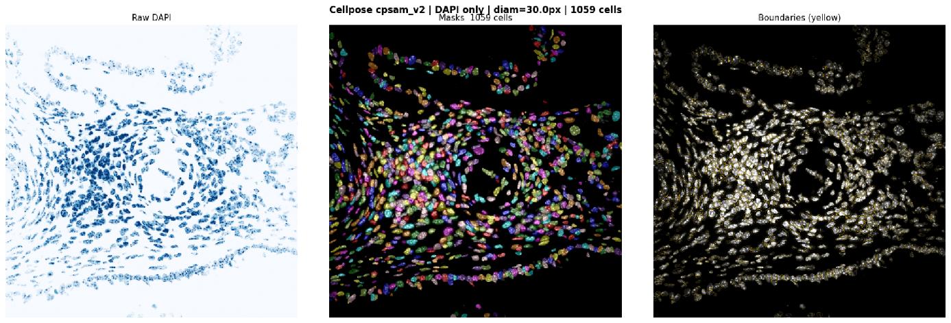
Figure 4. Cellpose segmentation output. The exported panel shows the projected DAPI image (left), the labeled-mask overlay (middle), and object boundaries (right). The figure shows the selected model and the number of detected objects, and it can be saved for each image.
9. Adjust one parameter at a time and rerun the representative file until the masks are acceptable for the intended analysis.
10. Process the batch only after selecting fixed parameters. Save the segmentation figures and record the parameter values.
Critical: Visual acceptability on one image is not evidence of accuracy across a dataset. Review representative images from every tissue type, staining batch, acquisition settings, and experimental group.
Limitation: The fluorescence workflow relies primarily on the nuclear channel for segmentation. micro-SAM uses DAPI alone in this implementation, whereas compatible Cellpose models can additionally use an assigned pan-cellular channel for whole-cell segmentation. Nuclear masks may underestimate cytoplasmic or membrane-associated signals. Distance-based or marker-guided expansion can reduce this loss but may also include background or signal from neighboring cells; neither approach is universally preferable, and the selected geometry should be evaluated for each marker and tissue. In exploratory 40× images, classifications for CD4, CD8, TIM-3, and granzyme B changed little between nuclear and expanded masks, but this comparison was not systematically assessed in the present protocol and should not be generalized. We suspect this might be due to the small cell sizes at 40×, which resulted in low-resolution fluorescent markers of these small immune cells. At higher magnification, when resolution is high, these decisions might affect the analysis greatly.
F. Define the fluorescence measurement mask
1. Run Step 5A - Mask Expansion after segmentation.
2. Select one mask geometry:
a. Nucleus only to use the raw segmentation labels,
b. Distance-based expansion to expand each label without overlap, or
c. Watershed when a pan-cellular channel is available.
3. For distance-based expansion, begin with the default expansion ratio of 0.50. The expansion radius is calculated as:
Where dnuclear is the estimated nuclear diameter in pixels, and α is the user-selected expansion ratio. The lower bound ensures that distance expansion adds at least one pixel. The value Rexp is the width added around the nuclear mask, not the final cell radius. For example, when dnuclear = 20 pixels and α = 0.50, the mask expands outward by 5 pixels.
If no diameter is returned by the segmentation model, the code will estimate the diameter from the nuclear mask as:
Where Ai is the area of the nucleus in pixels. If no labeled objects are available, the code uses 30 pixels as a last-resort default. Figure 5 shows the output of segmentation with the nuclear mask and the expanded nuclear mask using the formula discussed above.
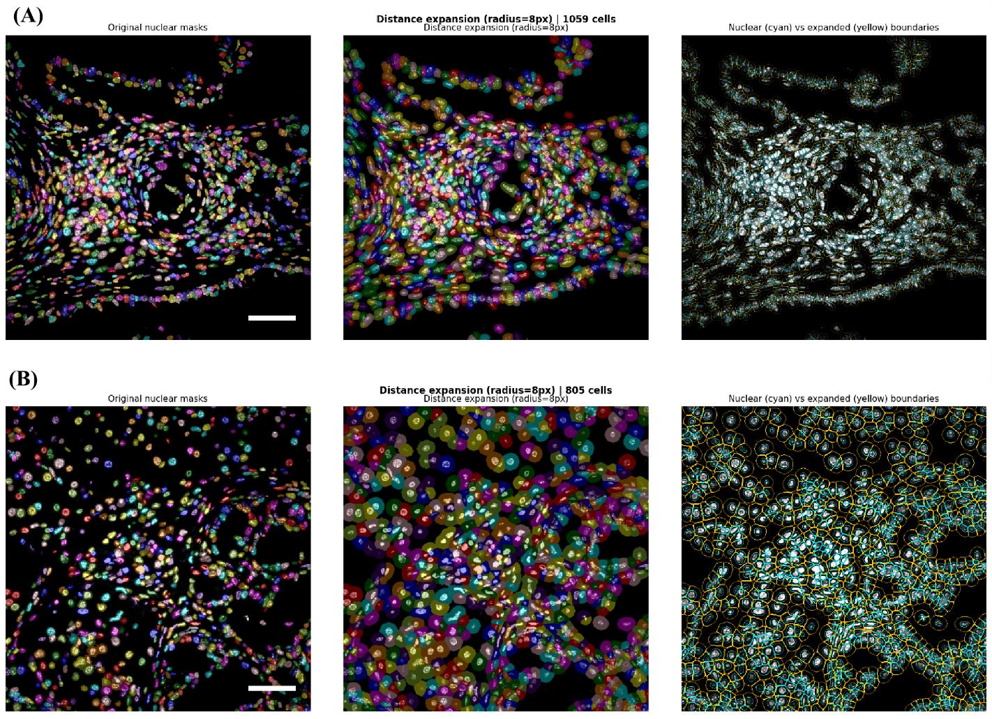
Figure 5. Examples of fluorescence measurement-mask expansion. Panels A (40×) and B (60×) compare nuclear boundaries (left) with the corresponding expanded masks (middle) and their respective segmented boundaries (right) in two input images at different magnifications. Note that an 8px increase results in a different expanded area at both magnifications (the middle of both panels). Scale bars = 20 μm.
4. For watershed expansion, begin with the default cap ratio of 1.0. The notebook normalizes the pan-cellular channel for boundary detection, computes a Sobel elevation map, expands labels via watershed, and limits growth to a distance-based cap.
5. Inspect the expanded boundaries. Confirm that adjacent cells do not overlap and that expanded masks do not capture large background regions.
6. Apply the chosen geometry to the single image or batch.
7. Record the mask method, expansion ratio, or cap ratio, calculated pixel radius, and whether any file required fallback behavior.
Critical: The selected geometry is applied uniformly to all measured marker channels. Per-marker compartment masks are not implemented. If a panel contains both nuclear and membrane/cytoplasmic markers, quantify the consequences of this simplification before interpreting population frequencies.
G. Measure per-cell fluorescence and morphology
1. Run Step 5 - Per-Cell Intensity Measurement.
2. Confirm that the displayed segmentation engine and mask source match the preceding steps.
3. Allow the notebook to calculate, for each labeled object:
a. Label identifier, area, and centroid (x_px, y_px),
b. Native mean, maximum, and minimum intensity for every included channel,
c. Major-axis length, minor-axis length, perimeter, eccentricity, and solidity,
d. Elongation, defined as minor-axis length divided by major-axis length,
e. Circularity, defined as 4π × area/perimeter2, and
f. Area in square micrometers when physical pixel size is available.
4. Review the first rows of the per-cell table. Confirm that expected marker columns are present and that intensities remain in the native image scale.
5. Export the intermediate per-cell CSV files if required. For batches, retain both per-file CSVs and batch_all_cells.csv.
Note: Display normalization does not change the intensity values used for per-cell measurement.
H. Set fluorescence thresholds and classify populations
1. Run Step 6 - Interactive Threshold & Cell Classification.
2. Inspect the raw mean-fluorescence-intensity distribution for each marker.
3. Review the automatic suggestions based on Otsu [11], Triangle [12], and Yen [13] thresholding. The default selection is Otsu (Figure 6). Otsu assumes two roughly separated populations, minimizes within-class variance, and performs best when positive and negative cells form two clear peaks. Triangle is suited to a skewed histogram with one dominant peak and a small, sparse positive tail. Yen tracks Otsu closely on clean bimodal data but can diverge when the populations are noisy or unevenly sized. Compare the shape of the marker’s histogram against these descriptions before accepting the default.
4. Select Manual when control samples, expert review, or a prespecified analysis plan support a different threshold.
5. For batches, select one threshold mode:
a. A global threshold set for all files,
b. A separate threshold set for each file, or
c. A threshold set shared within an experimental folder/group.
6. Apply thresholds. A cell is classified as positive when its marker mean intensity is greater than the selected threshold.
7. Review the total number and percentage of positive cells for each marker and for generated marker combinations.
8. Save every threshold value and threshold mode with the analysis record.
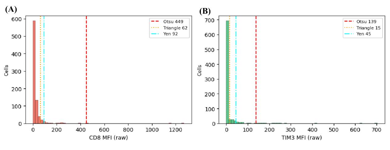
Figure 6. Fluorescence threshold selection in Step 6. Mean-fluorescence intensity (MFI) histograms for CD8 (A) and TIM3) (B) are shown with the Otsu, Triangle, and Yen threshold estimates.
Critical: Automatic histogram thresholds are suggestions, not biological ground truth. Define thresholds with appropriate negative, single-positive, and technical controls. Do not select a threshold solely because it yields an expected biological result.
Why threshold selection matters: In fluorescence analysis, the selected threshold determines which segmented cells are classified as marker-positive, thereby directly affecting the reported numbers and percentages of single-, double-, and multiple-marker-positive populations. Review automatic thresholds against appropriate controls and apply the selected values consistently across comparable images.
Critical: The current classification code treats every assigned role other than Nuclei/DAPI as a thresholded marker. A channel assigned as a Pan-cellular marker is therefore also classified unless it is excluded from downstream interpretation.
I. Visualize and export fluorescence results
1. Run Step 7 - Visualization Dashboard.
2. (Optional) Select the condition/group labeling rule and verify the mapping from filenames or folders to biological groups. When the immediate parent folder is a bare magnification label matching the pattern <digits>
3. Select the mask geometry to visualize. Keep this selection consistent with the geometry used for measurement.
4. Generate and inspect spatial population maps, marker scatterplots, population summaries, and bar charts (Figure 7).
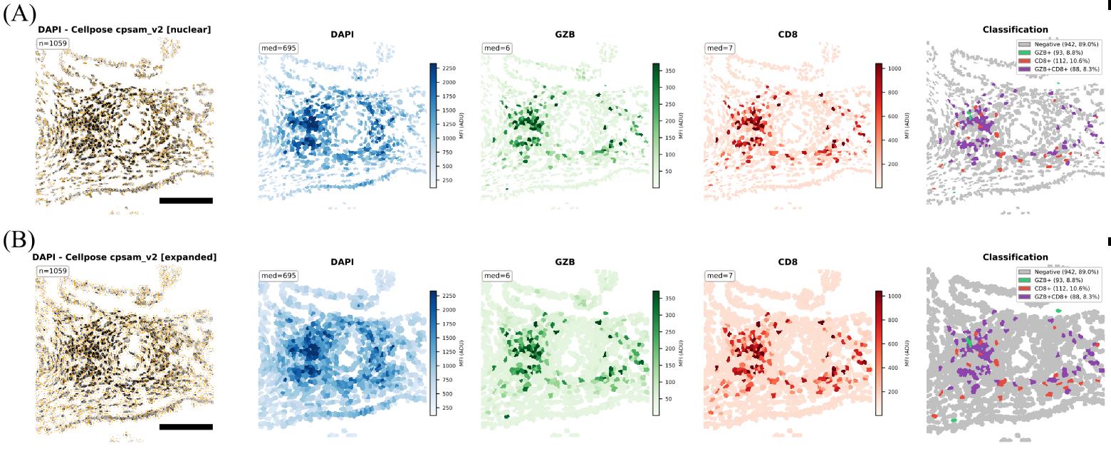
Figure 7. Fluorescence visualization output for DAPI, granzyme B (GZB), and CD8. The panels show (A) classification with nuclear masks and (B) classification with expanded masks. Scale bars = 100 μm.
5. Run Step 8 - Export - CSV/Excel/FCS.
6. Select the required columns and group labels. Export CSV and XLSX files.
7. If FCS export is required, select marker channels, spatial coordinates, morphology variables, and positivity flags. (Optional) Channels can be assigned fluorochrome names or excluded; the output can be written as one file per image or as a combined file; and the group label is encoded as a numeric Group-ID parameter for gating. The segmentation engine and mask geometry are written as FCS keywords unconditionally, independently of column selections.
Critical: FCS-based analysis is often useful for whole-slide scanning. However, a single-stained control image of each fluorochrome in the mIF is necessary for such analysis, as the FCS generated from it will be used downstream.
8. Run Step 8B - Graphing Export CSV when tables formatted for GraphPad Prism, R, or Python are required. This export writes a provenance text file alongside the tables and adds segmentation_engine and mask_geometry columns to the master per-cell CSV. Retain the provenance file with the results; it is the record of engine, mask geometry, and export settings for the methods description.
9. Run Step 10 - Shape & Morphology Analysis when distributions of area, circularity, elongation, eccentricity, solidity, axis lengths, or perimeter are required.
10. Save all outputs to a versioned result directory containing the notebook, version log, parameter record, thresholds, segmentation figures, exported data, and a copy of the original analysis plan. Steps 5, 7, and 8 can write directly to Google Drive and mirror the source folder structure, which is preferable to browser downloads for batches because the folder tags that identify each sample are preserved in the output paths.
Note: The notebook defaults to 150 dpi for several figure panels.
J. Analyze chromogenic immunohistochemistry images
1. Start Part 2 - Chromogenic Scoring Module. This branch is independent of the fluorescence workflow and shares only the segmentation models. Nothing carried over from Steps 2–10 is used here. Figure 8 shows the flow of the chromogenic module. Before starting the chromogenic scoring, see Table 4 to understand each step and how it will contribute to scoring.
Note: Installation of packages is common for both.
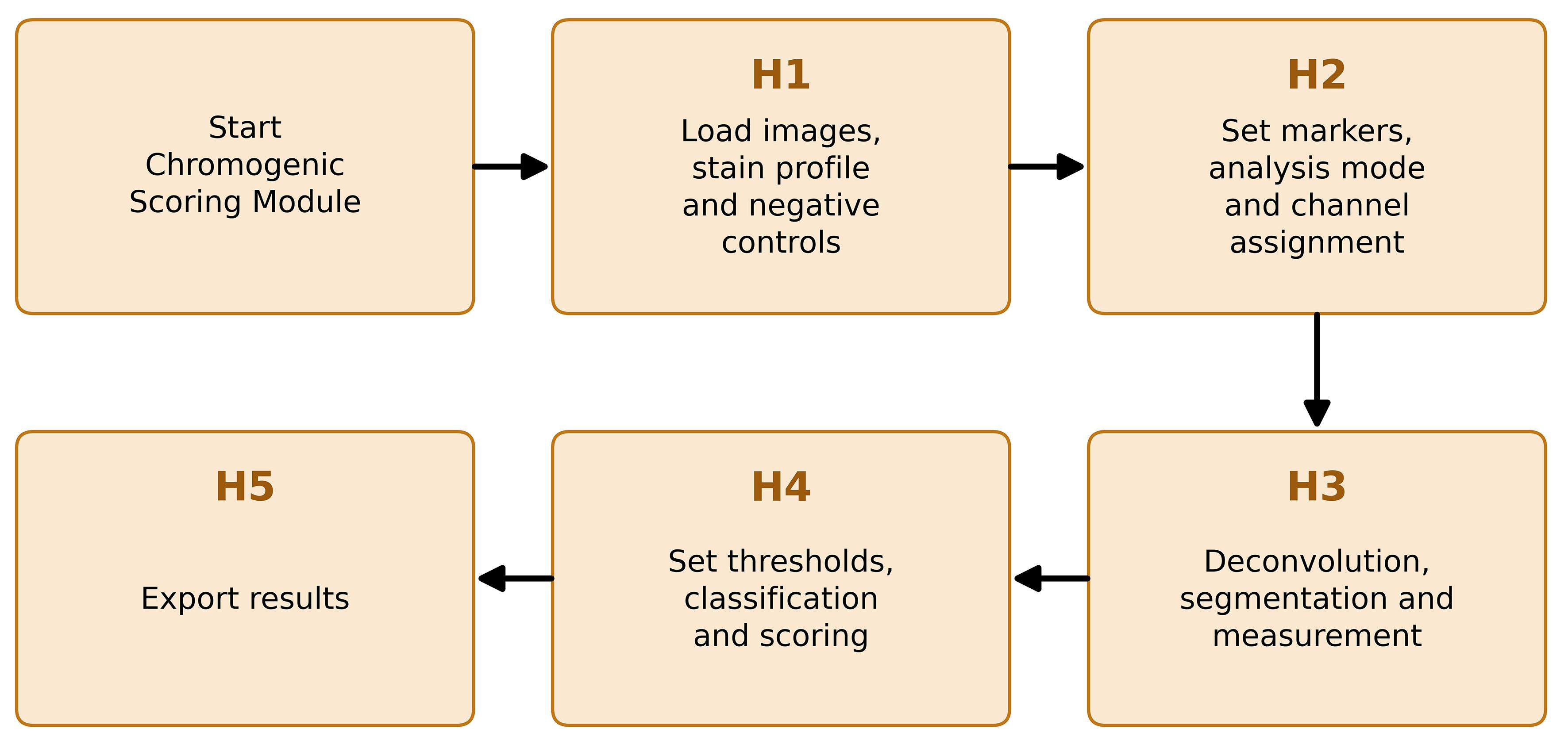
Figure 8. Chromogenic branch workflow. Sequence of steps within Procedure section J, following the notebook’s own internal labels (H1–H5), from loading images and registering the stain profile and negative controls (H1) through export of results (H5).
Table 4. Interactive controls, what each one changes, and how to judge the setting. A control listed against two steps behaves the same way in both branches. The segmentation models themselves are described in Tables 2 and 3.
| Control | Step | What it changes | How to judge the setting |
|---|---|---|---|
| Diameter | 4, H3 | Expected nuclear diameter given to Cellpose. Zero lets the model estimate it for every image. | Leave at zero unless the model consistently mis-sizes nuclei. A fixed value stops the estimate adapting between images of different magnifications. |
| Flow threshold | 4, H3 | How far a predicted mask may depart from the model's flow field before it is rejected. | Raise it when real nuclei are being dropped. Lower it when ragged or spurious masks appear. |
| Cell probability threshold | 4, H3 | The probability above which a pixel is taken to lie inside a cell. | Lower it to recover dim nuclei, raise it to suppress background objects. It changes mask extent as well as mask count. |
| Minimum mask size | 4, H3 | Smallest object retained, in pixels. | Raise it to remove debris and fragments. Set it against the true nuclear area at the magnification used rather than by eye on the overlay. |
| Expansion ratio | 5A, H3 | Width of the region added around each nucleus, as a multiple of half the nuclear diameter measured in that image. | At 0.50, the ring is about half a nuclear radius wide. Increase it only while adjacent cells remain separated and the ring stays on the tissue. |
| Watershed cap ratio | 5A | Maximum distance a label may grow under signal-guided watershed expansion. | Reduce it when expanded masks leak into background or into neighboring cells. |
| Tissue mask offset | H3 | Multiplies the Otsu threshold that separates tissue from glass in area mode. | 1.00 is the Otsu value itself. Below 1 admits fainter tissue; above 1 is stricter. This mask is the denominator of every area fraction, so check it on the preview. |
| Smoothing sigma | H3 | Gaussian smoothing applied to the chromogen channel before classification only. | Increase it when the classified mask is speckled. Mean optical density is measured on the unsmoothed channel and does not change. |
| Tile size and minimum tissue per tile | H3 | Size of the non-overlapping tiles and the tissue fraction a tile must hold to be kept. | Use tiles large enough to contain the structure of interest. Raise the minimum to discard edge tiles that are mostly glass. |
| Control tolerance | H4 | Fraction of negative control measurements allowed to fall above the negative cut. | 0.01 for per-cell measurements. Per-pixel populations have heavier tails, so 0.001 is the usual value in area mode. |
| The three intensity cuts | H4 | The negative, weak, and moderate boundaries, in raw optical density. | These override whatever the automatic method proposed and are what gets exported. Judge them on the classified image and on the negative control, not on the histogram alone. |
| Threshold method | 6 | Otsu, Triangle, or Yen estimate of the marker-positivity threshold in the fluorescence branch. | Read the estimate against negative and single-positive controls. Do not select a method because it returns the expected biological result. |
2. Run Step H1 - Load images, stain profile, and negative controls.
a. Select the stain profile. One profile applies to the whole run, because it fixes the deconvolution matrix and determines which options are offered downstream. H-DAB is the default profile used to evaluate the segmentation and scoring reported in this protocol. It is the correct choice for any brown DAB chromogen with a hematoxylin counterstain.
b. Select Custom stain vectors only for a chromogen other than DAB. Enter one optical density vector per stain, one stain per row. Two rows are sufficient; leaving the third at zero generates it by cross product. Press Validate matrix and read the reported condition number, determinant, inversion residual, and the angle between each pair of stain vectors.
c. Choose the image source. The upload file accepts one or more local files, all of which are placed in a single folder and therefore read as a single marker. In Google Drive, a single file takes one path. Google Drive: a master folder scans for subfolders, each holding the images for one marker; those subfolder names become the default marker tags in Step H2.
d. Inspect the preview of the first image, which shows the original alongside the three separated channels. Each channel should isolate the stain it names. A strong signal appearing in more than one channel indicates that the stain vectors do not match this staining.
e. Register negative control images when they are available. Give each control a short key name, such as no_primary or isotype_batch2, and mark it as run-wide when a single control slide covers the entire run. Markers claim these keys in Step H2, so one control image can serve one marker, several markers, or all of them.
f. Press Confirm run setup and check the printed summary before continuing. It lists the stain profile and its condition number, the number of sample images per folder, and each control key with the number of images associated with it.
Critical: A condition number above 20 or an angle below 15° between two stain vectors is reported as a warning rather than an error, and the run is allowed to proceed. A poorly conditioned matrix does not fail visibly; it converts small color differences between slides into large differences in the separated channels, so scores drift with staining batch rather than with biology. Do not use a custom profile that raises either warning without first re-deriving the vectors from single-stain control slides imaged on the same scanner. The matrix and its diagnostics are written to the Run_Metadata sheet at export and should be reported with the results.
Note on the role of negative controls: A negative control is a slide carrying no target signal, usually a no-primary or isotype control, processed in the same staining run and imaged on the same scanner at the same settings. With the primary antibody omitted, what remains is secondary antibody binding and chromogen deposition unrelated to the target. That is precisely the signal the negative threshold has to sit above. Without a control, the negative boundary is inferred from the samples themselves, which assumes that a negative population is present and separable in every batch. That assumption fails in a strongly stained tissue.
Note: The same control image is measured once for each marker that claims it, using that marker's compartment and settings, because background inside a nucleus and background in a perinuclear ring are different quantities. Control measurements are tagged and are excluded from every sample summary; they are used only to place thresholds and to report the false-positive rate those thresholds imply. A control from a different staining batch or scanner calibrates nothing, and supplying a mismatched control is worse than supplying none.
Note: Keep control images in Google Drive rather than uploading them through the browser. The upload channel reports no progress and is unreliable above roughly 50 MB per file, whereas reading from a Drive folder is disk-read-only. A workable arrangement is one Drive master folder per staining run, holding one subfolder per marker and a single control subfolder beside them, so that the control travels with the batch it belongs to and can be pointed at directly in Step H1. Retaining the controls in Drive also means the same threshold can be reproduced in a later session by importing the exported thresholds file.
3. Run Step H2 - Markers, analysis mode and channel assignment. Each subfolder appears as one row. Edit the marker name when the folder name is not the name to report; names must be unique, since two folders sharing a name would be pooled under a single threshold.
a. Set the analysis mode for each marker. Cell-based segments nuclei on the counterstain and returns an H-score from per-cell optical density. Area-based measures the stained fraction of tissue, performs no segmentation, and is the correct choice for targets with no cellular denominator, such as collagen, fibronectin, laminin, and other matrix proteins, where an H-score has no meaning.
b. Set the measurement compartment for each cell-based marker. Nuclear measures inside the segmented nucleus include Ki-67, p53, PCNA, pSTAT3, ER, and PR. The perinuclear ring expands the nuclear label and subtracts the nucleus, leaving a ring, and suits HER2, EGFR, PD-L1, and E-cadherin. Whole-cell measures inside the expanded label, including the nucleus, and suits cytoplasmic targets.
c. Confirm the target channel. For H-DAB, this is fixed at channel 2 (the DAB channel), and the counterstain is fixed at channel 0. For a custom profile, both are chosen here, in the order the vectors were entered.
d. Assign a control key to each marker where controls were registered in Step H1. A key marked run wide is preselected for every marker and can be changed row by row, and the bulk selector sets one key for the whole table. A marker left on none has its threshold estimated from the samples in Step H4; this is the default behavior, not an error.
e. Enable the per-file override table when a single subfolder holds images stained for different markers and assign the marker for each file individually.
f. Press Confirm marker assignment and read the printed table. It reports the mode, compartment, target channel, and control key for every marker, how many control measurements will run in Step H3, and which markers have no control assigned.
Note: A perinuclear ring approximates the membrane compartment from nuclear geometry. It is not a segmented membrane boundary. A nuclear mask applied to a membranous marker measures the unstained cell interior and under-reads the signal, which is the failure the ring is there to avoid; the ring, in turn, includes whatever lies immediately outside the nucleus, including a signal from a neighboring cell where cells are tightly packed. This perinuclear ring can be used if the DAB shows puncta in the images or in case of membrane-rich expression.
4. Run Step H3 - Deconvolution, segmentation, and measurement. Set the parameters, preview one representative image for each marker, then process the batch.
a. Select a Cellpose model (Table 2) and begin with the notebook defaults: diameter 0 for automatic estimation, flow threshold 0.40, cell probability threshold 0.0, and minimum mask size 15 pixels.
b. Set the expansion ratio separately for each expanding marker (Figure 9C, E). Nuclear markers (Figure 9B) are measured on the unexpanded mask and take no ratio as input. Beginning from the default of 0.50, the expansion distance in pixels is
where α is the expansion ratio, and
taken over the segmented nuclei of area A. The radius is therefore recalculated for each image and scales with magnification rather than being a fixed pixel count. Label expansion is collision-aware, so neighboring objects do not overlap. The same ratio is applied to any negative control claimed by that marker.
c. For area-based markers (Figure 9D), set the tissue mask offset and the smoothing sigma. Tissue is separated from glass by Otsu thresholding of the total optical density of the RGB image,
summed over the three channels of intensity I. A pixel is assigned to tissue when its total optical density is at or above k times the Otsu value, where k is the tissue mask offset. At the default of 1.00, the offset is the Otsu value itself; below 1, fainter tissue is admitted; above 1, the mask is stricter.
Critical: This mask is the denominator of every area fraction, so check it on the preview before running.
d. Enable tiling for large, stitched scans or where a heterogeneity map is wanted. Non-overlapping tiles are measured separately, tiles below the minimum tissue fraction are discarded as glass or artifact, and thresholds are still estimated once per marker in Step H4 and applied unchanged to every tile.
e. Preview each marker before running the batch and inspect the panels: the original RGB image, the nuclear masks on the normalized counterstain channel, the selected measurement region, and the chromogen optical-density image with nuclear boundaries. In area mode, the panels show the tissue mask and the smoothed chromogen channel instead (Figure 9D).
f. Adjust the model, segmentation parameters, compartment, or expansion ratio when the masks do not follow the intended tissue structures, then process the batch. Individual files can be reprocessed afterward without repeating the batch; the analytical table keeps only the latest measurement for each reprocessed file, although figures already displayed remain on screen.
Note: The counterstain channel is percentile-normalized before being passed to Cellpose. Optical density is measured on the unmodified, deconvolved channel, so normalization affects segmentation only, not the reported values. In area mode, the same separation applies: classification uses a Gaussian-smoothed copy of the chromogen channel, because thresholding raw per-pixel optical density produces speckled masks, while mean optical density is measured on the unsmoothed channel.
Critical: Use one measurement compartment for all files that will be thresholded together, and do not pool unrelated markers, staining batches, scanners, or acquisition conditions. Figures are written to disk and released as they are drawn, so the export format and resolution must be set before the batch is run; changing them afterward affects only files reprocessed after the change. (Optional) The notebook offers PNG, SVG, and TIFF output at a user-selected resolution.
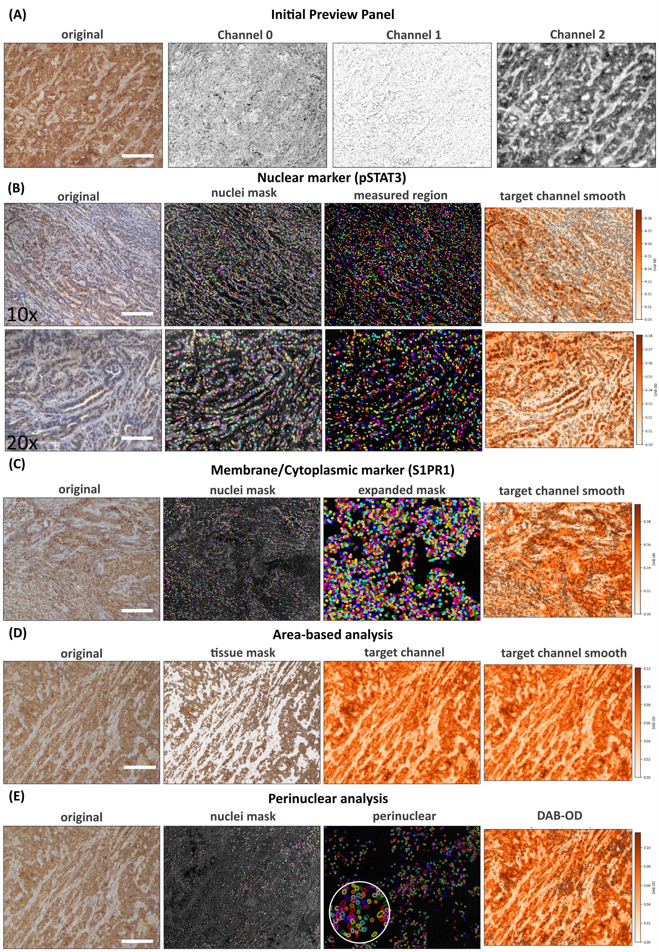
Figure 9. Panels showing different types of analysis available in the notebook. (A) Step 1 preview and (B) Step H3 segmentation output at different magnifications for pSTAT3, run using a nuclear mask and run with the nuclear option selected at Step H2. (C) S1PR1 staining after segmentation, with an expanded nuclear mask, was performed using the whole-cell analysis option set at Step H2. (D) Area-based analysis and (E) perinuclear analysis with perinuclear expansion in the inset. (D) and (E) panels are for representation only. For panels A, B, C (10×), D, and E, scale bar = 200 μm; for panel C (20×), scale bar = 100 μm.
5. Run Step H4 - Thresholds, classification, and scoring. Optical density is logarithmic with respect to transmitted light, and the pooled per-cell and per-pixel distributions are strongly right-skewed and not consistently bimodal on the native scale. Thresholds are therefore estimated on a further log10 transform, which improves separation and numerical behavior, and are reported and exported in raw optical density units.
a. Choose the threshold scope. Per marker gives each antibody its own cuts and is correct when the batch contains different antibodies, since a bright marker would otherwise set the cut for a faint one. Pooled applies one set of cuts across markers within an analysis mode and is correct when a single marker spans several conditions, because a shared cut is what makes those conditions comparable. Cell-based and area-based markers are never pooled together.
b. Choose the threshold method. The default places the negative cut by two-class Otsu on log10 optical density,
where v is the per-cell mean chromogen optical density in the selected compartment, or the per-pixel optical density within tissue in area mode. The two upper cuts are then placed at fixed offsets above it,
equivalent to 2.5 and 5 times the negative cut on the linear scale.
Note: These offsets are a reporting convention chosen during exploratory analysis. They are not derived from any physical or biological model, and the boundaries between weak, moderate, and strong staining have no formal definition in the literature.
c. From negative control: This method defines the 0/1+ boundary from the negative-control measurements rather than form the sample distribution,
where τ is the control tolerance, the fraction of control measurements permitted above the negative cut, and the two upper cuts are placed by three-class multi-Otsu [14] on the sample measurements lying above it. The remaining methods, Otsu followed by multi-Otsu above it and four-class multi-Otsu, are offered for comparison, and thresholds stored in a previous run can be imported.
d. Read the negative control panel. It reports how many control images and measurements exist for the current marker, their median and upper percentiles, and the percentage of control measurements that the current negative cut would call positive. That percentage is the false-positive rate the cut implies on tissue known to carry no target signal. It is stored with the threshold and exported.
e. Inspect the preview. The distribution view shows the pooled histogram with the cuts drawn on it; the whole-image and single-tile views show the classification applied to the image itself. Including control images in the file list classifies them with the same cuts, so anything that lights up in a control is background that the cut is failing to exclude.
f. Adjust the three sliders where the cuts do not match the staining, then press Store for this marker.
Note: Automatic thresholds are not biological defaults and do not bear any biological meaning. When analyzing, manual adjustment must be done with sliders. A live preview option can be ticked during adjustment; it regenerates the histogram/annotated images each time the user releases the mouse click. Check Figure 10 for the automatic and adjusted histogram with secondary control in the background.
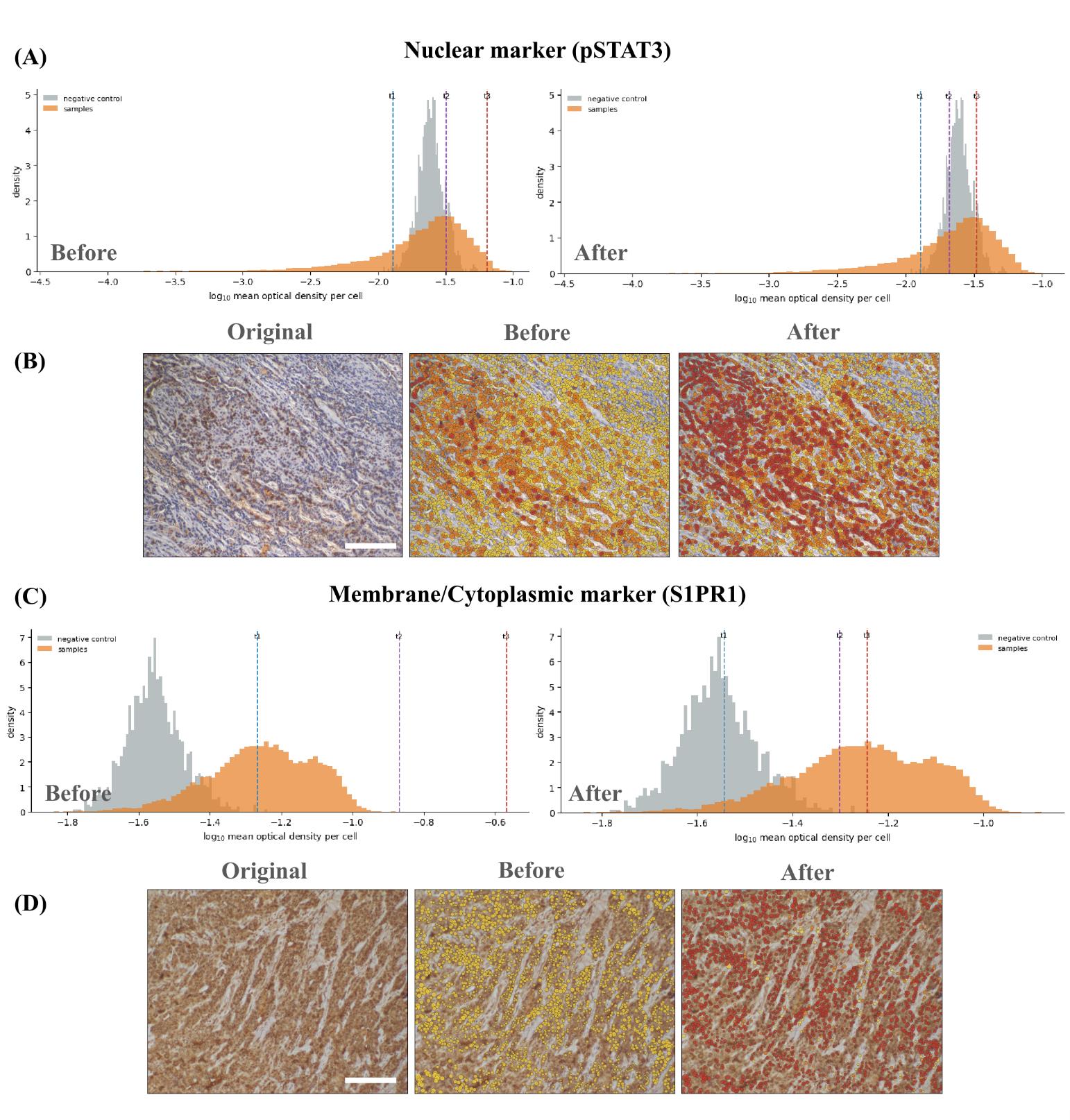
Figure 10. Manual refinement of automatically generated DAB intensity thresholds. (A) Density distributions of log10-transformed mean DAB optical density per cell for the negative control (grey) and pSTAT3-stained samples (orange). The left and right histograms show the automatically generated and manually adjusted thresholds, respectively. Dashed lines indicate the negative/weak (t1), weak/moderate (t2), and moderate/strong (t3) intensity boundaries. (B) Representative pSTAT3 image shown as the original image, the classification overlay generated using the automatic thresholds, and the overlay after manual adjustment. (C) Corresponding DAB optical-density distributions and threshold refinement for the membrane/cytoplasmic marker S1PR1. (D) Representative S1PR1 image shown as the original image and classification overlays before and after threshold adjustment. Yellow, orange, and red indicate cells classified as weak (1+), moderate (2+), and strong (3+), respectively. The optical-density measurements remain unchanged between the “Before” and “After” panels; only the classification thresholds are modified. Scale bars, 200 μm.
g. Press Apply and score all files. Each cell, or each pixel in area mode, is assigned to the negative, weak, moderate, or strong band by its position relative to the three cuts, and the file-level score is
where P1, P2, and P3 are the percentages of measured cells in the weak, moderate, and strong bands. The score runs from 0 to 300. In area mode, the same weighting is applied to area fractions rather than cell counts, and the result is reported separately as an area intensity score because a large stained cell contributes more area than a small one. Mean optical density, which requires no thresholds at all, is reported alongside both scores.
Note on interpreting the control readout: Control positivity is the percentage of negative-control measurements that exceed the negative/weak threshold. Values ≤1% are consistent with the background. Values between 1% and 5% need a visual review of the control image. Values >5% indicate that the threshold falls within the main background distribution; consequently, positive-cell fractions and H-scores calculated using that threshold should be interpreted with caution.
6. Run Step H5 - Export results. The workbook written depends on which analysis modes are run and contains Run_Metadata, Thresholds, Cell_Detail, Area_Detail, Area_Tiles, Plotting, Control_QC, and Mask_QC, with an optional per-cell sheet. Run_Metadata carries the schema and software versions, the full deconvolution matrix with its quality metrics, and every segmentation and area parameter. Thresholds carries each cut, its scope, the method that produced it, and whether a slider was moved afterward.
a. The same tables can be written as CSV files bundled in one archive. Control measurements are kept in Control_QC and never enter the sample sheets.
Critical: The automatic methods provide starting suggestions rather than universally valid biological cutoffs. Establish and document marker-specific and batch-specific thresholds using negative controls and, where possible, blinded expert assessments. The pipeline uses fixed stain vectors for the profile selected in Step H1 and performs no slide-specific stain-vector estimation, stain normalization, background correction, or scanner calibration. The resulting H-score and area intensity score are semi-quantitative and are not clinical diagnostic scores; moreover, a pathologist's scoring is the gold standard for H-DAB analysis.
Optional (extra mile): Fluorescence and H–DAB/IHC segmentation of large datasets may take considerable time. An optional ntfy webhook can be added to notify the user when a long-running Colab analysis is complete. For more information about setting this up, check the paper’s GitHub repository (https://github.com/arunviswanathan91/ImageAnalysis/blob/main/COLAB_NTFY_ALERTS.md).
import requestsNTFY_TOPIC = "your-private-topic-name"requests.post( f"https://ntfy.sh/{NTFY_TOPIC}", data="Colab analysis completed.")Data analysis
All analyses reported in this protocol were performed here. No part of the workflow has appeared in any prior research article, so the complete method is provided below rather than summarized from a publication.
Fluorescence branch
Marker-positive objects are identified when their mean intensity exceeds the user-selected threshold; Otsu, Triangle, and Yen provide descriptive histogram cut points and do not perform hypothesis testing. Double- and triple-positive populations are obtained by combining the corresponding single-marker classifications and are not mutually exclusive. Population frequency is calculated as the number of positive objects divided by the total number of segmented objects in the image or analysis group.
Morphology and fluorescence are measured from the same mask. When mask expansion or marker-guided watershed is used, area, circularity, elongation, and intensity describe the resulting cell approximation rather than the original nuclear boundary. Area is converted from pixels to square micrometers only when a physical pixel size is available. Objects smaller than the specified minimum size (15 pixels by default) are removed; border-touching objects, staining artifacts, and out-of-focus fields are otherwise retained unless predefined exclusion criteria are applied.
The notebook performs descriptive, object-level quantification but not inferential comparisons between experimental groups. Images or specimens (not individual segmented cells) must be treated as independent biological units. We recommend at least three independent biological replicates per condition, with multiple fields treated as technical or nested measurements and summarized at the specimen level. The workflow does not automatically perform background subtraction, flat-field correction, spectral unmixing, autofluorescence removal, bleed-through compensation, or batch normalization; any such processing must be validated and reported separately. We recommend at least three independent biological replicates per condition, each represented by more than one field of view or section, with the number of technical replicates stated separately. Because the unit of analysis is the image or specimen, not the cell, replication has to be built at that level. Measuring more cells within one section improves the precision of that section and adds nothing to the biological comparison.
Chromogenic branch
After color deconvolution, the quantity measured depends on the analysis mode set in Step H2. In cell mode, it is the mean chromogen optical density inside the compartment selected for that marker: the nuclear mask, a nucleus-derived perinuclear ring, or an expanded whole-cell approximation. Nuclear chromogen optical density, counterstain optical density, nuclear position, nuclear area, and measurement area are retained alongside the compartment measurement, so a nuclear and a ring result can be compared on the same cells. In area mode, it is the per-pixel chromogen optical density within the tissue mask, stored as a histogram on fixed logarithmic edges, along with the summed raw optical density in each bin, so that both an area fraction and a mean can be recovered exactly once the thresholds are set.
Threshold placement is the only statistical procedure the notebook performs on the study data, and the estimators are provided in full so that the reported cut can be reproduced. Optical density is clipped at 10-5 and log10-transformed before estimation, because the pooled distribution is strongly right-skewed on the native scale. The negative cut is then either the Otsu split of the transformed distribution, the (1 - τ) quantile of the negative control measurements, or the lowest boundary of a four-class multi-Otsu partition. The two upper cuts are either fixed offsets of 0.398 and 0.699 log10 units above the negative cut, equal to 2.5 and 5 times it on the linear scale, or three-class multi-Otsu boundaries fitted to the measurements lying above the negative cut. Estimation is refused, and the sliders are left to the user, when fewer than 100 measurements are available in the pooled sample, in the control, or above the negative cut where the upper cuts are to be fitted.
Thresholds are estimated once per scope and applied unchanged to every file and, in area mode, to every tile. Estimating them per file or per tile would redefine the bands for each image and destroy comparability across a batch. The file-level H-score is calculated from the percentages of measured cells in the weak, moderate, and strong bands, and the area intensity score applies the same weighting to area fractions. Both run from 0 to 300 and are reported under separate names because they are not the same measurement.
Where a negative control is registered, the notebook reports the proportion of control measurements that the negative cut would call positive. This is the false-positive rate the cut implies on tissue known to carry no target signal, and it is the quality-control statistic for the run. At or below 1%, it is consistent with the background. Between 1% and 5%, the cut should be re-examined against the control image. Above 5%, the cut lies inside the background distribution, and the resulting scores are not interpretable. The value, the number of control measurements supporting it, and the method used to produce the cut are written to the Thresholds sheet upon export.
A measurement is included when the compartment optical density is finite and greater than zero. In cell mode, an image that returns no nuclear labels is skipped and reported, and cells whose measurement region contains no pixels after expansion are dropped; the number dropped is printed for each file. In area mode, an image whose tissue mask is empty is skipped, and, where tiling is used, tiles below the minimum tissue fraction of 0.10 are discarded as glass or artifact. Per-pixel measurements are accumulated into 1,024 logarithmically spaced bins spanning 10-5 to 100.5, which holds the binning error on an area fraction below 0.1%, and the sum of unsmoothed optical density is carried alongside each bin so that a band mean is an exact ratio of sums rather than a bin-center approximation. Control measurements are tagged upon acquisition and excluded from every sample summary.
The statistical unit is the image or specimen, and cells from a single image are not independent biological replicates. We recommend at least three biological replicates per condition, with technical replicates reported separately, and the same measurement compartment, expansion ratio, and threshold scope applied to every file entered into one comparison. Thresholds are written to a JSON file at the end of Step H4; importing that file in a later session, rather than re-estimating, is what makes a second batch comparable to the first. Report threshold sensitivity, the control false-positive rate, failed segmentation, excluded objects, any change of measurement compartment or analysis mode, and every manual threshold adjustment.
The mean optical density is reported for each file alongside the banded score. It requires no thresholds and is the quantity to fall back on when the intensity distribution has no separable negative population. In the HER2 evaluation below, it ranked patches by pathologist grade at least as well as the H-score did, which is worth holding in view before any particular threshold is defended.
Statistical analysis used to evaluate the workflow
The agreement statistics reported in Validation of protocol were computed outside the notebook, in Python 3.12.13 with NumPy, SciPy, pandas, scikit-image, and scikit-learn. Running the protocol itself requires no programming; reproducing these statistics requires working knowledge of Python.
Agreement between a computed score and a reference grade was measured in three ways, because they answer different questions. Spearman's rank correlation and the ordinal c-index, the probability that a higher-grade image ranks higher than a lower-grade one, measure discrimination and require no thresholds. Quadratic weighted Cohen's kappa [17] and the exact four-class agreement measure grading both depend on where the band boundaries sit. The Kruskal–Wallis test was used to test whether score distributions differ across reference grades. Every agreement figure is reported together with the chance level under the mapping used and with the attainable ceiling, computed as the sum over classes of the smaller of the predicted and the observed class prevalence, since no estimator can exceed that ceiling, however well it discriminates.
Thresholds were fitted and evaluated on separate images throughout. For the HER2 evaluation, cut points were refitted inside each of five stratified cross-validation folds and applied to the held-out patches. For the Human Protein Atlas evaluation, quartile cut points were refitted on 200 stratified split halves and evaluated on the complementary half. Confidence intervals for pooled agreement were obtained via cluster bootstrapping, resampling antibodies rather than cores, because cores from a single antibody are not independent. The difference in kappa between the two measurement compartments was estimated by paired bootstrap on the images common to both. All resampling used a fixed seed.
Images were included in these analyses only when the reference label was one of the four defined classes. Antibodies with fewer than 20 usable cores, or with fewer than two distinct reference classes, were not scored. TOP2A was excluded after failing in all three measurement modes and is reported separately as an unresolved case rather than folded into the pooled estimate.
No programming is needed to run either branch. Every step is driven by widgets in the browser, and the outputs are CSV and XLSX tables that open in Excel, GraphPad Prism, R, or Python. FCS 3.1 exports open in FlowJo, FCS Express, or any conventional flow cytometry package, where an exported event is a segmented image object and not a cytometer event. Any inferential testing on the exported tables, and any attempt to reproduce the validation analysis, requires R or Python at the level of loading a table, fitting the model set out in the study plan, and reporting it.
Validation of protocol
Fluorescence branch
The technical operation of the fluorescence branch was demonstrated using a 512 × 512-pixel, 16-bit OIR image with four channels generated in-house in a murine study. The images were generated from FFPE sections of a pancreas from a genetically modified KrasG12D mouse. DAPI was designated as the nuclear channel, and CD8 and GZB as analytical markers. Because no pan-cellular channel was available, distance-based expansion was used instead of watershed. The run used an NVIDIA Tesla T4 GPU, Python 3.12.13, Cellpose 4.2.1.1, and the cpsam_v2 model. The estimated nuclear diameter was 30.0 pixels (18.6 micrometers), and the masks were expanded by 8 pixels. Measurements were obtained for 805 objects, with 27 intensity, position, morphology, and file-identification fields recorded for each object. The workflow produced CSV, XLSX, and FCS.
The same fluorescence workflow was applied to a whole-slide multiplex image containing DAPI (blue), CD8 (magenta), PD-1 (red), and VISTA (green), generated in-house in a murine pancreatic cancer study. The image was an FFPE section of the pancreas in a KrasG12D mutant mouse. Images were captured using an Olympus FV3000 confocal microscope and stitched using CellSens software after acquisition. The full-slide views and enlarged region of interest shown in Figure 11 demonstrate that the workflow can be used with larger multichannel tissue sections when the image fits within the available runtime memory. At 40× magnification, Cellpose segmentation retrieved 44,323 cells and markers from the whole-slide image. The FCS file generated from this image was analyzed, and the representative contour plots are shown in Figure 12.
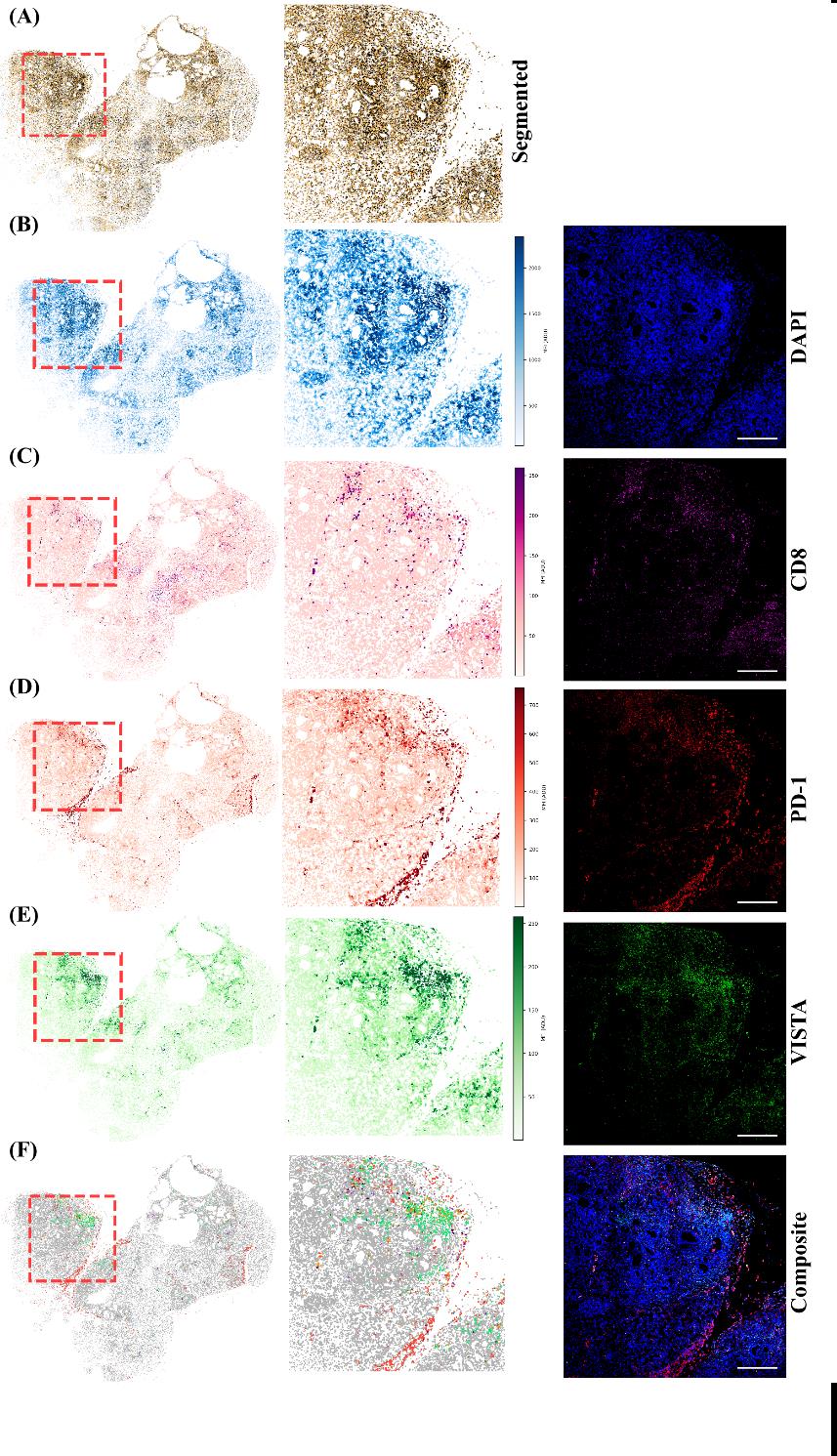
Figure 11. Multiplex whole-slide fluorescence analysis. (A) Segmented-cell map of the tissue section. (B–E) Whole-slide maps (left), enlarged boxed regions (middle), and fluorescence channels (right) for DAPI (blue), CD8 (magenta), PD-1 (red), and VISTA (green). (F) Combined marker-classification map and merged fluorescence image. Red dashed boxes indicate the enlarged region. Scale bars, 200 μm.
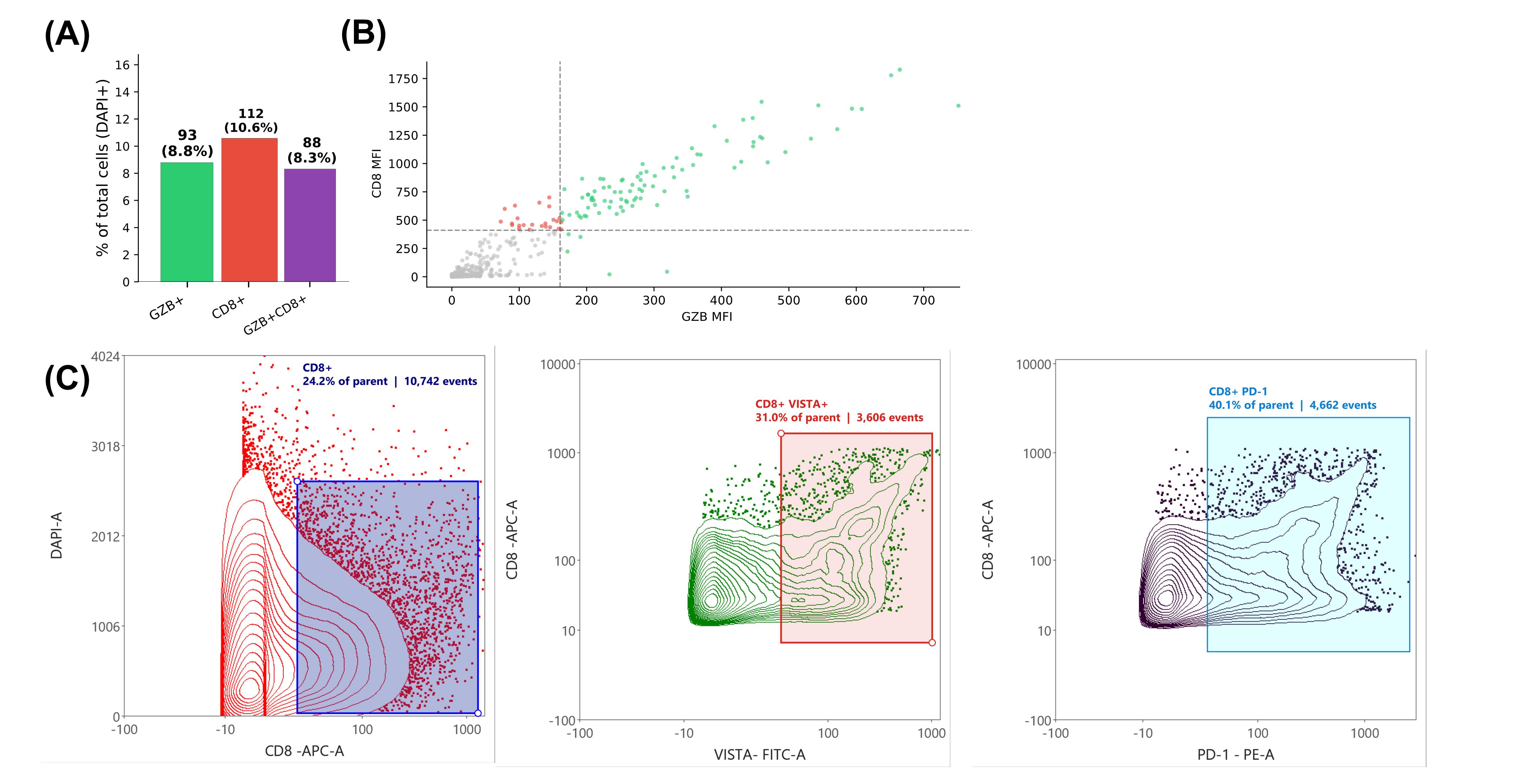
Figure 12. Image-derived fluorescence measurements from single-image and whole-slide analyses. (A) Numbers and percentages of GZB-positive, CD8-positive, and GZB/CD8-double-positive objects in a CD8/GZB-stained image acquired at 40× magnification. Percentages use all DAPI-segmented objects as the denominator, and the positive populations overlap. (B) Per-cell CD8 and GZB mean fluorescence intensities (MFI) from the same image. Dashed lines indicate the selected positivity thresholds. (C) Contour plots generated by importing the FCS file exported from the multiplex whole-slide analysis. The plots illustrate gates for DAPI-CD8-positive (left), daughter gates for CD8/VISTA-double-positive (middle), and CD8/PD-1-double-positive populations (right); annotations report percentages of the corresponding parent population and event counts. Each FCS event represents a segmented image object and was not acquired using a flow cytometer. The contour plots generated here are representative only if appropriate single-stain controls are included when the endpoint is FCS-based analysis.
External validation methodology
For external validation of the fluorescence workflow, the fluorescence workflow was independently evaluated using the publicly available 44-channel TONSIL-1 t-CyCIF image and the associated single-cell measurements reported by Rashid et al. [10]. In the original study, an FFPE human tonsil section was imaged using tissue-based cyclic immunofluorescence (t-CyCIF). The authors corrected illumination artifacts using BaSiC, stitched and registered the images using ASHLAR, segmented cells using iLASTIK and MATLAB, and extracted published single-cell features using histoCAT. These measurements served as a reference.
For independent validation, DNA1 was re-segmented using Cellpose-SAM, yielding 61,173 objects, and the raw mean fluorescence was calculated within each Cellpose mask across all 44 channels. Cellpose and published objects were paired using mutual nearest-centroid pairs; this succeeded for 55,242 objects (90.3%), indicating that spatial correspondence was established for the great majority of segmented objects. Pairs were then retained for concordance analysis only if they simultaneously satisfied a centroid-distance cutoff and an area-ratio window of 0.50–2.00 relative to the matched reference cell, yielding 17,625 high-confidence pairs. Border-touching objects were excluded, leaving 17,614 high-confidence matched pairs used in the concordance analysis below. This value, therefore, reflects a conservative joint matching criterion rather than the fraction of objects that were spatially unmatched, undetected, or affected by image registration. Published natural-log intensities and newly measured raw intensities were converted to a common log2 scale. Agreement for DNA1 and 26 biological markers was evaluated using Spearman’s correlation, Lin’s concordance correlation coefficient (CCC), regression slope, mean bias, and Bland–Altman 95% limits of agreement. Marker positivity was determined independently for the pipeline and reference measurements using Otsu thresholds. Exact binary agreement, pipeline over-call, pipeline under-call, and Cohen’s kappa were then calculated.
Fluorescence concordance with published measurements
The independently measured fluorescence values were strongly associated with the published measurements (Figure 13A, B). For CD45, Spearman’s ρ was 0.979, and CCC was 0.950, with a regression slope of 1.06 and mean bias of 0.19 log2 units. Bland–Altman analysis showed a corresponding mean difference of 0.188 log2 units and 95% limits of agreement from -0.15 to 0.53 (Figure 13C), indicating a small positive offset in the pipeline measurement. For FOXP3, Spearman’s ρ was 0.977, and CCC was 0.978, with a slope of 0.90 and negligible overall bias (-0.02 log2 units). Its Bland–Altman limits were -0.23 to 0.19 log2 units (Figure 13D); however, the negative trend at higher intensities suggests some intensity-dependent proportional disagreement despite the small average bias. Together, these findings demonstrate strong agreement with the published measurements, with a modest systematic overestimation of CD45 and near-zero average error for FOXP3, although the pipeline tended to underestimate the highest FOXP3 intensities.
The fluorescence LUT composite shows the spatial distributions of DNA1, CD45, and FOXP3; it is included for visualization only and was not used to calculate agreement statistics (Figure 13E). Representative DNA1 fluorescence and Cellpose boundaries demonstrate the quality of the independent segmentation (Figure 13G). Across DNA1 and the 26 biological markers, the median Spearman correlation was 0.977, the median Cohen’s kappa was 0.879, and the median pipeline over-call and under-call rates were 2.56% and 1.27%, respectively (Figure 13F). These results demonstrate strong technical concordance with the published single-cell measurements. Because the evaluation used a single image field from a single specimen, it does not establish biological reproducibility; however, it verifies our pipeline.
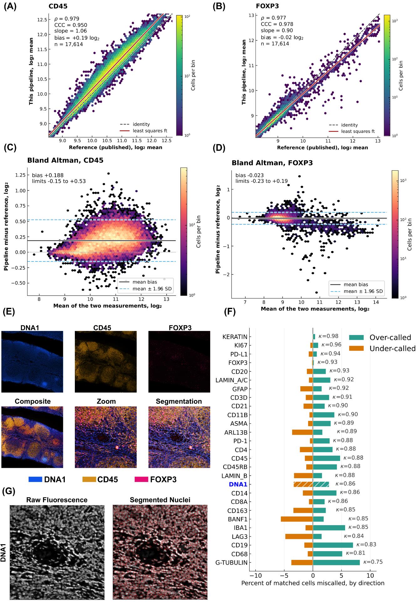
Figure 13. External validation of the fluorescence-analysis branch using a published t-CyCIF tonsil dataset. (A, B) Density scatterplots comparing log2-transformed pipeline and published mean fluorescence measurements for 17,614 matched cells for (A) CD45 and (B) FOXP3. The dashed line represents identity, the red line represents the least-squares regression fit, and color indicates the number of cells per hexagonal bin. (C, D) Bland–Altman plots for (C) CD45 and (D) FOXP3. The solid black line indicates the mean pipeline-minus-reference difference, and the dashed blue lines indicate the 95% limits of agreement calculated as the mean difference ± 1.96 standard deviations. (E) Representative pixel-level LUT visualization of DNA1, CD45, and FOXP3, including the individual channels and additive composite. LUT scaling was used only for visualization. (F) Marker-specific pipeline over-call and under-call rates after independent Otsu thresholding of pipeline and reference measurements. Teal bars represent pipeline-positive/reference-negative objects, orange bars represent pipeline-negative/reference-positive objects, and κ denotes Cohen’s kappa. (G) Representative DNA1 fluorescence image before (left) and after (right) overlaying the independently generated Cellpose-SAM boundaries.
Chromogenic branch
The chromogenic branch was evaluated using two complementary datasets. This was necessary because quantitative DAB measurements can be affected by antibody characteristics, tissue processing, staining protocol, batch effects, the type of DAB system used, image acquisition, and color response. HER2-IHC-40x provided a balanced single-target benchmark with four pathologist-assigned grades, allowing measurement compartments and thresholding strategies to be compared under a defined grading task. The Human Protein Atlas (HPA) evaluation provided a broader challenge across different antibodies, subcellular localizations, cancer types, and staining distributions. Together, the evaluations assess performance within a controlled HER2 task and transportability across more heterogeneous IHC applications; they do not constitute formal interlaboratory or clinical validation.
HER2-IHC-40x validation methodology
The first evaluation used the HER2-IHC-40x dataset [15]. Duplicate filenames were removed from the source archives, leaving 10,991 usable RGB patches of 1,024 × 1,024 pixels. A fixed-seed, class-balanced subset of 4,000 patches was selected, comprising 1,000 patches from each pathologist-assigned HER2 grade: 0, 1+, 2+, and 3+ (Figure 14). Because the Zenodo-distributed archive’s own train and test partitions were found to overlap (20,937 cataloged files reduced to 10,997 unique filenames after deduplication), the original partition was not used, and all deduplicated patches were pooled before the balanced 4,000-patch subset was drawn.
Nuclei were segmented from the hematoxylin component using the pretrained Cellpose-SAM cpsam_v2 model, automatic diameter estimation, a flow threshold of 0.40, a cell-probability threshold of 0.0, and a minimum mask size of 15 pixels (Figure 14). DAB optical density was measured separately within 548,551 nuclear objects and 545,891 nucleus-derived perinuclear regions generated using an expansion ratio of 0.5. For each compartment, cellular staining was categorized as negative, weak, moderate, or strong, and patch H-scores were converted to predicted grades using fixed thresholds of 10, 50, and 150.
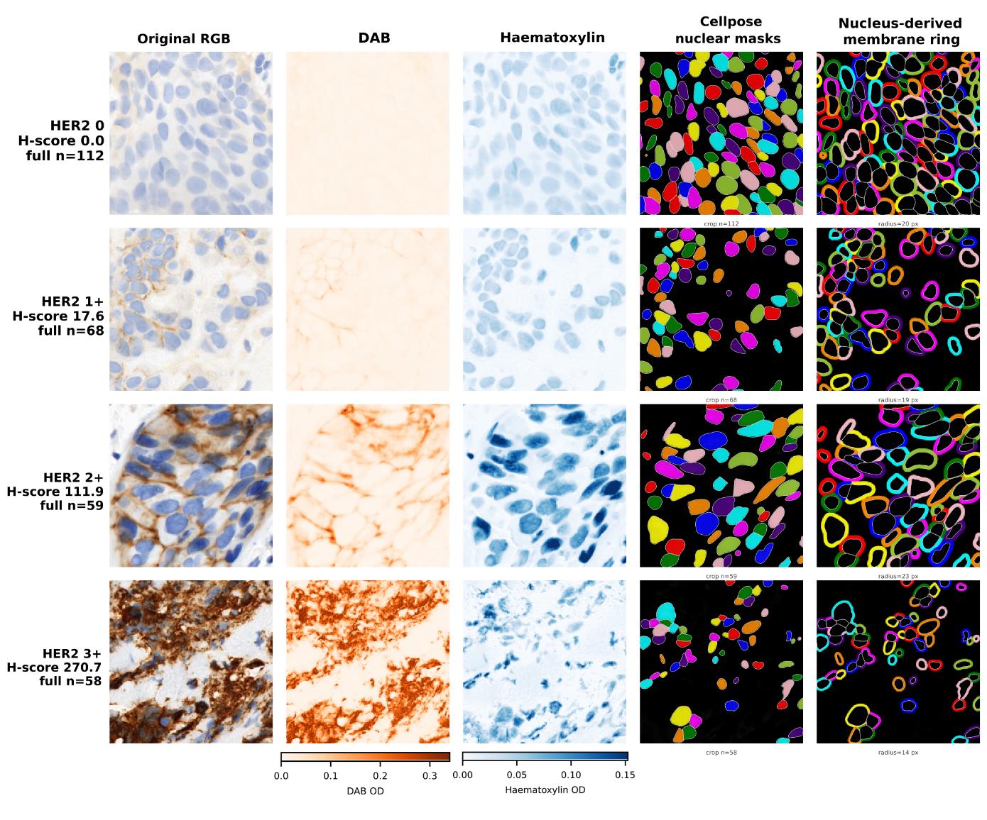
Figure 14. Representative HER2 immunohistochemistry images and compartment-specific segmentation. One image was selected from each pathologist-assigned HER2 category (0, 1+, 2+, and 3+) based on proximity to the median perinuclear-ring H-score for that category. Columns show the original RGB image, DAB and hematoxylin optical-density components, Cellpose nuclear masks, and nucleus-derived perinuclear rings. The rings were generated by collision-aware expansion of each nuclear mask, excluding the nucleus; the expansion radius is shown for each image. DAB and hematoxylin images use shared display scales across all four categories, and display normalization does not alter the optical-density values used for analysis. The reported H-scores were calculated from full-image perinuclear-ring measurements, and n indicates the number of segmented nuclear objects in the full image.
Five intensity-threshold rules were compared. The rule implemented in the pipeline estimated the negative/weak threshold by two-class Otsu thresholding of log10-transformed DAB optical density and placed the remaining thresholds at fixed log offsets. Thresholds were refitted within each of five stratified cross-validation folds and applied to the held-out patches. Quadratic weighted Cohen’s kappa [17], exact four-class agreement, within-one-grade agreement, signed grade error, and the ordinal c-index were calculated. Confidence intervals were obtained from 2,000 bootstrap replicates, and the nuclear–perinuclear comparison was evaluated using a paired bootstrap over the same patches.
HER2-IHC-40x validation findings
Cellular DAB optical-density distributions shifted progressively across the pathologist-assigned HER2 grades, although considerable overlap remained between adjacent grades (Figure 15A). This ordering was retained after aggregation to patch H-scores, which generally increased with reference grade (Figure 15B). The ordinal c-index was 0.946 for the perinuclear compartment and 0.930 for the nuclear compartment, indicating strong threshold-independent ranking of the four grades.
Under the Otsu-with-fixed-log-offsets rule implemented in the pipeline, perinuclear measurement produced 70.3% exact agreement with the pathologist-assigned grade (95% CI 68.9%–71.7%) and a quadratic-weighted kappa of 0.876 (95% CI 0.869–0.884). Nuclear measurement produced 61.2% exact agreement (95% CI 59.6%–62.7%) and a kappa of 0.822 (95% CI 0.812–0.831). On the same 4,000 patches, the paired difference in kappa was 0.054 in favor of the perinuclear compartment (95% CI 0.048–0.062). Fold-level comparisons showed that the pipeline rule and the Otsu-plus-multi-Otsu rule performed similarly, whereas four-class multi-Otsu and rules operating on linear intensity distributions produced substantially lower agreement (Figure 15C).
The confusion matrices showed that perinuclear measurement improved the classification of grades 2+ and 3+ in particular (Figure 15D). The signed-error distributions further showed that the better-performing methods predominantly produced exact classifications or one-grade errors, whereas the weaker methods generated broader patterns of under-calling or over-calling (Figure 15E). It should be noted that the intensity histograms were not manually adjusted; the thresholds were retained as determined by Otsu estimation of the background distribution and the predefined log-scale offsets. Perinuclear optical density, computed as a fixed-ratio ring expansion around the segmented nucleus, approximates but does not reproduce explicit membrane-boundary segmentation as used in conventional HER2 immunohistochemical scoring. Agreement between this measurement and patch-level pathologist-assigned grades demonstrates technical concordance with the reference labels and does not establish clinical HER2 scoring performance.
Across the evaluated methods, strong ordinal discrimination did not always translate into high exact agreement, as exact classification also depended on the positions of the fitted thresholds and the resulting predicted-grade distribution (Figure 15F). Ranking the configurations by exact agreement showed that the two perinuclear methods using log-transformed Otsu thresholds performed best and approached their attainable agreement ceilings (Figure 15G). These results demonstrate that DAB optical density retained strong ordinal information, but that categorical grade agreement depended on intensity transformation, threshold placement, and selection of a biologically appropriate measurement compartment.
Within each cross-validation fold, the initial cellular-intensity threshold was estimated from the training patches using Otsu thresholding, and the predefined log-scale offsets were used to derive the remaining thresholds. These thresholds were then applied without adjustment to the held-out patches. The small difference between in-sample and out-of-fold agreement indicates that the thresholding procedure was stable within this dataset (File S1, Figure S1); it does not establish that the resulting numerical thresholds are directly transferable to images produced using different staining batches, scanners, or laboratories.
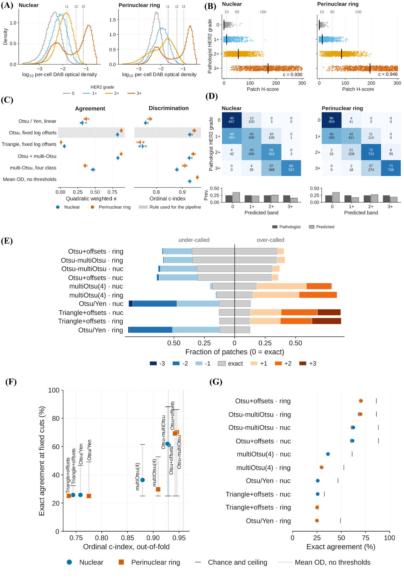
Figure 15. Technical validation of chromogenic quantification using the HER2-IHC-40x dataset. (A) Distributions of log10-transformed per-cell mean deconvolved DAB optical density for pathologist-assigned HER2 grades 0, 1+, 2+, and 3+ in the nuclear and perinuclear-ring compartments. Vertical dotted lines indicate the three cellular-intensity thresholds (t1–t3) generated by the Otsu-with-fixed-log-offsets rule. (B) Out-of-fold patch H-scores grouped by pathologist-assigned HER2 grade. Each point represents one patch, black vertical bars indicate grade medians, and grey vertical lines indicate the fixed H-score grade boundaries of 10, 50, and 150. The ordinal c-index is shown for each compartment. (C) Quadratic-weighted Cohen’s kappa and ordinal c-index for the evaluated thresholding rules. Small points represent individual cross-validation folds, larger symbols represent fold means, and the shaded row identifies the rule implemented in the pipeline. Mean DAB optical density is included as a threshold-free discrimination reference. (D) Out-of-fold confusion matrices for the pipeline rule in the nuclear and perinuclear-ring compartments. Each cell displays the row percentage and patch count; the bar charts below compare the marginal prevalence of pathologist-assigned and predicted grades. (E) Signed grade-error distributions for every thresholding rule and measurement compartment. Negative values indicate under-calling, positive values indicate over-calling, and zero indicates exact agreement; colors distinguish disagreements of one, two, or three grades. (F) Out-of-fold exact four-class agreement plotted against ordinal c-index. Vertical ranges extend from chance agreement to the attainable agreement ceiling, while dotted vertical lines indicate the threshold-free c-index obtained from mean DAB optical density. (G) Thresholding rules ranked by out-of-fold exact agreement. Blue and orange symbols denote nuclear and perinuclear-ring measurements, respectively, and grey vertical marks indicate their attainable agreement ceilings. n = 4,000 patches, comprising 1,000 patches from each reference grade.
Human Protein Atlas validation methodology
A second evaluation was performed because agreement in a single antibody and a single tissue does not demonstrate performance across the heterogeneous staining patterns encountered in IHC. The pipeline was therefore applied to 1,709 cancer tissue cores obtained from the Human Protein Atlas [16,18], representing 22 antibodies and 20 cancer types, with one selected core per patient. The HPA reference was the specialist-assigned staining-intensity category: negative, weak, moderate, or strong.
A measurement mode was assigned to each antibody before final scoring according to its annotated subcellular localization. Nuclear measurements were used for nuclear targets, and perinuclear measurements for membranous and cytoplasmic targets. Area-based measurement was used for ATP1A1 and CCND1 because the localization-assigned compartment fell below the prespecified kappa criterion of 0.40, and area measurement provided a substantive improvement. Scores were calculated separately within each antibody and converted to predicted classes using antibody-specific quartile cut points. For threshold-dependent grade agreement, cut points were fitted on one subset of images or cores and applied to a separate held-out subset, so fitting and evaluation did not use the same samples. Threshold-free measures, including the ordinal c-index and continuous fluorescence concordance statistics, did not require this separation because no cut points were fitted.
Exact four-class agreement, quadratic weighted kappa, signed grade error, and the ordinal c-index were calculated per antibody. Pooled confidence intervals were estimated using a cluster bootstrap that resampled antibodies rather than individual cores. The three measurement modes were also compared on the subset of cores available under every mode. Mode-selection optimism was estimated by selecting the best-performing mode on one half of the cores and evaluating it on the other half.
Human Protein Atlas validation findings
Core-weighted exact agreement using in-sample quartile cut points was 48.9% (95% CI 45.0%–52.8%; cluster bootstrap over antibodies), compared with 25.0% expected by chance. The pooled confusion matrix showed that most disagreements occurred between neighboring intensity grades rather than across multiple grades (Figure 16A). Overall, exact agreement was 48.3% when cut points were fitted on one subset of cores and applied to a separate held-out subset. The close agreement between the in-sample and held-out estimates indicated little overall optimism from fitting and evaluating the cut points on the same cores (Figure 16C).
Agreement nevertheless varied considerably among antibodies. The signed-error distributions show the proportions of exactly classified, under-called, and over-called cores for each antibody (Figure 16B). In-sample exact agreement ranged from 65.0% for ERBB2 and 62.8% for PTPRC to 31.6% for MKI67. Threshold-free discrimination ranged from an ordinal c-index of 0.912 for AR to 0.599 for VIM (Figure 16D). Antibodies with similar discrimination could nevertheless have different exact agreement because exact classification also depended on the fitted quartile cut points and the distribution of HPA-assigned grades. Individual plots of computational H-score against HPA-assigned intensity and antibody-specific confusion matrices across the four HPA intensity classes are provided in File S2.
The absolute difference in quadratic-weighted kappa between the assigned measurement mode and the best-performing alternative was at least 0.10 for 9 of the 22 antibodies (File S1, Figure S3). Thus, choosing a nuclear, perinuclear-ring, or area-based measurement could materially affect agreement. Selecting the best-performing mode using the same cores on which it was evaluated produced a median kappa optimism of 0.032 (interquartile range 0.016–0.049; File S1, Figure S2). Measurement mode should therefore be specified according to the known subcellular localization of the target or determined using an independent calibration dataset, rather than selected retrospectively from the evaluation results.
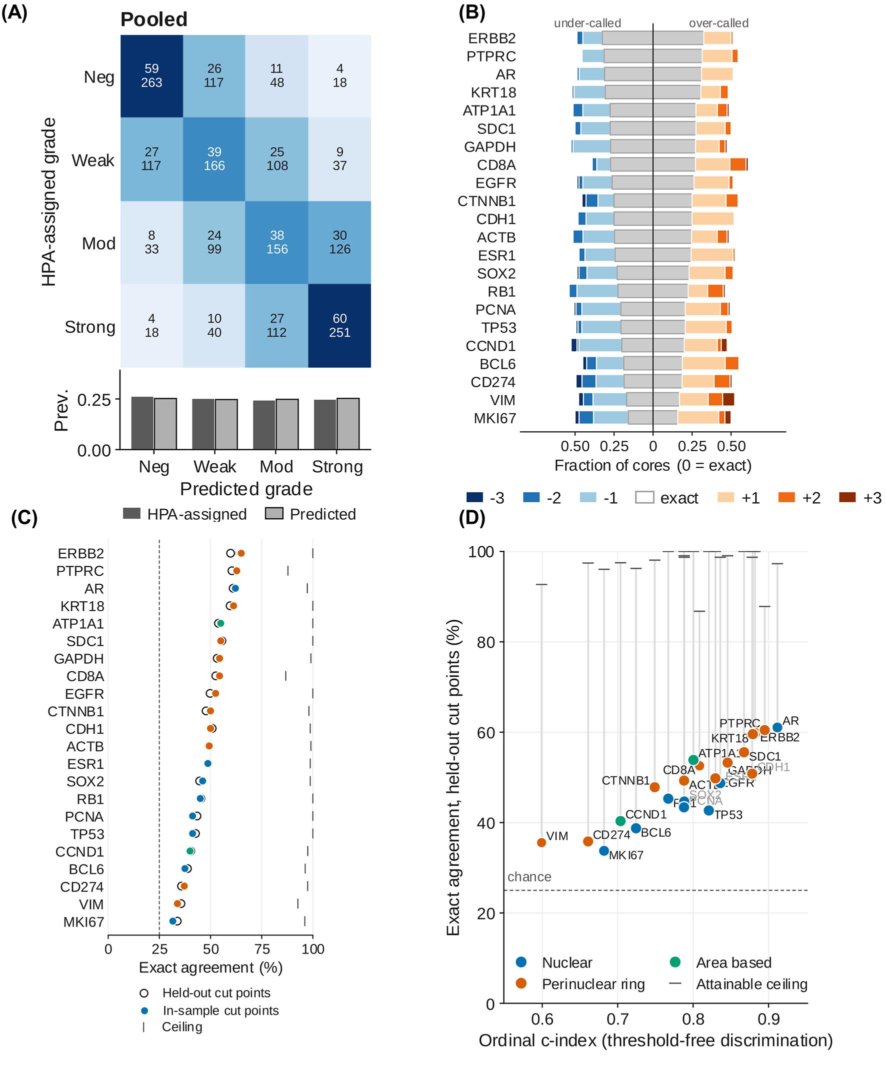
Figure 16. Agreement between computational scores and Human Protein Atlas–assigned staining intensity across 22 antibodies. (A) Distribution of signed classification errors for each antibody. The central grey segment represents exact agreement, blue segments represent under-calling by one to three grades, and orange segments represent over-calling by one to three grades. Antibodies are ordered by exact agreement. (B) Confusion matrix pooled across all antibodies, showing row percentages and core counts. The bar chart below compares the prevalence of the four HPA-assigned and computationally predicted grades. (C) Exact agreement obtained using cut points fitted on held-out cores plotted against the threshold-free ordinal c-index for each antibody. Colors indicate the assigned measurement mode: nuclear, perinuclear ring, or area-based. The horizontal dotted line indicates the 25% chance level, and the vertical grey lines extend to the attainable agreement ceiling for each antibody. (D) Exact agreement for each antibody using quartile cut points fitted on held-out cores (open circles) and in-sample (filled circles). Vertical lines show the attainable agreement ceiling, and the horizontal dotted line indicates the 25% chance level. n = 1,709 cores across 22 antibodies and 20 cancer types.
TOP2A produced a negative quadratic-weighted kappa under all three measurement modes and was reported separately as an unresolved case (File S1, Figure S4). Its mode-specific confusion matrices and representative tissue cores are provided in the Supplementary Information. DAB optical density alone did not separate the four HPA-assigned intensity classes, suggesting that a different endpoint, such as the proportion of positive nuclei, may be more appropriate for this marker.
Overall conclusion and limitations
The two evaluations support the chromogenic branch as a reproducible research workflow while defining its boundaries. In the controlled HER2 task, perinuclear measurement and log-transformed thresholding produced high ordinal discrimination and strong grade agreement. Across the more heterogeneous HPA collection, agreement remained above chance but varied substantially by antibody and measurement compartment. Therefore, measurement mode and intensity thresholds should be prespecified from target biology and independently calibrated for the antibody, staining workflow, and imaging system being analyzed.
These results constitute dataset-specific technical validation rather than clinical validation. No manually annotated nuclear masks or cell-level staining categories were available, so segmentation accuracy and individual-cell classification were not established. The HER2 archive’s original training and test partitions were combined, and multiple patches may originate from the same tissue region. This is because the distributed archive provides no patient, case, or tissue-block identifiers in its filenames or directory structure, so patient- or slide-level separation of the validation set is not possible using the released source identifiers. In the HPA evaluation, cores from each antibody represented multiple cancer types, and whole-core measurements could include stromal or non-tumor staining. The reported agreement statistics should be interpreted in light of these limitations. Established platforms such as QuPath, Fiji, and CellProfiler offer a considerably broader and more exhaustive set of options, including manual annotation, trainable classifiers, and whole-slide image management, whereas this workflow relies on pretrained segmentation models that require no training data or annotation and offers fewer analytical options, which is the trade-off for its simplicity. Table 5 consolidates the comparison between popular analysis platforms and this workflow.
Table 5. Comparison with commonly used image-analysis platforms
| Feature | QuPath | Fiji | CellProfiler | This workflow |
| Local installation | Required | Required | Required | None (Colab) |
| Workstation needed | Yes | Yes | Yes | No; browser, free GPU tier |
| Microscope formats | Bio-Formats | Bio-Formats | Bio-Formats | OIR, CZI, LIF, ND2, TIFF, PNG, JPEG |
| Whole-slide images | Yes | Memory-limited | Memory-limited | Colab-memory-limited |
| Pretrained deep-learning segmentation | Via extensions | Via plugins | Via plugin | Built-in (Cellpose, micro-SAM) |
| Custom or trained models | Yes | Yes | Yes | By code edit only |
| Mask geometry options | Cell expansion | Plugin-dependent | Secondary objects | Nuclear, distance, watershed |
| Manual annotation/correction | Yes | Yes | Yes (module) | No |
| Live threshold preview | Yes | Yes | Test Mode | Yes (Otsu, Triangle, Yen, manual) |
| Batch processing | Yes | Via macros | Yes | Yes (by file or folder) |
| Export formats | CSV, GeoJSON | CSV, TIFF, ROIs | CSV, database | CSV, XLSX, FCS 3.1 |
| Cytometry-style gating (FCS) | No | No | No | Yes (FlowJo-ready) |
| Customization | Scripts, extensions | Macros, plugins | Plugins | Editable Python cells |
| Provenance in exports | Scripts | Logs | Pipeline file | Automatic, every file |
| Data stays local | Yes | Yes | Yes | No (Google Cloud), can run locally |
| Expertise for standard use | Moderate | Moderate–high | Low–moderate | Low |
General notes and troubleshooting
General notes
1. The protocol integrates external segmentation and image-processing libraries. It does not introduce a new segmentation model.
2. Preserve original image data. Do not overwrite source files or rely solely on exported projections.
3. The fluorescence branch analyzes the first time point and a selected two-dimensional Z-projection. It is not a four-dimensional time-series or volumetric-analysis protocol.
4. Native intensity values are not normalized. Comparisons require controlled acquisition or a justified calibration/normalization method.
5. In the fluorescence branch, one mask geometry is applied to every marker channel, so compartment-specific quantification is not available there. The chromogenic branch sets the compartment and the expansion ratio separately for each marker. The biological consequence of this single mask geometry is visible in the external tonsil validation (Figure 14): median bias for membrane and cytoplasmic markers (CD20 0.202, CD45 0.179, CD45RB 0.189, ASMA 0.182, CD4 0.137, IBA1 0.136 log2) was consistently positive, whereas nuclear markers (BANF1 -0.084, KI67 -0.013, FOXP3 -0.015, LAMIN_B -0.007 log2) showed near-zero or negative bias, indicating that a single nuclear mask systematically under-captures membrane-proximal and cytoplasmic signal relative to nuclear signal (Figure S5, File S1).
6. Automatic thresholds can be distorted by outliers, unequal group sizes, batch effects, or unimodal distributions. No automatic method can locate a negative class in a distribution that has none. Use controls and inspect every histogram.
7. The chromogenic branch is semi-quantitative and is not intended for clinical diagnosis. The H-score and the area intensity score share a 0–300 range but are different measurements and must not be pooled or compared directly.
8. Colab runtimes are temporary, and free GPU access is not guaranteed. Save outputs to persistent storage before the runtime terminates.
9. Because several dependencies are installed without exact version pins, archive the full installation log and runtime version report. Revalidate after package updates.
10. The notebook is a user interface for analysis. Reproducibility depends on fixed input data, software versions, model weights, parameters, thresholds, and documented quality-control decisions.
11. Border-touching labels and other low-quality objects are not automatically excluded. Define and document object-level exclusion criteria when these objects could bias results.
12. In heterogeneous batch panels, the filtered CSV/XLSX column choices in Step 8 and the metric list in Step 10 are both constructed from the first batch dataframe; marker columns or morphology fields unique to later groups may be omitted. Check the exported schema against every input panel.
13. Some on-screen labels do not match the step names used here. The mask-expansion cell is titled Step 5A but its printed messages refer to Step 5B, and two cells refer to a Step 9 that does not exist, because batch handling is folded into Steps 2 and 3. Follow the section order in this protocol rather than the in-notebook cross-references.
14. Color choice is a reporting decision, not a display preference. Marker 1 and Marker 2 default to green and red in the composite and population figures; select an alternative pair before preparing figures for publication so that the panels remain readable to color-blind readers.
15. Whole-slide images are loaded into memory as image arrays; tile-based streaming is not implemented. Confirm that the image fits within the available RAM and GPU memory before batch analysis.
16. A negative control is the only threshold input in the chromogenic branch that does not assume the samples themselves contain a negative population. Where controls exist, register them in Step H1 and report the fraction of control measurements the chosen cut calls positive alongside every score.
17. The stain profile is fixed for a run and is not estimated per slide. No stain normalization, background correction, or scanner calibration is performed. Scores from different staining batches or scanners are therefore not directly comparable unless that comparability has been established separately.
18. Thresholds are written to a JSON file at the end of Step H4 and can be imported in a later session. Importing them, rather than re-estimating, is what makes a second batch comparable to the first.
19. Not every target can be scored by chromogen density. Where the annotated intensity difference is carried by the proportion of positive cells rather than by how darkly they stain, no choice of cut will recover it, and a different endpoint is required. TOP2A in the Human Protein Atlas evaluation is an example.
Troubleshooting
Problem 1: No GPU is detected in Step 1.
Possible cause: A CPU runtime is active, or no GPU is currently allocated.
Solution: Select Runtime → Change runtime type and request a GPU. If no GPU is available, retry later or use a paid or local runtime. Record the hardware used.
Problem 2: Step 1 ends with a session-crash message.
Possible cause: The notebook intentionally restarts the kernel after dependency installation.
Solution: Wait for reconnection and continue to Step 2. Do not rerun Step 1 in the same runtime.
Problem 3: OIR, CZI, LIF, or ND2 files fail to open in Step 2.
Possible causes: Java/Bio-Formats is unavailable, a format-specific reader failed, the file is damaged, or installed package versions are incompatible.
Solutions: Confirm Java status and the installation log, restart a clean runtime, and test a representative file. If necessary, convert a copy to OME-TIFF using a validated converter while retaining the original image and metadata. Document the conversion.
Problem 4: μSAM is unavailable after installation in Step 4.
Possible causes: The package installation timed out, or the runtime requires a restart.
Solutions: Review the installation error, restart the runtime if prompted, and rerun the segmentation cell. Use Cellpose if μSAM cannot be installed; record the engine actually used.
Problem 5: Nuclei are merged, fragmented, or missed in Step 4 segmentation.
Possible causes: Inappropriate model choice, diameter, flow threshold, cell-probability threshold, minimum size, projection, or channel assignment.
Solutions: Confirm the nuclear channel and projection, compare available models, and adjust one parameter at a time on representative images. Do not change parameters selectively by biological group without a prespecified rule.
Problem 6: Expanded masks capture background or neighboring cells in mask expansion in Step 5A.
Possible causes: The expansion ratio or watershed cap is too large, or the pan-cellular channel does not delineate boundaries.
Solutions: Reduce the ratio/cap, compare with nucleus-only masks, or use distance expansion instead of watershed. Validate the selected geometry for each marker compartment.
Problem 7: Marker-positive frequencies change markedly with small changes in threshold in Step 6.
Possible causes: The intensity distribution lacks a clear separation, controls are inadequate, or acquisition batches differ.
Solutions: Examine negative and single-positive controls, stratify by staining/acquisition batch when justified, conduct a threshold-sensitivity analysis, and report the decision rule.
Problem 8: Chromogenic scores are inconsistent across markers or batches in Step H4.
Possible cause: The automatic threshold suggestions were derived from pooled distributions that should not be combined.
Solution: Set the threshold scope to per marker and analyze compatible batches separately. Establish marker-specific and batch-specific cuts using negative controls and expert review and check the mean optical density alongside the banded score, since a difference that appears in the score but not in the mean optical density is a threshold effect rather than a staining difference.
Problem 9: The separated channels do not isolate the stains they name.
Possible causes: The stain vectors do not match the chromogen and counterstain actually used, or a custom matrix is poorly conditioned.
Solutions: Check the Step H1 preview and the reported condition number and stain-vector angles. For a brown DAB chromogen with hematoxylin, use the H-DAB profile. For any other chromogen, derive the vectors from single-stain control slides imaged on the same scanner rather than taking them from a published table.
Problem 10: The negative cut calls a large fraction of the negative control positive in Step H4.
Possible causes: The cut lies inside the background distribution, or the control does not match the samples in the staining batch, scanner, or compartment.
Solutions: Above 5%, the score is not interpretable. Switch the method to From negative control and lower the control tolerance, or raise the cut manually against the classified control image. Confirm that the control was processed in the same run and is claimed by the marker whose compartment it should represent.
Problem 11: Few or no nuclei are segmented in a chromogenic image.
Possible causes: The counterstain is faint or absent, or the section is so strongly stained that the chromogen dominates the hematoxylin channel.
Solutions: Inspect the normalized counterstain channel in the Step H3 preview. Lower the cell-probability threshold and the minimum mask size and compare models. Where the section carries no usable counterstain, set the marker to area-based instead, since cell mode has no denominator without segmentation.
Problem 12: Stained area fractions differ between images that look similarly stained in Step H3.
Possible cause: The tissue mask differs between the images, so the denominator differs.
Solutions: Check the tissue mask on the preview for each image. Adjust the tissue mask offset and confirm that glass, folds, and pen marks are excluded. Report the tissue fraction from the Mask_QC sheet alongside every area result.
Problem 13: Something is not working consistently during runtime, or the notebook is broken.
Possible cause: The Google Colab environment is constantly changing due to updates to the Python kernel. Notebook breakage or constant errors are expected in future runs. In such instances, you might have to edit the code yourself, or you can report the issue in the GitHub repository (https://github.com/arunviswanathan91/ImageAnalysis/issues). Details on how to report the issue can be found at https://github.com/arunviswanathan91/ImageAnalysis/blob/main/CONTRIBUTING.md.
Supplementary information
The following supporting information can be downloaded here:
1. File S1: Supplementary Figures S1–S5
2. File S2: Supplementary Figures of HPA analysis, confusion matrix for individual antibodies
Acknowledgments
The work is supported in part by ANRF core research grant (CRG/2021/001952 & CRG/2022/004283), ICMR EMR (2021-8415), and the BRIC-RGCB-laboratory research fund to KBH. AV was supported by a Senior Research Fellowship from UGC (No-495/ (CSIR NET JUNE 2019).
Author contributions
A.V.: Conceptualization, Methodology, Software, Protocol Development, Protocol Optimization and Validation, Formal Analysis, Investigation, Data Curation, Visualization, Writing—Original Draft, and Writing—Review & Editing. K.B.H.: Writing—Review & Editing, Resources, Supervision, Project Administration, and Funding Acquisition. All authors read and approved the final manuscript.
Competing interests
The authors declare no competing interests.
Ethical considerations
Animal experiments were approved by the Institutional Animal Ethics Committee of BRIC–Rajiv Gandhi Center for Biotechnology, Thiruvananthapuram. The fluorescence and chromogenic validation analyses used publicly available, de-identified human image datasets. Ethical approvals and consent requirements reported by the originating studies remain applicable.
References
- Stringer, C., Wang, T., Michaelos, M. and Pachitariu, M. (2020). Cellpose: a generalist algorithm for cellular segmentation. Nat Methods. 18(1): 100–106. https://doi.org/10.1038/s41592-020-01018-x
- Pachitariu, M., Rariden, M. and Stringer, C. (2025). Cellpose-SAM: superhuman generalization for cellular segmentation. bioRxiv. e651001. https://doi.org/10.1101/2025.04.28.651001
- Archit, A., Freckmann, L., Nair, S., Khalid, N., Hilt, P., Rajashekar, V., Freitag, M., Teuber, C., Spitzner, M., Tapia Contreras, C., et al. (2025). Segment Anything for Microscopy. Nat Methods. 22(3): 579–591. https://doi.org/10.1038/s41592-024-02580-4
- bioio-devs/bioio-imageio. (2026). Python. Bio IO Devs. Retrieved from https://github.com/bioio-devs/bioio-imageio (Original work published 2023)
- Linkert, M., Rueden, C. T., Allan, C., Burel, J. M., Moore, W., Patterson, A., Loranger, B., Moore, J., Neves, C., MacDonald, D., et al. (2010). Metadata matters: access to image data in the real world. J Cell Biol. 189(5): 777–782. https://doi.org/10.1083/jcb.201004104
- van der Walt, S., Schönberger, J. L., Nunez-Iglesias, J., Boulogne, F., Warner, J. D., Yager, N., Gouillart, E. and Yu, T. (2014). scikit-image: image processing in Python. PeerJ. 2: e453. https://doi.org/10.7717/peerj.453
- Ruifrok, A. C. and Johnston, D. A. (2001). Quantification of histochemical staining by color deconvolution. Anal Quant Cytol Histol. 23(4): 291–299. https://pubmed.ncbi.nlm.nih.gov/11531144/
- Google Colab. (n.d.). Retrieved August 29, 2026, from https://research.google.com/colaboratory/faq.html
- Running Kaggle Kernels with a GPU. (n.d.). Retrieved August 29, 2026, from https://kaggle.com/code/dansbecker/running-kaggle-kernels-with-a-gpu
- Rashid, R., Gaglia, G., Chen, Y. A., Lin, J. R., Du, Z., Maliga, Z., Schapiro, D., Yapp, C., Muhlich, J., Sokolov, A., et al. (2019). Highly multiplexed immunofluorescence images and single-cell data of immune markers in tonsil and lung cancer. Sci Data. 6(1): 323. https://doi.org/10.1038/s41597-019-0332-y
- Otsu, N. (1979). A Threshold Selection Method from Gray-Level Histograms. IEEE Trans Syst Man Cybern. 9(1): 62–66. https://doi.org/10.1109/tsmc.1979.4310076
- Zack, G. W., Rogers, W. E. and Latt, S. A. (1977). Automatic measurement of sister chromatid exchange frequency. J Histochem Cytochem. 25(7): 741–753. https://doi.org/10.1177/25.7.70454
- Yen, J.-C., Chang, F.-J. and Chang, S. (1995). A new criterion for automatic multilevel thresholding. IEEE Trans. Image Process. 4(3): 370–378. https://doi.org/10.1109/83.366472
- Liao, P. S., Chen, T. S. and Chung, P. C. (2001). A Fast Algorithm for Multilevel Thresholding. J Inf Sci Eng. 17(5): 713–727. https://doi.org/10.6688/JISE.2001.17.5.1
- Md Serajun, N., Mohammad Faizal, A. F., Hezerul Bin, A. K., Phaik Leng, C., Seow Fan, C., Lai Meng, L. and University, M. (2025). HER2-IHC-40x: High-Resolution Histopathology Image Dataset for HER2 Scoring in Breast Cancer. Zenodo. https://doi.org/10.5281/zenodo.15179608
- Uhlen, M., Zhang, C., Lee, S., Sjöstedt, E., Fagerberg, L., Bidkhori, G., Benfeitas, R., Arif, M., Liu, Z., Edfors, F., et al. (2017). A pathology atlas of the human cancer transcriptome. Science. 357(6352): eaan2507. https://doi.org/10.1126/science.aan2507
- Cohen, J. (1968). Weighted kappa: Nominal scale agreement provision for scaled disagreement or partial credit. Psychol Bull. 70(4): 213–220. https://doi.org/10.1037/h0026256
- Uhlén, M., Fagerberg, L., Hallström, B. M., Lindskog, C., Oksvold, P., Mardinoglu, A., Sivertsson, Ã., Kampf, C., Sjöstedt, E., Asplund, A., et al. (2015). Tissue-based map of the human proteome. Science. 347(6220): e1260419. https://doi.org/10.1126/science.1260419
Article Information
Publication history
Received: Sep 8, 2026
Accepted: Oct 28, 2026
Available online: Nov 19, 2026
Published: Dec 5, 2026
Copyright
© 2026 The Author(s); This is an open access article under the CC BY-NC license (https://creativecommons.org/licenses/by-nc/4.0/).
How to cite
Viswanathan, A. and Harikumar, K. B. (2026). A Validated Interactive Google Colab Workflow for Segmentation and Quantitative Analysis of Multiplex Immunofluorescence and Chromogenic Immunohistochemistry. Bio-protocol 16(23): e5890. DOI: 10.21769/BioProtoc.5890.

 Download Citation in RIS Format
Do you have any questions about this protocol?
Post your question to gather feedback from the community. We will also invite the authors of this article to respond.
 Post a Question


