


- Protocols

- Articles and Issues
- For Authors
- About
- Become a Reviewer


A Simplified Workflow for 3D Segmentation of Mouse Embryo Nuclei Using Biom3D

(§Technical contact: herve.alegot@uca.fr) Published: Vol 16, Iss 22, Nov 20, 2026 DOI: 10.21769/BioProtoc.5878 Views: 31
Reviewed by: Raniki KumariShensheng ZhaoAnonymous reviewer(s)
 PDF
 Ask a question


Protocol Collections
Comprehensive collections of detailed, peer-reviewed protocols focusing on specific topics



Abstract
Three-dimensional segmentation of cell nuclei is a fundamental step in quantitative studies of morphogenesis and early embryonic development, enabling the analysis of cellular organization and behavior in complex biological tissues. However, accurate segmentation of densely packed nuclei in large volumetric microscopy datasets remains technically challenging, as touching or closely apposed nuclei are frequently merged by instance-based segmentation approaches. Several deep learning–based approaches have been developed to address this problem, including convolutional neural network architectures and shape-based segmentation methods. Although these techniques have improved segmentation performance, their adoption is often limited by complex software installation procedures, demanding dataset annotation requirements and computational expertise. Here, we present a user-oriented workflow for 3D segmentation of nuclei in mouse embryos designed to simplify and speed up image annotation, requiring little manual intervention. The protocol combines a dual-channel imaging strategy, in which a high-resolution channel optimized for nuclear boundary detection is used to generate ground-truth annotations, while a lower-resolution DAPI channel serves as the training input. Rather than Cellpose, which is difficult to train and slow in 3D, or StarDist, which is difficult to use without programming skills, we suggest training Biom3d in its default nnCore version. The workflow includes semi-automated generation of training datasets, model training and evaluation through a preconfigured Biom3d environment, and application of the trained model to new volumetric datasets. Automated preprocessing, prediction, and post-processing steps are integrated into the pipeline to facilitate high-throughput analysis. The trained model was evaluated with a Dice score of 0.81. This protocol provides an accessible and reproducible solution for non-specialist users by minimizing manual annotation efforts and eliminating most software configuration requirements. The combination of dual-channel training data generation and a preconfigured deep learning framework enables scalable and robust 3D nuclear segmentation with limited computational expertise.
Key features
• Semi-automated generation of 3D nuclear ground-truth annotations using dual-channel fluorescence imaging and automatic segmentation of nuclear envelopes.
• End-to-end workflow covering dataset preparation, model training, evaluation, prediction, and downstream quantitative analysis of embryo imaging data using a Fiji macro.
• Preconfigured Biom3d nnCore environment requiring no programming skills and minimal deep-learning expertise for model training and deployment.
• Optimized for densely packed nuclei in fixed mouse preimplantation and peri-implantation embryos acquired by confocal microscopy.
Keywords: 3D nuclear morphology Deep learning
Image analysis
Nucleus
Biom3d
nnCore
Dual-channel imaging
Graphical overview
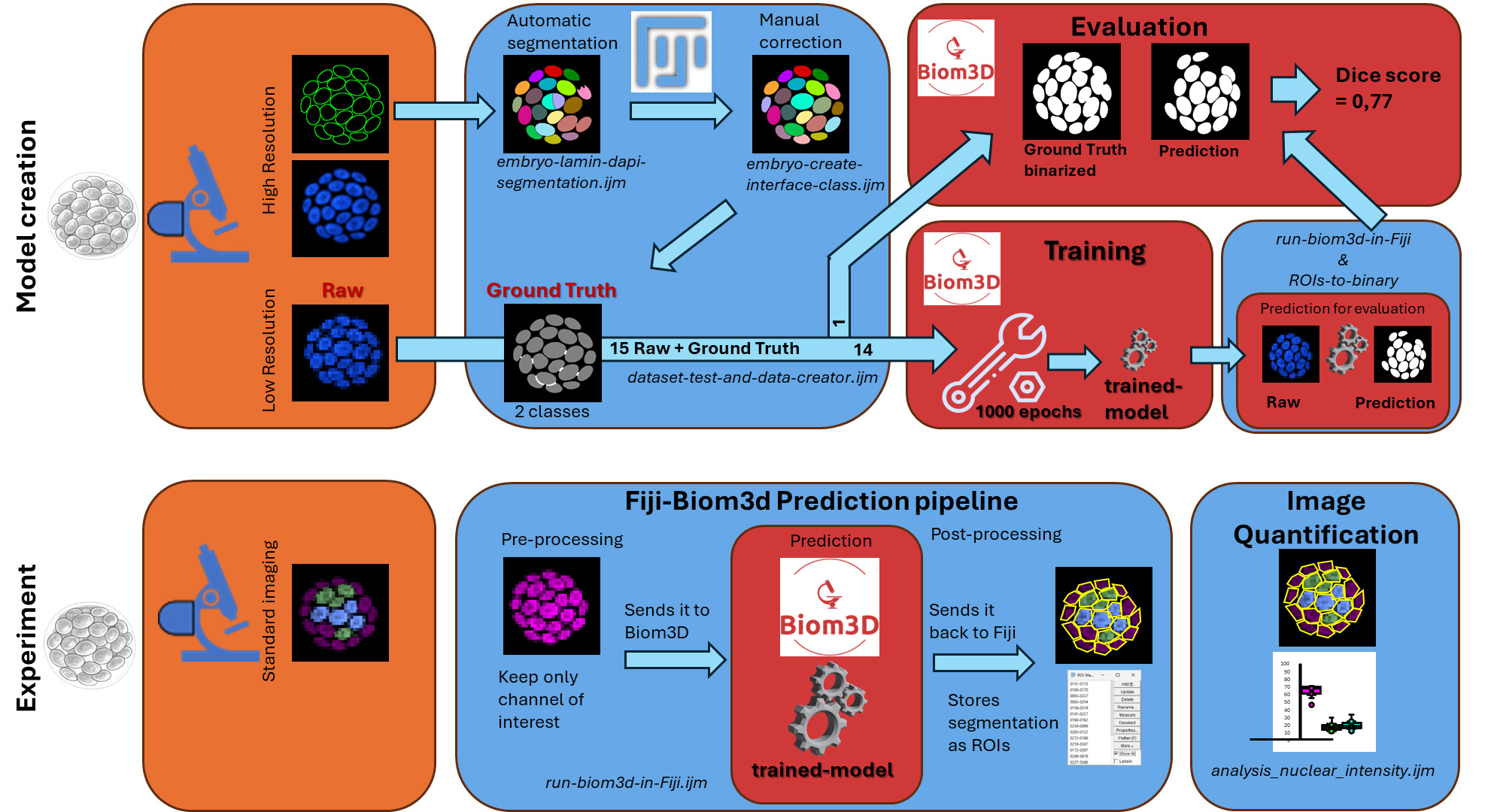
Workflow from the embryo to nuclei masks. The protocol consists of two parts: the creation of a dataset to train and evaluate a model (Model creation), and the segmentation of nuclei in an experiment of biological interest (Experiment). The left side represents the sample preparation steps, which include the immunostaining of the lamina for the training dataset and the selection of antibodies for the experiments. In orange boxes, the acquisitions for the training dataset include high-resolution images. In blue boxes are two workflows using Fiji, with various macros listed in italics and the .ijm file extension. Red boxes are the sections pertaining to the Biom3d deep learning software. The protocol includes quantification of the segmented images to evaluate the procedure.
Background
Three-dimensional imaging has become an essential tool for studying morphogenesis, embryonic development, and tissue organization at cellular resolution. Quantitative analysis of these datasets requires accurate segmentation of individual nuclei, which serves as the basis for cell counting, lineage reconstruction, spatial organization studies, and measurements of gene expression or signaling activities. However, segmentation of densely packed nuclei in volumetric microscopy datasets remains challenging because of heterogeneous fluorescence intensity, variable nuclear morphology, and close cell–cell contacts, especially in some samples like early embryos or embryoid bodies.
Recent advances in deep learning have substantially improved 3D nuclear segmentation. Convolutional neural network–based approaches and shape-based segmentation algorithms, such as Cellpose [1] and StarDist [2], can achieve high segmentation accuracy in complex biological samples. In the specific context of mouse embryo imaging, QCA-Net [3] has become a reference tool, combining a nuclear segmentation network with a nuclear detection network followed by marker-based watershed post-processing to separate touching nuclei. Nevertheless, the adoption of these methods by experimental biology laboratories remains limited. Existing workflows often require extensive manual annotation, complicated software installation procedures, management of multiple software dependencies, and manual tuning of preprocessing and training parameters, which are exacerbated by the reproducibility crisis in published software: Out of 104 published deep learning–based nuclei segmentation methods, only 6 are accompanied by source code, documentation, necessary computing environment, and training datasets (including Cellpose, StarDist, and QCA-Net) [4]. Finally, creating a training dataset, which involves manually labeling images to establish ground truth, often proves too time-consuming for the user. These requirements can represent a significant barrier for researchers without computational expertise.
The protocol presented here addresses these limitations through two complementary innovations. First, it uses a dual-channel imaging strategy [5] in which a high-resolution nuclear-envelope marker enables semi-automated generation of ground-truth annotations, substantially reducing the manual effort required to create training datasets. Second, it relies on the Biom3d framework [6] in its preconfigured nnCore mode, which provides automated preprocessing, model configuration, training, and prediction within an environment designed for non-programmer users. In a previous benchmark, nnCore demonstrated accuracy on par with the aforementioned software to segment plant nuclei [6], along with ease of use for non-experts, which is why we chose to include it in this workflow.
Compared with previously published workflows, this protocol reduces the technical expertise required to develop and deploy custom deep learning models while maintaining the flexibility to train models on user-generated datasets. Annotation, dataset creation, prediction, and image analysis steps include Fiji macros to help automate as many steps as possible. It is particularly advantageous for studies involving large collections of confocal images of mouse embryos, where manual segmentation would be impractical. The protocol also integrates downstream analysis tools that facilitate quantitative measurements after segmentation.
The protocol does, however, have several limitations. It was developed and validated using fixed mouse embryos imaged by confocal microscopy and therefore performs best on datasets acquired under similar imaging conditions. Model performance may decrease when applied to images generated with different microscopy modalities, staining strategies, or voxel sizes. In such cases, additional training data may be required to retrain or fine-tune the model. Although demonstrated here for segmentation of nuclei in mouse embryos, the workflow can be adapted to other biological systems provided that suitable training data are available. The same strategy could be applied to organoids, developing tissues, or other three-dimensional microscopy datasets. In addition, the dual-channel annotation approach can potentially be extended to the segmentation of other biological structures for which one imaging channel facilitates automated annotation while another represents the experimental signal of interest.
Materials and reagents
Biological materials
1. Wild-type CD1 mice (Janvier Labs, Le Genest-Saint-Isle, France; strain CD1, catalog number 7SN-SWISS-F); animals should be maintained under standard specific pathogen-free conditions according to institutional and national regulations
2. Mouse embryos collected at embryonic day (E) 3.5 and E4.5 from naturally mated CD1 mice (generated in-house)
Reagents
1. Paraformaldehyde (PFA), 16% p/v (Thermo Scientific Chemicals, catalog number: 043368.9M); store according to manufacturer’s instructions
2. Phosphate-buffered saline (PBS) 10×, liquid, OmniPur® grade (Sigma-Aldrich, catalog number: 6505-OP)
3. Triton X-100 (Sigma-Aldrich, catalog number: 10789704001)
4. Fetal bovine serum (FBS) (Eurobio, catalog number: CVFSVF00-01); store according to the manufacturer’s instructions
5. Lamin B1 antibody (B-10) is an IgG1 κ mouse monoclonal Lamin B1 antibody (Santa Cruz Biotechnology, catalog number: sc-374015); store according to the manufacturer’s instructions
6. SOX2 primary antibody in rabbit (Invitrogen/eBioscience, catalog number: 14-9811-82); store according to the manufacturer’s instructions.
7. GATA6 primary antibody in rat (Cell Signaling Technology, catalog number: 5851P); store according to the manufacturer’s instructions
8. Donkey anti-rat Alexa 488 secondary antibody (Life Tech, catalog number: A21208); store at 4 °C protected from light
9. Donkey anti-rabbit Cy5 secondary antibody (Jackson ImmunoResearch, catalog number: 711-175-152); store at 4 °C protected from light
10. Donkey anti-mouse Alexa Fluor 488 secondary antibody (Life Tech, catalog number: A21202); store at 4 °C protected from light
11. 4′,6-Diamidino-2-phenylindole (DAPI) (Sigma-Aldrich, catalog number: s9542); store according to the manufacturer’s instructions and protect from light
12. RapiClear® clearing reagent (SUNJin Lab, catalog number: RC147001); store according to the manufacturer’s instructions
Solutions
1. PBS 1× (see Recipes)
2. PFA 4% (see Recipes)
3. PBST 0.1% (see Recipes)
4. PBST 0.5% (see Recipes)
5. Blocking solution (see Recipes)
6. Primary antibody dilution (see Recipes)
7. Primary antibody incubation solution (see Recipes)
8. Secondary antibody staining solution (see Recipes)
9. DAPI 1/1000 (see Recipes)
Recipes
1. PBS 1×
| Reagent | Final concentration | Quantity or volume |
|---|---|---|
| PBS 10× | 1× | 100 mL |
| H2O | 900 mL | |
| Total | 1 L |
2. PFA 4%
| Reagent | Final concentration | Quantity or volume |
|---|---|---|
| PBS 1× | / | Up to 5 mL |
| PFA 16% | 4% | 1.25 mL |
| Total | 5 mL |
Store at 4 °C and use within 1 week after preparation.
3. PBST 0.1%
| Reagent | Final concentration | Quantity or volume |
|---|---|---|
| PBS 1× | / | Up to 50 mL |
| Triton X-100 | 0.1% | 50 μL |
| Total | 50 mL |
4. PBST 0.5%
| Reagent | Final concentration | Quantity or volume |
|---|---|---|
| PBS 1× | / | Up to 50 mL |
| Triton X-100 | 0.5% | 250 μL |
| Total | 50 mL |
5. Blocking solution
| Reagent | Final concentration | Quantity or volume |
|---|---|---|
| FBS | 10% | 500 μL |
| PBST 0.1% | / | Up to 5 mL |
| Total | 5 mL |
6. Primary antibody dilution
| Reagent | Final concentration | Quantity or volume |
|---|---|---|
| Primary antibody: α GATA6 or αSOX2 | 1/100 | 1 μL |
| Blocking Solution | / | Up to 100 μL |
| Total | 100 μL |
Store for up to 1 week at 4 °C.
7. Primary antibody incubation solution
| Reagent | Final concentration | Quantity or volume |
|---|---|---|
α GATA6 dilution 1/100 α SOX2 dilution 1/100 | 1:1,000 (αGATA6) 1: 3,000 (αSOX2) | 1 μL GATA6 (1/10th) 0.3 μL SOX2 (1/30th) |
| Blocking solution | / | Up to 10 μL |
| Total per well | 10 μL |
8. Secondary antibody staining solution (for 300 μL)
| Reagent | Final concentration | Quantity or volume |
|---|---|---|
| Secondary antibodies | 1:300 | 1 μL each |
| Blocking solution | / | Up to 300 μL |
| Total | 300 μL |
9. DAPI 1/1000
| Reagent | Final concentration | Quantity or volume |
|---|---|---|
| DAPI | 1:1,000 | 1 μL |
| Blocking solution | / | Up to 1 mL |
| Total | 1 mL |
Laboratory supplies
1. iSpacer, 50 μm thickness (SUNJin Lab, catalog number: IS315)
2. Terasaki plate (Thermo Scientific, catalog number: 163118)
Equipment
1. Laser scanning confocal microscopy (CSLM) (Zeiss, LSM980 with Airyscan 2, with 40× N.A.1.3 and 63× N.A.1.4 objectives).
Note: Several instruments can be used, such as laser scanning confocal microscopy (CSLM) or confocal spinning disk microscopy. The important thing is to use a lens with a high numerical aperture (NA) of 1.3–1.4. The microscope should also be equipped with high-end sensitive photodetectors or a digital camera (e.g., sCMO) with high sensitivity (high quantum efficiency, low e-read noise) suited for low-level signal acquisition in the spectral range of the fluorescent probes.
2. Computer (Dell, model: Precision 7670)
a. OS: Windows 11 Pro (x86_64/AMD64) or macOS 14 (Sonoma). If you are on Windows, you can consider that you are on “x86_64” architecture. However, if you want to confirm, open a terminal by entering “cmd” in the search bar and press Enter. Then, paste “echo %PROCESSOR_ARCHITECTURE%” and press Enter. If it prints AMD64, you are on x86_64. If not, your computer is not compatible with the installation method given here; refer to the Biom3d documentation (https://biom3d.readthedocs.io/en/latest/installation.html). On macOS, you should be on the “arm64” architecture (since M1). However, if you want to check, click the Launchpad icon in the Dock, type “Terminal” in the search field, then click Terminal. Then, paste “uname -m” and press Enter. If it prints arm64, you are on the correct architecture. If not, your computer is not compatible with the installation method given here; refer to the Biom3d documentation.
b. CPU: Intel Core i7-12800HX (or i5-12600HX) and an allocated computer memory of at least 16GB RAM (64-bit).
c. RAM: 32 GB DDR5 (64-bit, minimum 16 GB).
d. GPU: NVIDIA RTX A5000 (16 GB VRAM, CUDA 12.x) or Apple MacBook Pro (M2 Pro/Max, arm64). If you do not know the CUDA version, Biom3d will automatically detect it if it is compatible. Biom3d will automatically check your GPU for compatible CUDA versions; however, if you want to check before trying to install it, follow this process:
Open a command prompt, paste “nvidia-smi,” and press Enter. If the command is not recognized, it means that you do not have an Nvidia GPU; otherwise, it displays something similar to Figure 1.
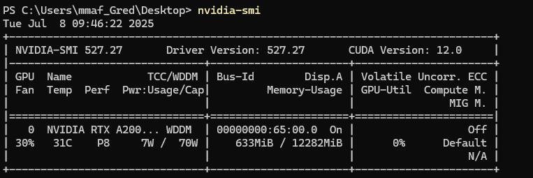
Figure 1. Result of the command “nvidia-smi” in a command prompt. The CUDA version is written in the top-right corner.
The CUDA version is written in the top-right corner of the header. The VRAM is written in the second column on the second line (without counting the header); here, 12282 MiB, so 12 GB.
Disk space: Biom3d will require 3 GB without a GPU or 7 GB with a GPU; but take into account the sizes of image datasets and future trained models.
Below the minimum system requirements, the software Biom3d may still function depending on the size of the images (dimensions and number), with longer processing times. Biom3d runs without a GPU, but the performance is significantly improved with a compatible GPU.
Software and datasets
| Type | Software/dataset/resource | Version | Date | License | Access (free or paid) |
|---|---|---|---|---|---|
| Image datasets | dataset | 2025 | CC-BY | Free | |
| Fiji | Software | 1.54p | G.P.L. | Open source | |
| Biom3d | Software | 0.0.40 | G.P.L. | Open source | |
| MorpholibJ plugin | Software | 1.6.5 | G.P.L. | Open source | |
| Omero batch plugin | Software | 2.1.1 | G.P.L. | Open source |
1. Fiji/ImageJ [7]. Fiji is just ImageJ with some useful modifications. It is an open-source image analysis software. https://Fiji.net/software/fiji/downloads
2. Default Biom3d framework nnCore: Biom3d is an open-source deep learning framework to segment 2D and 3D images [6]. Its default version, nnCore, can be installed with all dependencies using an installer function. https://github.com/GuillaumeMougeot/biom3d. Permanent link: https://archive.softwareheritage.org/browse/origin/directory/?origin_url=https://github.com/GuillaumeMougeot/biom3d.
3. MorpholibJ plugin [8]: The MorpholibJ plugin is a very useful plugin. It is a collection of mathematical morphology methods and plugins for ImageJ.
4. Omero_batch-plugin [9]: The Omero Batch Process plugin allows treating a dataset with a Fiji macro in a batch process. The image manager OMERO [10] is not required here. Version used here: 2.0.2. https://github.com/GReD-Clermont/simple-omero-client. Permanent link: GReD-Clermont/omero_batch-plugin: 2.1.1 | Zenodo
5. Download the following Fiji Macros from the folder “macros”: https://github.com/GReD-Clermont/biom3d-mouse-embryo-training
6. Seven datasets are available on a public repository of Université Clermont Auvergne: https://doi.org/10.18145/t2dq-1j51
Procedure
A. Sample preparation and image acquisition
Each experiment was performed in accordance with French and European guidelines for the care and use of laboratory animals (APAFIS #26479). Animals were housed in a specific pathogen-free facility (EOPS) with access to standard food and water, with a 12-hour light cycle, at a temperature between 20 and 26 °C and humidity of 30%–70%. All embryos used in this study were produced by natural mating. The morning of the vaginal plug was considered the E0.5 stage. Wild-type embryos were derived from the CD1 mouse strain (Janvier Labs). Beyond stage E4.5, embryos were implanted and were therefore harvested by dissection of the uterine horns, after sacrifice of the animals by cervical dislocation.
A1. Staining of nuclei in fixed tissues for training dataset production and segmentation prediction
1. Fix E3.5 and E4.5 mouse embryos in 4% PFA diluted in PBS 1× overnight at 4 °C or for 30 min at room temperature.
2. Wash for 5 min twice in PBST 0.1%.
3. Permeabilize embryos for 3 min in a solution of PBST 0.5%.
4. Block nonspecific sites in blocking solution for 1 h.
5. Incubate embryos overnight at 4 °C with the appropriate primary antibodies according to the dataset (training or prediction) diluted in 30 μL of blocking solution in a Terasaki plate:
a. For the training dataset, only antibodies against Lamin B are incubated.
b. For the prediction dataset, there is no lamina labeling. We propose here to incubate antibodies against GATA6 and SOX2. Other antibodies may be used by experimenters depending on their biological questions.
6. Wash three times for 5 min in 0.1% PBST and then incubate with 1/300 diluted secondary antibodies (anti-mouse AF488 and anti-rabbit Cy5) and 1/1,000 DAPI in blocking solution for 1–2 h at room temperature.
7. For clearing, wash three times for 10 min in PBST 0.1%.
8. Mount between the slide and coverslip with 50 μm iSpacer in 4 μL of RapiClear®.
Note: RapiClear® was not used for the training dataset.
A2. Image acquisition
In our work, we used the Airyscan 2 detector in the fast-Airyscan mode on an LSM980 microscope with an objective N.A.1.3 (40×) (Zeiss). This protocol does not describe the procedure to capture microscopy images, as this depends on the imaging equipment; however, a few guidelines are given below to acquire datasets.
Critical: Start from the plane containing the strongest signals in each channel to adjust the power of each laser and the gain of detectors before acquisition to obtain a full dynamic range, avoiding detector saturation. Each embryo is imaged entirely in a Z-shape, with signal-free planes before and after.
1. Acquisition of the training dataset: For each embryo, capture two types of image stacks with different pixel sizes: the “high-resolution” image stack and the “low-resolution” image stack:
a. High-resolution image stacks: Acquire with voxel sizes x, y, and z of 0.08 × 0.08 × 0.19 μm, in multichannel mode to capture Lamin-coupled GFP (488 nm laser) and DAPI (405 nm laser) signals. This acquisition allows automatic segmentation of the nuclei using the GFP channel to obtain the ground truth mask without the need for numerous manual corrections. Note: High-resolution DAPI imaging is recommended; although time-consuming and of no use for subsequent automated steps, it can sometimes be helpful in facilitating subsequent manual corrections.
b. Low-resolution image stacks: Acquire in the DAPI channel alone under routinely faster experimental conditions. Keep the setting identical to those for the first image, with the exception of voxel size, which is lower: 0.21 × 0.21 × 1 μm. These different voxel sizes will entail a scaling step during the creation of the training set, but optimize the time of acquisition and computing.
Critical: The high-resolution masks will be downscaled to become the ground truth mask of the low-resolution image; thus, it is important that low-resolution image stacks are taken with settings as close as possible, comprising field of view and z-stack thickness, to facilitate downscaling.
2. Acquisition of the experimental dataset: The experimental dataset should be taken with settings as close as possible to the low-resolution training dataset. This implies the voxel size and dynamic range of the DAPI channel. The number and nature of other channels and staining do not matter, since preprocessing of the experimental dataset will be applied before making predictions. Keep the same microscope and low-resolution settings (pixel size 0.21 × 0.21 × 1 μm).
B. Software installation
B1. Fiji installation
This step will be quickly performed for advanced users of Fiji, but may require some investment for inexperienced users. However, Fiji is a versatile and user-friendly environment that, once installed, allows many other applications other than the one described in this protocol. It is recommended to store Fiji in your user space rather than in Program Files.
1. Download Fiji (https://Fiji.net/software/fiji/downloads). Then, proceed with the installation. Update Fiji by selecting Help/Update Fiji in the Fiji bar menu.
2. Set up Fiji memory to a minimum of 1,700 MB by selecting Edit/Options/Memory & Threads. Fiji can be run under Windows, Mac, or Linux systems with a 64-bit OS and a 64-bit version of Java.
B2. Installation of plugins OMERO Batch Process and MorpholibJ
Note: It is recommended to install plugins via the Fiji menu update in order to benefit from the latest versions.
1. Open Fiji by double-clicking on Fiji-windows-x64.
2. Select Help > Update… from the menu to start the updater.
3. Click on Manage > Update sites. This brings up a dialog where you can activate additional update sites.
4. Activate the IJPB-plugins update site, click Apply, and close the dialog. Now you should see an additional .jar file for download.
5. Click Apply changes and restart Fiji.
6. Check that MorpholibJ is proposed in the list in the Plugin menu.
7. Select Help > Update… from the menu to start the updater.
8. Click on Manage Update sites in the new window.
9. Click on Add Unlisted Site.
10. Add https://omero.igred.fr/Fiji as the URL and GReD in the name in the second opened window.
11. Click on Apply and Close; the second window is closed.
12. Click on Apply changes and restart Fiji.
13. Check that Batch process is proposed in the menu Plugin/OMERO.
B3. Biom3d installation
While Biom3d works on Windows, Linux, and macOS, the installation method used here is only available on Windows 10/11 and macOS 14. If you want to use other installation methods, please refer to the Biom3d documentation.
1. Go to the Biom3d GitHub, Release (on the right), and select the last version; it should contain several downloadable elements. Select the “Biom3d_Windows_x86_64.zip” or “Biom3d_MacOS_arm64.zip” depending on your operating system and processor architecture. It will download an archive in .zip format.
2. This archive contains a folder named "Biom3d” (Windows) or “Biom3d.app” (macOS); extract that folder to a destination you chose. The extraction speed will depend on the hardware you have, but it takes at least 8 min. Biom3d is now installed; however, a final step must be done before using it with Fiji.
3. Start Biom3d; in Windows, double-click on the “Biom3d.bat” file in the folder; on macOS, double-click on the folder. At the first launch, Biom3d will initialize itself, check your GPU, and update itself to match your GPU. It will open a terminal window.
a. It will display “First launch detected, initializing the virtual environment” and initialize; it should take 3 min.
b. (Only on Windows) It will display “Checking for installed version of CUDA and installing appropriate PyTorch.”
i. If it fails, it displays “No CUDA compatible with Biom3d found.” If you are sure you have a compatible GPU, contact your IT support.
ii. Otherwise, it displays “Found CUDA [version], reinstalling PyTorch” and will reinstall the PyTorch dependency; it should take 3 minutes. Then, it displays “Done.”
c. It starts Biom3d Graphical User Interface (displaying “Starting Biom3d...”). Every time you use “Biom3d.bat” or “Biom3d.app,” it will skip steps B3.1–2 and directly start the Graphical User Interface.
4. (Optional) You can create a shortcut for future use. Refer to your operating system documentation for that.
C. Producing masks for the training set
One macro and a visual check/correction will be applied to the high-resolution images. Segmentation will be performed on the Lamin-GFP channel alone, using local minima to binarize images and classify voxels into background (class 0) and mask (class 1). A third class (2) will be associated with voxels marking the separation between two nearby nuclei not individualized by segmentation.
C1. Prepare high-resolution images
The high-resolution images to be processed must first be grouped together in an input folder; the acquisition channels must be in the same order, and an output folder must be created. The input folder contains raw images or, like here, processed images because of the use of the Airyscan detector in fast mode. Raw images have two channels in the owner format or .tiff. The output images will be in .tiff format with three channels: Lamin-GFP, DAPI, and label.
C2. Use the “embryo-lamin-dapi-segmentation.ijm” macro
1. Open Fiji.
2. Click on Plugins > Omero > Batch Process and fill in the window to indicate the paths to the input folder and to the embryo-lamin-dapi-segmentation.ijm macro (Figure 2).
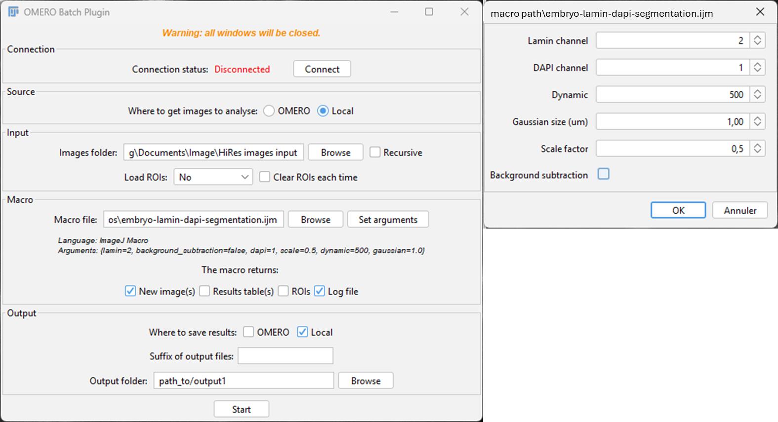
Figure 2. Snapshot of the OMERO Batch Process plugin in Fiji. On the left: Main window of OMERO Batch Plugin; Images folder, Output folder, and macro file path must be set up. In the case of the embryo-lamin-DAPI-segmentation macro, the “New image(s),” “Log file,” and “Local” boxes must be ticked. On the right: Window opened with Set arguments; parameters used for our dataset.
3. Select New Image to save the image result; select Log file to save the settings used as a .txt file.
4. Click on Local to answer the question Where to save results. Indicate the path of the output folder.
5. Click on Set arguments and fill in the new window: Lamin channel = 2; DAPI channel = 1; Dynamic = 500; Gaussian size = 1; Scale factor = 0.5.
Critical: The parameter values are appropriate for the associated training dataset but may differ for other images. If over-segmentation (i.e., objects are split), increase Dynamic; decrease it if there is sub-segmentation (objects are not separated). If not satisfactory, move Gaussian Blur in the same way (generally between 1 and 10). Dynamic is an integer between 0 and 65,535 for a 16-bit image, and between 0 and 255 for an 8-bit image. The selection of the Dynamic value depends on the intensity of your object; in our case, the intensity inside the Lamin staining is close to 0. The scale factor needs to be <1.
6. Click on Start.
Critical: The macro is written for a 2-channel image; if more or fewer channels are present, the macro will return an error.
What does the macro do?
Several steps are required to generate a good segmentation of the Lamin channel. First, an “Enhance contrast” is applied to increase the signal from the “higher” z-sections where the signal is lower. Images are then rescaled to speed up the process. If needed, the background is subtracted. A Gaussian Blur is applied, and extended minima are detected. These minima will serve as a “seed” for the watershed step. Objects touching the edges are excluded, the image is rescaled back to the original size, and the composite image containing DAPI, Lamin, and label channels is created.
C3. Check the segmentation and correct the label channel
Manual corrections:
1. Open Fiji.
2. Open an image from the output folder.
3. Click on Image > Color > Split Channels. Channels need to be split because of the main correction needed for the MorpholibJ label edition tool, which works with only the label channel. After correcting some errors, you may compare with the actual DAPI or Lamin channels; in this case, merge the channels back in Image > Color > Merge Channels... and select the “C3...._edited” version of your label image. You may need to do some back and forth from the composite image to the label edition tool.
4. Check the masks and corresponding raw image in z (synchronize windows in z with Analyze > Tools > Synchronize windows. The DAPI channel sometimes helps to select:
• Unlabeled nuclei: We decided not to try to draw a missing nucleus since it would take too long and, in our experience, it doesn’t impact the training.
• Non-nuclei objects: Go to Plugin > MorpholibJ > Label Images > Label Edition. Select the multipoint tool, click on the label(s) you want to delete (you can delete more than one at a time), and press “Remove selected.” When you are done, press Done.
• Split nuclei: Go to Plugin > MorpholibJ > Label Images > Label Edition. Select the multipoint tool, click on the labels you want to merge, and press Merge. When you are done, press Done.
• Fused nuclei: Click on the brush icon and switch colors with the color picker tool to Black/White, then select the brush tool and erase the voxels of touching nuclei (in x, y, and z). The aim is to remove any connection between voxels of each nucleus. Then, go to Plugin > MorpholibJ > Binary Images > Connected Components Labeling. The touching nuclei should have different colors; if this is not the case, try to remove a bit more voxels and retry. If you have too many objects, nearby nuclei may share the same color but still have different labels. To check, put your cursor on one object and look at its value in the bottom of the Fiji main panel. Then, check if the other object has a different value: this means it is a separate object.
5. Merge back your channels in Image > Color > Merge Channels... and select the last edited label image as channel 3.
6. Save the image in an “output2” folder and open the following image until the end of the output folder. Representative examples of wrong segmentations are given in Figure 3.
Note: In our hands, we never obtained “Fused nuclei,” illustrating the interest of the Lamin signal in separating nuclei from each other. With other data, this situation could arise. The non-nuclei objects were the most common corrections. This automatic segmentation method generally leads to the detection of the whole embryonic cavity as an object; moreover, at the top and bottom of the stack, a lot of objects are detected outside the embryo. It is particularly important to remove these objects, as they are not nuclei and, using the Label Edition tool, it is quite fast (tens of seconds), whereas drawing one object in 3D is really tedious (a couple of minutes). If too many small objects are drawn after the first step, try increasing the Dynamic value.
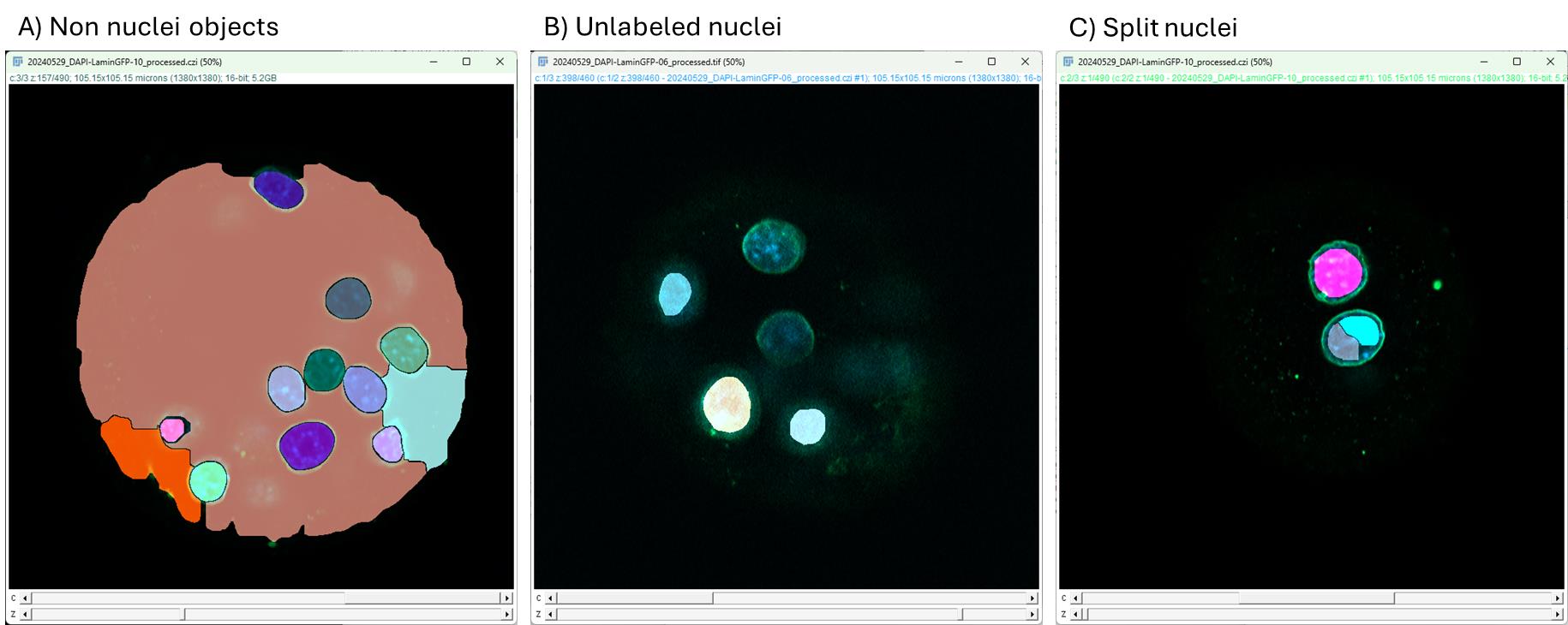
Figure 3. Typical wrong segmentations in mouse embryos. Screenshots of Fiji windows with masks generated from low-resolution DAPI images taken with the embryo-lamin-dapi-segmentation.ijm macro. Yellow stars indicate the wrong segmentation areas. (A) Three segmented regions that do not correspond to cell nuclei. They can be removed easily. (B) Two non-segmented nuclei. We chose not to correct this error because it would take too much time. See General note 5. (C) A nucleus splits into two and can be fused easily. Note: We did not find fused nuclei.
C4. Post-processing: “Embryo_create_interface_class” macro
The Embryo_create_interface_class macro will automatically create a class of voxels that are at the interface between nearby nuclei. It is based on successive dilation/erosion steps. The input folder is now the previous output2 folder.
1. Open Fiji.
2. Click on Plugins > Omero > Batch Process and fill in the window to indicate the paths to the input folder (output2) and to the “create-three-classes” macro.
3. Select New Image to save image results.
4. Click on Local to answer the question Where to save results. Click on Browse and indicate the path of a new output folder (output3). You can create the folder at this step.
5. Click on Start.
C5. Rescaling between high-resolution and low-resolution images
High- and low-resolution images do not have the same number of planes. For a high-resolution mask to become the ground truth mask of the low-resolution image, all planes must be scaled and checked for coincidence with the low-resolution image. So, we must check that no small z-shifts remain between planes after rescaling (Figure 4).
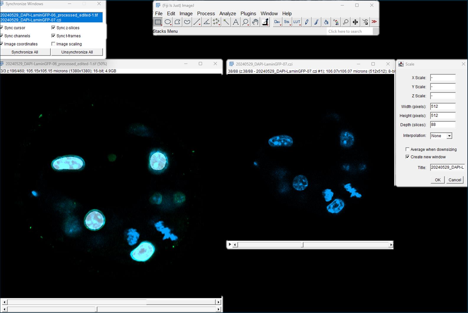
Figure 4. Rescaling of the high-resolution mask. Using the Scale tool in Fiji, the high-resolution image (left) is scaled to the low-resolution image (right).
1. Open Fiji.
2. Click on Analyse > Tools > Synchronize windows. Check all boxes except same scaling.
3. Open the first high-resolution mask in the output 3 folder and its corresponding raw low-resolution image (DAPI-channel) in this order.
Critical: By opening the files in this order, the mask will not change its name until the end of the process and can be saved without changing the name.
4. Select the mask before clicking on Image > Scale. In Width (pixels), Height (pixels), and Depth (slices), enter the number of pixels and slices of the low-resolution image. Choose interpolation: None; check box create new window.
Critical: It is important NOT to tick the box Average when downsizing since it will change the masks. Do not change the title; click Ok.
5. Synchronize the low-resolution raw image and the rescaled mask by clicking Synchronize All in the Synchronize Window.
6. Check the coincidence between signals in raw and masks, especially at the beginning and the end of the stack (Figure 5). If there is a shift, remove or add a plane to the beginning of the stack by clicking Image > Stack > Delete Slice or Image > Stack > Add Slice, respectively.
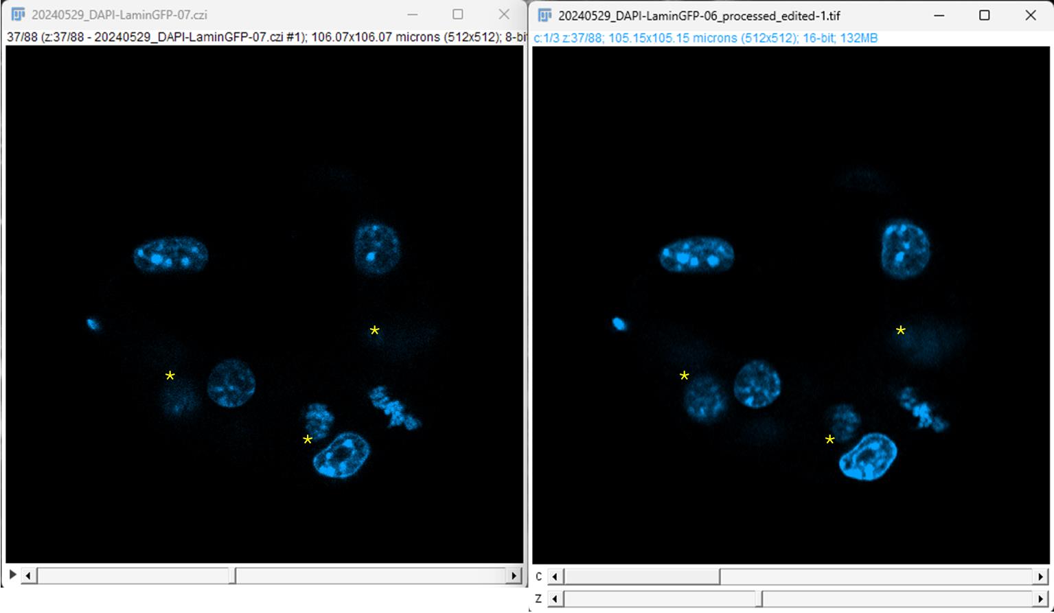
Figure 5. Check the coincidence between signals in the low-resolution and rescaled images. Original low-resolution image is on the left, displayed here at plane 37/88; the rescaled image is on the right and presents the same number of planes (to check). Both images are synchronized in z. *Note that the signal coincidence is not perfect; this is an illustration of tolerance in the coincidence between the planes. In the right image, only channel 1 is displayed; channel 2 corresponds to the Lamin labeling, and channel 3 corresponds to the rescaled mask.
7. Compensate for an added slice at the beginning by removing a slice from the end of the stack and vice versa.
8. Split channels (Image > Color > Split Channels) and keep only the mask image (“C3-”).
9. Save the mask in an output4 folder and rename the low-resolution image (remove the prefix “C3-”).
10. Close the images and open the following until the end of the folder.
C6. Organize data in folders (put aside some images for evaluation)
The raw image and its corresponding mask must have exactly the same name. The number of files should be exactly the same in the containing folders. To check, use the “Find-mismatch” macro. Your output4 folder must be renamed “mask,” and the low-resolution image folder must be named “raw.”
1. Open Fiji.
2. Click on Plugins > Macro > Run and open the Find-mismatch macro.
3. Any file that does not have a corresponding file in the other folder will be written in the log window. This macro is based on the number of files in both folders. If you have the same number of files but with different names, the macro will not find them. You need to keep at least one pair of raw/mask to evaluate the trained model before making predictions. Here, we keep one pair of images in a “to_eval” folder. In this work, we wanted to evaluate only the prediction of class 1. Class 2 needs to be removed, so we simply apply a threshold with value 1 to keep only class 1.
D. Training Biom3d
D1. Training
1. Open the Biom3d Graphical User Interface by navigating to the folder where you installed it and double-click on “Biom3d.bat” (Windows) or “Biom3d.app” (maOS), or use a previously created shortcut.
2. Click on the Start locally button.
3. Click on the Preprocess & Train tab (Figure 6).
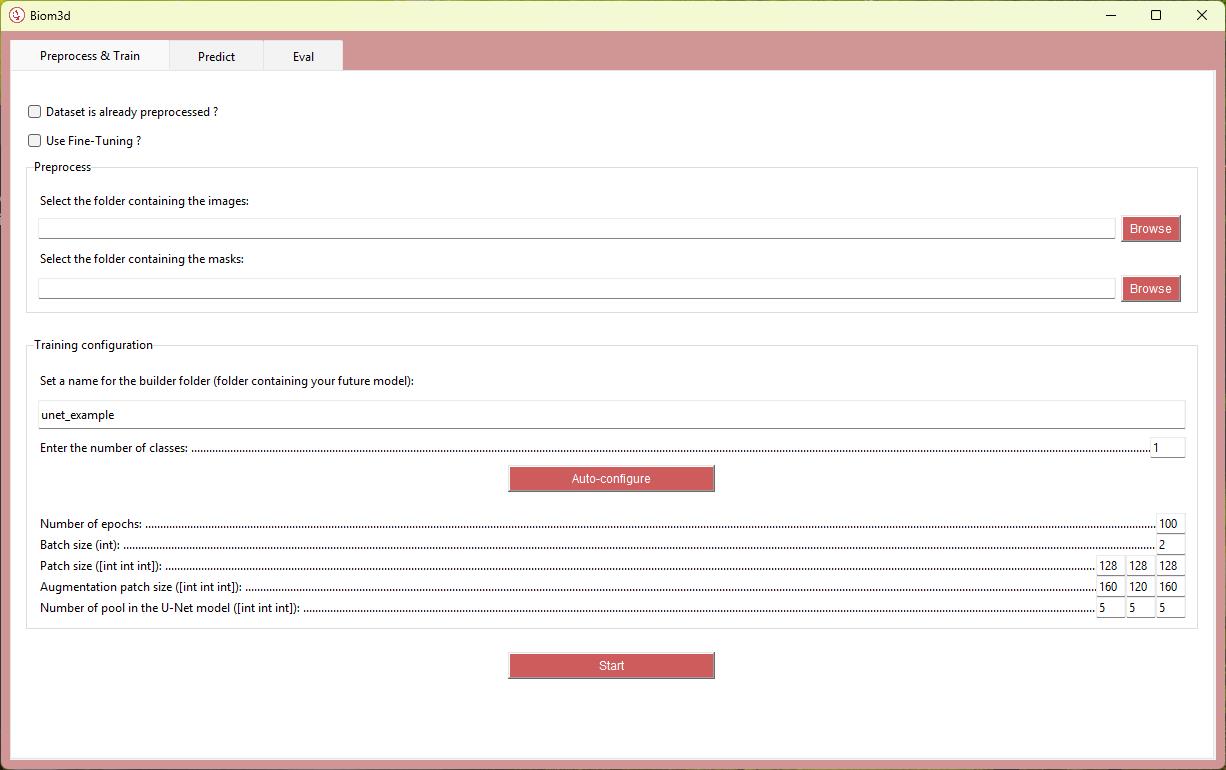
Figure 6. Biom3d Interface. Open in the Preprocess & Train tab, showing default settings that will change after the autoconfiguration process.
4. Enter the folder paths in the appropriate cases.
5. Enter a name for your model.
Note: Spaces in folders’ names generally lead to crashes. We recommend using dash (-) and underscore (_) characters only.
6. Enter Parameters: Number of classes = 2.
Notes:
1. Only certain types of objects are counted as classes; in our case, the nucleus (class = 1) and the boundaries between nuclei (class = 2). Since the background category has a class of 0, it is not counted. Click on Auto-configure (Figure 6). Four parameters are automatically calculated in the interface: Batch size, Patch size, Augmentation patch size, and Number of pool in the U-Net model. The Auto-configure function also automatically divides the training dataset between learning set and test set. See General note 6. Number of epochs = 1000.
2. It can be difficult to choose the number of epochs when you lack experience. Biom3d automatically saves the “best” model and the latest model. The best model is the first one to achieve the highest Dice Score (see step D3), and it is the one that will be used by default for predictions, thereby avoiding overfitting issues. It can be helpful to check at which epoch this best model was obtained after training to avoid waiting too long for future training runs. If this best model was obtained at 160 epochs, there is no need to run 1,000 epochs next time (assuming the same number of images and computing environment).
7. Click Start.
Note: The training time depends on the number of epochs, the image size, and the number of images. See General note 6.
What you obtain:
After the preprocessing step, after pressing Auto-configure, two folders are created: a “mask_out” and a “raw_out,” corresponding to “mask” and “raw” folders with the preprocessed images. A “configs” folder is created containing the preconfiguration file with different parameters.
After the training, you get a “fg_out” folder containing images in a Python-specific format. The model is stored in the “logs” folder, where you find a subfolder with the date and name of the model. Inside, there is an “image” folder containing small .png images of the prediction after each epoch. An epoch refers to one complete pass of the entire training dataset through the learning algorithm. Two versions of the model are stored: the last model generated and the best model. The best model is the first model where the best Dice Score was reached. Subsequently, Biom3d will use the best model to make predictions to avoid overfitting. Lastly, there is a “log” folder containing several files, including the “log.csv.” This file contains five columns with different evaluations of the quality of the model over the epochs.
D2. Interpretation of learning curves
At the beginning of the process, the training dataset is automatically split into two parts in a way that is transparent to the user: one set of images will be used for the actual learning, while the second will serve as a test set to evaluate the model on unseen data at each epoch. During training of deep learning models, the evolution of loss and accuracy over successive iterations (epochs) provides essential information regarding the quality of learning. Two sets of curves are typically monitored: training curves (evaluated on the data used for learning) and validation curves (evaluated on the separate dataset not seen by the model).
Identify the curves:
• The training loss should progressively decrease as the model adapts to the dataset.
• The validation loss reflects the model’s ability to generalize; it should decrease in parallel with training loss during the initial epochs.
Interpret convergence:
• Proper learning is characterized by a progressive reduction of both training and validation losses until reaching a plateau (Figure 7A).
• Simultaneous stabilization of accuracy curves indicates an optimal learning regime.
Detect underfitting:
• If both training and validation losses remain high or fail to decrease substantially, the model is not capturing the underlying data structure (Figure 7B).
• This indicates insufficient model complexity, inadequate training duration, or insufficient data quality.
Detect overfitting:
• If the training loss continues to decrease while the validation loss rises, the model is memorizing the training data rather than generalizing (Figure 7C).
• This is often accompanied by a divergence between training and validation accuracy.
Select the optimal model:
• The best-performing model is typically found at the epoch corresponding to the lowest validation loss or highest validation accuracy prior to divergence.
• Early stopping or model checkpointing strategies can be employed to systematically capture this stage.
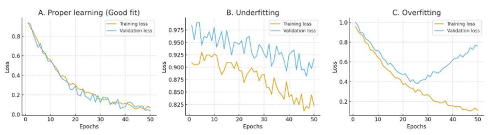
Figure 7. Examples of training curves. For each epoch, the loss functions are calculated for training and validation.
In our experiment, the training reached its best model after “only” 160 epochs, with a training loss of -0.595 and a validation loss of -0.588.
D3. Evaluation of the trained model
To evaluate the model, you need to still have at least one image and its ground truth mask in the “to eval” folder. The ground truth mask needs to be thresholded to 1 to remove interface class. Open the ground truth mask in Fiji, run Image > Adjust > Threshold and set the two cursors to 1. Press Apply, keep default parameters, and untick Calculate threshold for each image. Then, save the image, overwrite the existing one, or click Save As in a new folder but keep the same name.
Follow section E1 on the raw images and apply to the “to eval” folder (keep their masks in another folder during the prediction). Then, run the “ROIs-to-binary.ijm" macro on the folder. This will create a binary mask, comparable to the ground truth, from the ROIs. If you have many images in the folder, use the OMERO batch process plugin.
1. Open Fiji.
2. Click on Plugins > Omero > Batch Process, fill in the window to indicate the path to the “to eval” folder, and select Load ROIs > ROI Manager. Indicate the path to the ROIs-to-binary macro.
3. Select New Image to save image results. Then, compare processed masks (ground truth and predicted) with the Biom3d GUI open and in local execution:
a. Navigate to the Eval tab.
b. Fill in the path folder containing predicted masks and ground truth masks in appropriate cases.
c. Click the Start button.
What you obtain:
The answer is a number: the Dice Score. The formula of the Dice Score = 2 × (number of common voxels in a class)/(number of voxels in set predicted masks + number of voxels in set labeled masks). This is a common indicator for evaluating deep learning models. The higher it is, the better, but it depends on the quality of the training set and on the segmentation task you ask (full objects give a better Dice Score than edges). It is an indicator, but you need to check the segmented images to evaluate the model.
We evaluated the quality of class 1 only, i.e., the nuclei, because it corresponds to the signal that will be kept after processing. The accuracy of class 2 is not targeted here. Predictions and the ground truth masks are thresholded to 1 to remove class 2.
We evaluated the model with this method only on two embryos, because we only had 16 embryos from the same experiment and we wanted to use as many for the training as possible to ensure a good quality of the model.
The Dice Score value is not a sufficient indicator on its own, but can serve as a basis for other users who would like to train a model on similar types of images (e.g., acquired with a spinning disc):
• A Dice Score of 50% is not always bad; it depends on the quality of the annotation of the masks and the segmented object (relative size in the image and shape): for example, a contour that is off by one pixel will give a poor Dice Score, whereas the same filled object, because it has many internal pixels in common between the annotation and the prediction, will be much better.
• It is the end user, after visually examining the images, who decides whether the model will be able to segment the images in their study model. By overlaying the ground truth masks and the predicted masks, we can see that the nuclei are correctly segmented (Figure 8).
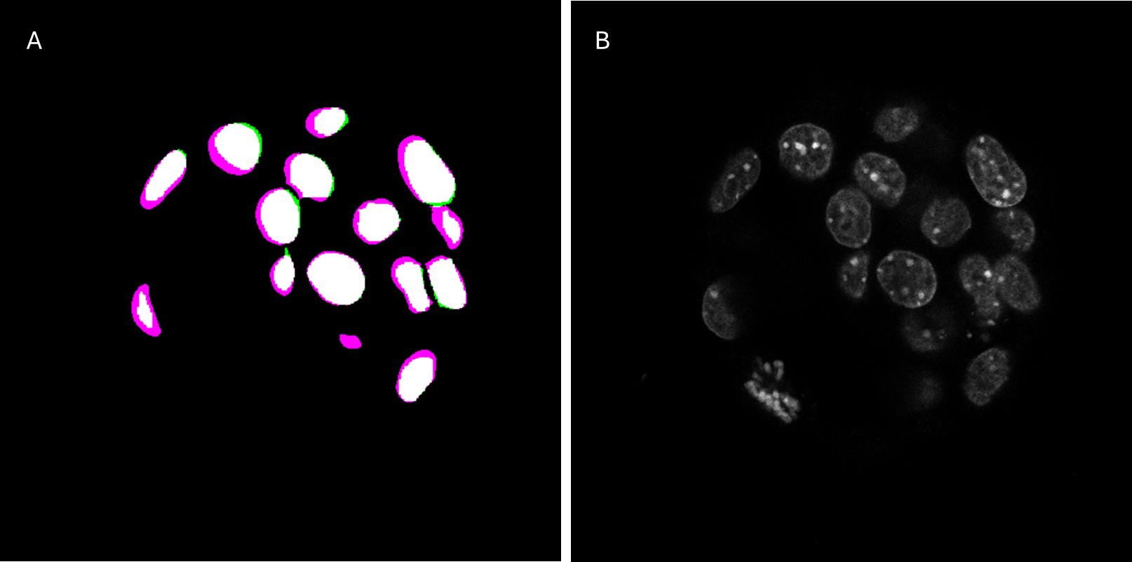
Figure 8. Comparison of the prediction and ground truth of one validation image. (A) Overlay of the prediction of the model shown in magenta and the ground truth in green. (B) Original standard-resolution image.
To complement the Dice Score, which measures voxel-level overlap, we evaluated the model's ability to separate and count individual nuclei. For the two evaluation embryos, the results are as follows: Embryo 1 showed a Dice Score of 0.79 with 59 nuclei segmented compared to 53 in the ground truth; the difference is mainly due to five missing nuclei in the ground truth that are detected by Biom3d. Embryo 2 showed a Dice Score of 0.83 with 43 nuclei detected compared to 43 in the ground truth. This dual assessment (overlap and count) provides a more robust indication of segmentation performance than the Dice Score alone. However, it is essential to examine the training curve and to check that the model is not overtrained.
E. Segmentation prediction, post-processing, and quantification
1. Open the Biom3d Graphical User Interface by navigating to the folder where you installed it and clicking on Biom3d.bat (Windows) or Biom3d.app (maOS), or using a previously created shortcut.
2. Click on the Start locally button.
3. Click on the Predict tab.
4. Enter the folder paths in appropriate cases: The folder of raw images to predict and the folder of the trained model.
5. Click on the Start button.
Note: Prediction time depends on the size and number of images and the hardware resources (GPU, RAM, etc.).
What you obtain:
A mask is created with the nuclei as the first class (voxel value of 1) and the nuclei interface as class 2 (voxel value of 2), as a .tiff file. These images are “just” raw masks and will be generated only for evaluation purposes. If you want to generate a “real” segmentation of your data of interest, go to the next section.
E1. Run the macro “run-biom3d-in-Fiji”
The model was trained on a one-channel image, so it expects to input only one channel image. However, your raw image of interest generally contains more than one channel, so we wrote a Fiji macro that preprocesses the image to keep only the DAPI channel and calls Biom3d from a Python command line. Once the prediction is done, a mask is obtained; we generally want to turn this mask into a label image (i.e., obtain an instance segmentation). The next steps are the post-processing steps. So, Fiji opens the mask and, thanks to a thresholding, the interface between nuclei (so, class 2) is removed, and the run-biom3d-in-Fiji macro does a connected component labeling, giving each separated nucleus its own identity. The results are stored as ROI in Fiji.
1. Open Fiji.
2. Click on Plugins > Omero > Batch Process and fill in the window to indicate the paths to the input folder and to the run-biom3d-in-Fiji macro.
3. Select ROI to save the image result and log to store the parameters used; also, tick the box Clear ROIs each time. You can define the parameters of the preprocessing and post-processing by selecting Set arguments.
a. First, define the path to the Python executable file. It is in your Biom3d installation folder, in Biom3d > bin > python.exe on Windows and Biom3d.app > Contents > MacOS > bin > bin > python3.11 on macOS.
b. By default, the path to the model should be in your Biom3d installation folder, in logs > date-time-name-of-the-model.
c. Define the number of the DAPI channel in your image.
d. Lastly, define a scaling factor. This factor can be useful if your image is much bigger than the training image; it helps to rescale to approximate the size of the training image.
4. Click on Local to answer the question Where to save results; it will save the ROI file and the log in the image folder.
5. Click on Start.
What you obtain:
After this step, you get an ROI file, generally as a .zip file, containing the result of the segmentation. To our knowledge, this file is usable in Fiji only and needs to be converted to labels to be able to do measurements. The next macro gives you an example of how to convert ROIs into labels, and the kind of intensity measurements that can be done.
E2. Image quantification with the “analysis_nuclear_intensity” macro
The goal of the analysis_nuclear_intensity macro is to use the previous segmentation prediction to analyze channels containing fluorescent signals. First, the macro will convert the ROIs into labels, and then the mean intensity of nuclei is measured for channels 2 and 3, corresponding here to Sox2 and Gata6.
Critical: The analysis_nuclear_intensity macro is very specific to these images, and the possibility of modification and reuse with other images is very limited. Also, the way ROIs are read implies that they have been generated by the previous macro to work.
1. Open Fiji.
2. Click on Plugins > Omero > Batch Process and fill in the window to indicate the path to the input folder and to the analysis_nuclear_intensity macro. Select Load ROIs > ROI Manager.
3. Select Results table(s) to save the result tables. Click on Local to answer the question Where to save results. It will save the result files in the image folder.
4. Click on Start.
What you obtain:
After this step, you get two tables for each analyzed image, as a .csv file: one called “Results” and the other “Numbers.” You also get two other tables, corresponding to the concatenation of all individual images. In each Results table, the nuclear mean signal intensity per channel for each cell is reported, as well as the x, y, and z positions of each cell and the volume of its nucleus. In each Numbers table, the number of cells of each type is indicated, as well as the ratio of each type over the total number of cells. To count a positive cell for each channel, a basic intensity threshold is applied and can be adjusted directly within the macro code. This last macro is just an example of how to get labels from ROIs and one way to analyze the intensity of the signal.
Result interpretation
This protocol proposes a methodology for segmenting highly dense objects within 3D images, such as mouse embryos at stages 3.5–4.5. As with any supervised deep learning method, the first step is to create a dataset with a ground-truth mask. The semi-automatic annotation based on a different staining greatly simplifies this step, which is often considered tedious and time-consuming. For this to be a real time-saver, this methodology should therefore be reserved for cases where automatic segmentation does not work or requires numerous corrections.
While corrections are certainly fewer with this technique, it is not always possible or desirable in all experiments (due to the cost of the anti-Lamin antibody, additional imaging, etc.). The contribution of machine learning techniques could be particularly advantageous.
To validate our automated nuclear segmentation pipeline on other samples, we quantified the relative proportions of primitive endoderm (PrE), epiblast (Epi), and trophectoderm (TE) cells in E4.5 mouse embryos. Sixteen embryos were dissected and subjected to immunofluorescence staining using antibodies against GATA6 and SOX2, established markers of the PrE and Epi lineages, respectively, together with DAPI nuclear staining, then imaged in 3D with a CLSM microscope. The previously trained Biom3d-nnCore model successfully segments nuclei, as can be seen on Omero (Predictions dataset, https://omero.mesocentre.uca.fr/webclient/?show=dataset-5461; see Dataset Details for instructions on viewing segmentations in Omero). Based on these predictions, we were able to determine the distribution of SOX2 and GATA6 proteins and count the number of positive cells present in mouse embryos at stage 4.5. The analysis revealed a mean total cell number of 164.8 ± 20.1 cells per embryo (mean ± SD). Lineage quantification showed that SOX2-positive Epi cells represented 16.7% ± 4.8% of total embryonic cells, whereas GATA6-positive PrE cells accounted for 19.5% ± 5.7%. The remaining 63.8% ± 8.1% corresponded to double-negative TE cells (Figure 9). These proportions are consistent with previous reports describing lineage allocation in E4.5 mouse blastocysts, respectively around 15%, 20%, and 65% [11]. Together, these results demonstrate that our approach provides an accurate, unbiased, and high-throughput method for quantifying lineage composition at the late blastocyst stage. In future experiments, this segmentation method could be used to count FISH spots or to localize them within specific cell lineages.
Since 2025, a new, very powerful deep learning method called Cellpose-SAM [12] has enabled predictions without training on 3D images. There are two reasons why our protocol remains useful: 1) Direct prediction on low-resolution DAPI images would likely require fine-tuning, but retraining Cellpose-SAM is still challenging for non-IT biologists; and 2) although Cellpose-SAM has quickly become a very popular segmentation tool for 2D images due to its efficiency and simplicity, using it for predictions based on 3D images requires a very long computation time.
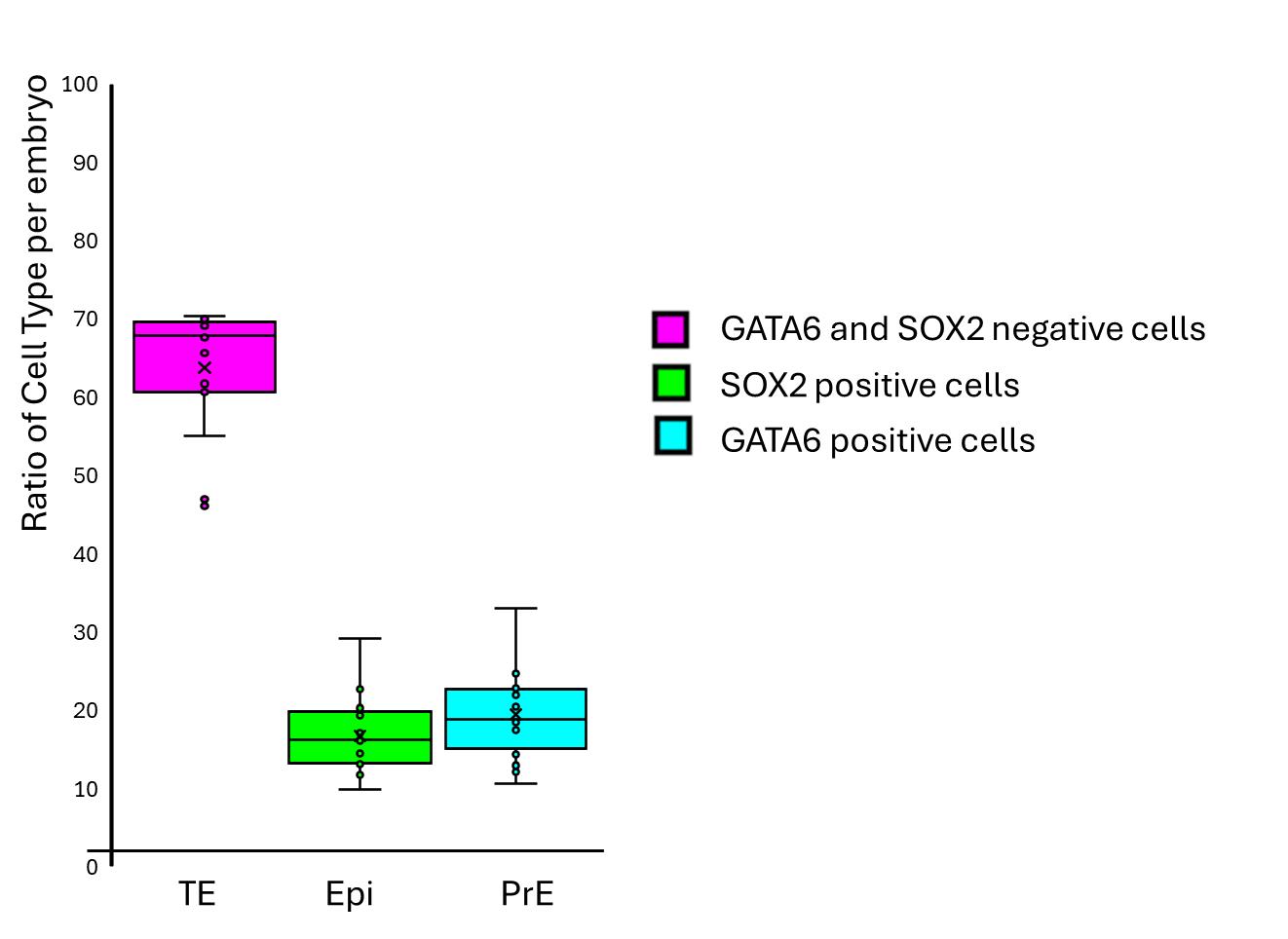
Figure 9. Distribution of cell types in E4.5 mouse embryo. 3D images of DAPI-stained mouse embryos at E4.5 with immunostaining for SOX2 and GATA6 were segmented with the run-biom3d-in-Fiji macro in the DAPI channel to quantify cell types in the whole embryo. N = 16. TE: trophectoderm; Epi: epiblast cell; PrE: primitive endoderm.
Validation of protocol
The production of the samples is detailed in Table 1.
Table 1. Summary of training, evaluation, and validation datasets. The protocol uses two distinct datasets for validation. The Evaluation dataset (2 embryos) is used for quantitative assessment of segmentation accuracy (Dice Score) by comparing predictions against ground-truth masks. The Validation dataset (16 embryos) is used to demonstrate the biological applicability of the protocol by quantifying lineage proportions (Epi, PrE, TE) in a way that is consistent with known biological patterns, without the need for ground-truth masks.
| Training dataset | Evaluation dataset | Validation dataset |
|---|---|---|
| 14 embryos | 2 embryos | 16 embryos |
| 14 image stacks | 2 image stacks | 16 image stacks |
| 789 nuclei | 105 nuclei | 2637 segmented nuclei |
| Imaged the same day | Imaged the day before, coming from the same experiment as the training dataset. | Imaged the same day, from one experiment, independent of the training and evaluation datasets. |
All data are available on the public Omero repository of Clermont Auvergne as a project and respect REMBI rules [13]. The 2026_ALEGOT project contains seven datasets:
• Three datasets for training:
“High-Resolution” dataset contains raw images used to build ground truth, Lamin and DAPI channels acquired following step A2.1a (https://omero.mesocentre.uca.fr/webclient/?show=dataset-5416).
“Training_Raw” dataset contains the DAPI-channel low-resolution images acquired following step A2.1b (/https://omero.mesocentre.uca.fr/webclient/?show=dataset-5412).
“Training_Ground-truth_Mask” dataset contains the two-class masks obtained following section C (https://omero.mesocentre.uca.fr/webclient/?show=dataset-5411).
Note that paired images (raw/ground-truth mask) have the same name. You can see all images and their ground truth. To download, select images in the central panel and click on the download arrow icon in the right panel. If the download fails, download the images in several batches.
• Three datasets for evaluation of the model: The three dataset names start with "Eval_...". They contain:
Two DAPI-channel raw images acquired following step A2.1b (https://omero.mesocentre.uca.fr/webclient/?show=dataset-5415).
Their ground truth masks, obtained following section C, plus a threshold to remove class2 (https://omero.mesocentre.uca.fr/webclient/?show=dataset-5413).
Their predicted masks, following section E (https://omero.mesocentre.uca.fr/webclient/?show=dataset-5414).
Raw images were never seen by the model during training.
• One dataset for the Result interpretation part, named "Predictions" (https://omero.mesocentre.uca.fr/webclient/?show=dataset-5461). This dataset contains original images acquired from DAPI-stained mouse embryos at E4.5 (magenta, channel 0), with immunostaining for SOX2 (green, channel 1) and GATA6 (cyan, channel 2). The masks are presented as regions of interest. To see the segmentations, double-click an image to open the viewer in a new tab, then click ROI in the upper-right corner of the right-hand panel. The segmentations appear as outlines around the nuclei. Since the outlines are barely visible, you can click on a nucleus to make it appear thicker.
The macros used in this protocol are available at https://github.com/GReD-Clermont/biom3d-mouse-embryo-training. The link to each macro is also available as a comment in the Omero right panel of the Training_Ground-truth_Mask, Eval_raw, and Predictions datasets. The Biom3d trained model is available in the attachment (right panel) of the project (https://omero.mesocentre.uca.fr/webclient/annotation/35115).
General notes and troubleshooting
General notes
1. Deep-learning methods are particularly useful for analyzing large datasets that cannot be segmented automatically with conventional techniques. This is the case for DAPI-stained nuclei in mouse embryos, where the nuclei are packed too densely to be individually separated at the available resolution. Acquiring images at higher resolution could make automated segmentation possible, but this would often be impractical under experimental conditions, as it would require excessive acquisition time. Another option is to use Lamin staining, which allows automated detection of nuclear contours through local minima detection. However, this second method has two drawbacks: it is not always compatible with other markers of interest, and it requires both an additional immunolabeling step and an additional acquisition channel. In contrast, our approach combines deep learning with dual-channel imaging, providing a more powerful and efficient solution: it eliminates the need for Lamin staining or high-resolution imaging, while ensuring reliable segmentation and broad applicability of the trained model.
2. Deep-learning techniques are artificial intelligence approaches that require prior training before they can be applied to experimental data. This prerequisite involves three key steps: (i) assembling a training dataset, (ii) training the deep learning model, and (iii) evaluating the model on new, previously unseen data. Once these steps are completed, the trained model can be used for the segmentation of “similar” experimental images. Similarity in pixel size is a critical requirement for applying a trained model, but it is not sufficient on its own. While the trained model is expected to accurately segment DAPI-stained nuclei in confocal images of mouse embryos at the developmental stages tested (3.5–4.5), its performance on data acquired using other imaging modalities (e.g., other DNA staining or spinning disk confocal microscopy), in embryos from other organisms, or in organoids requires a new evaluation dataset to validate the trained model, and sometimes, just a few training sets to fine-tune the existing model.
3. By contrast, the trained model can be applied regardless of additional markers or the number of imaging channels, provided that there is no interference with the DAPI channel. As an example, we propose here to detect GATA6 and SOX2, proteins frequently sought after in early development research. The protocol can, of course, be adapted with the antibodies of interest. The experimenter must check that there is no overlap of spectra when choosing markers in the other channels.
4. To test the Biom3d-trained model with your own similar images, 1) install software (section B), 2) download the Biom3d model (https://omero.mesocentre.uca.fr/webclient/annotation/35115), and 3) try to predict segmentation with your images (section E).
• If the predictions are not good enough but have room to improve, as a first step, we recommend correcting a few of your predicted images to create a new training set (2–5 images). You can fine-tune the initial model with this new set. Be sure to keep at least one image to evaluate the new model. In our experience, this is often enough to achieve the desired segmentation.
• Otherwise, the predictions are clearly unsatisfactory; the images are likely too different, and correcting the masks would be too time-consuming. In that case, we recommend creating a new training set by following the dataset preparation protocol (section C) and then training the model (section D) until the model is evaluated. If the evaluation is satisfactory, you can then proceed to make predictions using your new model. In our experience, image calibration and nucleus density are the two most critical parameters. For images with a smaller pixel size than those in the training dataset (best resolution), you can reduce the scaling factor to 0.5 or 0.25 instead of using the default value of 1. We were able to segment stage-5.5 embryos, but starting at stage 6.5, we fine-tuned the model.
5. The benefit of our method is that it minimizes the annotation time required to establish ground truth. During the stage of correcting the masks obtained through thresholding, we therefore prioritized processes requiring as little manual intervention as possible until we obtained a model that provided satisfactory predictions. Consequently, it is important to note that the ground truth itself is subject to human error, such as the omission of certain nuclei during manual annotation. In our evaluation, we observed that the model detects the omitted nuclei in image 1, thus doing better than the ground truth. Consequently, while the Dice Score might be slightly underestimated in these specific instances, the model's ability to identify these structures demonstrates its robustness and capacity to provide reliable biological information even when the ground truth is incomplete. That is why it is important to visually examine the images and compare the masks for the evaluation.
6. The advantage of the default version of Biom3d, nnCore, is that it offers ready-to-use training parameters tailored to the data. However, some of these parameters can be modified by the user, who should follow the guidance provided in the documentation. The choice of patch size directly affects memory usage and can be adjusted with minimal impact on training quality. We recommend checking the Task Manager during the training process: if memory usage is low, for example, at 50%, it may be beneficial to increase the patch size, particularly along the z-axis. Conversely, if memory is fully utilized, it is better to decrease it.
7. This protocol is tailored to the Biom3d framework in its nnCore version, which was chosen because of the advantages already mentioned: ease of installation, automatic configurations, parameter selection, etc. It is possible to use other deep-learning methods in the dual imaging strategy, but the creation of the ground truth will need to be adapted accordingly: None of Cellpose, StarDist, or QCANet learns an explicit boundary class as a semantic network output. Cellpose predicts spatial flow fields toward object centers with only a foreground/background mask; StarDist encodes object shape via radial distances to the boundary but does not output boundary as a discrete semantic class, its multi-class capability being restricted to whole-instance classification; and QCANet relies on two binary segmentation subnetworks (nuclear region and nuclear center) followed by marker-based watershed to separate adjacent nuclei geometrically, rather than through a learned boundary representation. Consequently, none of these frameworks can be trained with our ground-truth annotation strategy, which relies on an explicit nuclear-interior/nuclear-boundary voxel-wise class distinction.
Troubleshooting
Problem 1: GPU incompatibility or not found: Biom3d message indicating that it cannot find your computer's GPU.
Possible cause: The executable version does not recognize all CUDA versions and therefore runs on the CPU, which takes a lot of time.
Solution: Follow the Biom3d installation documentation; it takes longer, but it is easy to follow step by step.
Problem 2: Training takes too long: It is difficult to estimate how long training will take, as it depends on many factors related to the dataset, the number of epochs, and the computing environment. You can check the memory usage in the Task Manager or view the Biom3d dialog box during the process to check if Biom3d uses the GPU (see Problem 1). If memory is full, it may be helpful to pause the training and reduce the patch size suggested by the autoconfiguration. See General note 5.
Problem 3: Poor contrast: Deep-learning methods are revolutionizing analysis but not image capture (at least not in our context). That is why we recommend ensuring good dynamic range when acquiring images.
Problem 4: Different voxel sizes: The network applies the same configuration to the images it is predicting as it does to the training images; that configuration depends on the voxel size. Predictions can be attempted using images with different voxel sizes. If the prediction fails, a new dataset must be created by following the proposed annotation procedure. It is still necessary to have sufficient resolution to detect objects.
Problem 5: Different microscopes: Predictions can be attempted using images acquired with different microscopes. If the prediction fails, a new dataset must be created. The annotation approach is applicable to images acquired with other microscopes. For example, our model failed to predict images acquired with a hybrid detector on an SP8 (Leica). We have created a new training dataset using the same approach (data not shown).
Problem 6: Excessive overfitting or underfitting: Biom3d automatically saves the first model that achieves the highest Dice Score and uses this “best” model by default, thereby avoiding overfitting problems. Underfitting requires increasing the size of the dataset, improving the accuracy of the ground truth through better annotation, or increasing the number of epochs.
Problem 7: Excessive over- or under-segmentation: Final results may differ from the validation results that you should have obtained assuming the validation data gave a “good” result. When running the run-biom3d-in-Fiji macro, the prediction is done, and a watershed segmentation step is run to create instance segmentation. This step can lead to under- or over-segmentation depending on the value at line 144 (...Dynamic=1...). This value can be changed manually in the code and can influence the results (see morpholibJ documentation). If changing this value does not improve the results, the training dataset should be improved. One way of improving it without increasing the number of images could be to change the “dilation” factor in the macro embryo-create-interface-class (line 10: x-radius, y-radius and z-radius).
Acknowledgments
This work was supported by the Agence Nationale de la Recherche of the French government through the NUCLINV project and the program AIM-Clermont (anr.fr/Projet-ANR-20-THIA-0001), Oxford Brookes University, Université Clermont Auvergne, Centre National de la Recherche Scientifique, Institut National de la Recherche et de la Santé, the European Regional Development Fund (FEDER), ‘Investissements d'Avenir’ and ‘Emergence’: Autoannot project (16-IDEX-0001 CAP 20–25). The Auvergne Bioinformatic (AuBi) platform and the Mésocentre Clermont-Auvergne of the Université Clermont Auvergne are acknowledged for providing help, computing, and storage resources facilities and the CLIC microscopy facilities for image acquisition.
Author contributions
Conceptualization, H.A., S.D., P.P.; Investigation, H.A., N.A., T.B., C.Co., G.M., P.P., S.S.; Writing—Original Draft, S.D., P.O.; Writing—Review & Editing, H.A., T.B., C.Ch., S.D., P.O., S.S.; Funding acquisition, S.D.; Supervision, S.D.
Competing interests
The authors declare no conflicts of interest.
Ethical considerations
Each experiment was performed in accordance with French and European guidelines for the care and use of laboratory animals (APAFIS #26479). Animals were housed in a specific pathogen-free facility (EOPS) with access to standard food and water. A 12-h light cycle was established at 20–26 °C with humidity of 30%–70%. All embryos used in this study were produced by natural mating. The morning of the vaginal plug was considered the E0.5 stage. Wild-type embryos were derived from the CD1 mouse strain. Beyond stage E4.5, embryos were implanted and were therefore harvested by dissection of the uterine horns, after sacrifice of the animals by cervical dislocation.
References
- Stringer, C., Wang, T., Michaelos, M. and Pachitariu, M. (2020). Cellpose: a generalist algorithm for cellular segmentation. Nat Methods. 18(1): 100–106. https://doi.org/10.1038/s41592-020-01018-x
- Weigert, M., Schmidt, U., Haase, R., Sugawara, K. and Myers, G. (2020). Star-convex Polyhedra for 3D Object Detection and Segmentation in Microscopy. 2020 IEEE Winter Conference on Applications of Computer Vision (WACV): 3655–3662. https://doi.org/10.1109/wacv45572.2020.9093435
- Tokuoka, Y., Yamada, T. G., Mashiko, D., Ikeda, Z., Hiroi, N. F., Kobayashi, T. J., Yamagata, K. and Funahashi, A. (2020). 3D convolutional neural networks-based segmentation to acquire quantitative criteria of the nucleus during mouse embryogenesis. NPJ Syst Biol Appl. 6(1): e1038/s41540–020–00152–8. https://doi.org/10.1038/s41540-020-00152-8
- Mougeot, G., Dubos, T., Chausse, F., Péry, E., Graumann, K., Tatout, C., Evans, D. E. and Desset, S. (2022). Deep learning– promises for 3D nuclear imaging: a guide for biologists. J Cell Sci. 135(7): e258986. https://doi.org/10.1242/jcs.258986
- Ounkomol, C., Seshamani, S., Maleckar, M. M., Collman, F. and Johnson, G. R. (2018). Label-free prediction of three-dimensional fluorescence images from transmitted-light microscopy. Nat Methods. 15(11): 917–920. https://doi.org/10.1038/s41592-018-0111-2
- Mougeot, G., Safarbati, S., Alégot, H., Pouchin, P., Colmerauer, C., Field, N., Almagro, S., Péry, Ã., Probst, A. V., Tatout, C., et al. (2026). Biom3d, a modular framework to host and develop 3D segmentation methods. Med Image Anal. 113: 104184. https://doi.org/10.1016/j.media.2026.104184
- Schindelin, J., Arganda-Carreras, I., Frise, E., Kaynig, V., Longair, M., Pietzsch, T., Preibisch, S., Rueden, C., Saalfeld, S., Schmid, B., et al. (2012). Fiji: an open-source platform for biological-image analysis. Nat Methods. 9(7): 676–682. https://doi.org/10.1038/nmeth.2019
- Legland, D., Arganda-Carreras, I. and Andrey, P. (2016). MorphoLibJ: integrated library and plugins for mathematical morphology with ImageJ. Bioinformatics. 32(22): 3532–3534. https://doi.org/10.1093/bioinformatics/btw413
- Pouchin, P., Zoghlami, R., Valarcher, R., Delannoy, M., Carvalho, M., Belle, C., Mongy, M., Desset, S. and Brau, F. (2022). Easing batch image processing from OMERO: a new toolbox for ImageJ. F1000Research. 11: 392. https://doi.org/10.12688/f1000research.110385.2
- Allan, C., Burel, J. M., Moore, J., Blackburn, C., Linkert, M., Loynton, S., MacDonald, D., Moore, W. J., Neves, C., Patterson, A., et al. (2012). OMERO: flexible, model-driven data management for experimental biology. Nat Methods. 9(3): 245–253. https://doi.org/10.1038/nmeth.1896
- Saiz, N., Williams, K. M., Seshan, V. E. and Hadjantonakis, A. K. (2016). Asynchronous fate decisions by single cells collectively ensure consistent lineage composition in the mouse blastocyst. Nat Commun. 7(1): 13463. https://doi.org/10.1038/ncomms13463
- Pachitariu, M., Rariden, M. and Stringer, C. (2025). Cellpose-SAM: superhuman generalization for cellular segmentation. bioRxiv. e651001. https://doi.org/10.1101/2025.04.28.651001
- Sarkans, U., Chiu, W., Collinson, L., Darrow, M. C., Ellenberg, J., Grunwald, D., Hériché, J. K., Iudin, A., Martins, G. G., Meehan, T., et al. (2021). REMBI: Recommended Metadata for Biological Images—enabling reuse of microscopy data in biology. Nat Methods. 18(12): 1418–1422. https://doi.org/10.1038/s41592-021-01166-8
Article Information
Publication history
Received: Jun 25, 2026
Accepted: Oct 14, 2026
Available online: Nov 2, 2026
Published: Nov 20, 2026
Copyright
© 2026 The Author(s); This is an open access article under the CC BY license (https://creativecommons.org/licenses/by/4.0/).
How to cite
Alégot, H., Safarbati, S., Mougeot, G., Pouchin, P., Allègre, N., Boyer, T., Colmerauer, C., Chazaud, C., Osteil, P. and Desset, S. (2026). A Simplified Workflow for 3D Segmentation of Mouse Embryo Nuclei Using Biom3D. Bio-protocol 16(22): e5878. DOI: 10.21769/BioProtoc.5878.

 Download Citation in RIS Format
Category
Bioinformatics and Computational Biology
Biological Sciences > Biological techniques
Do you have any questions about this protocol?
Post your question to gather feedback from the community. We will also invite the authors of this article to respond.
 Post a Question


