


- Protocols

- Articles and Issues
- For Authors
- About
- Become a Reviewer


Predicting Proteomics Data From Transcriptomics Data With MintOmics

Published: Vol 16, Iss 22, Nov 20, 2026 DOI: 10.21769/BioProtoc.5873 Views: 28
Reviewed by: Prashanth N SuravajhalaQiuyu GongAnonymous reviewer(s)
 PDF
 Ask a question

Original research article
The authors used this protocol in:

Feb 2025

Protocol Collections
Comprehensive collections of detailed, peer-reviewed protocols focusing on specific topics



Abstract
Paired transcriptomic and proteomic profiling is a central approach in systems biology for understanding how gene-expression programs relate to protein abundance across biological conditions. In recent years, a variety of computational methods have been developed to analyze such data, including correlation-based analyses, regression models, partial least-squares approaches, and matrix-factorization techniques, while more recent deep-learning methods aim to capture nonlinear cross-omic relationships but typically require large numbers of paired samples. In these studies, the dimensionality of each assay may be large, yet the number of paired transcriptomic and proteomic observations (samples) is often small because every condition requires coordinated sample collection, sequencing, mass spectrometry, and downstream processing. This imbalance creates a challenging learning problem: a model must estimate cross-omic relationships from only a few paired samples. MintOmics addresses this limited-sample setting through masked transcriptome-to-proteome inference. The workflow pairs biological samples, filters and normalizes bulk RNA-seq and LC-MS/MS data, maps gene symbols to protein accessions, partitions biological units to prevent information leakage, and generates randomly masked computational views within each partition. A transformer is then trained to predict the abundance classes of proteins corresponding to randomly masked transcripts from the remaining unmasked transcriptomic context, followed by held-out inference, attention interpretation, and downstream enrichment analysis. Tested on the transcriptomics and proteomics data of the mouse oviduct, this approach enables the prediction of protein abundance states from transcriptomic profiles when paired multi-omics observations are limited. Its attention-based outputs provide an interpretable view of the transcriptomic features (e.g., key transcription factors) contributing to protein abundance predictions, thereby supporting downstream analyses of biological processes and regulatory mechanisms.
Key features
• Predict protein abundance from gene expression via an interpretable transformer model.
• Use random transcript masking for data augmentation to enable effective training of the transformer model in small-sample settings.
• Provide exact tensor construction, transformer architecture, training, inference, and attention-ranking steps.
• Provide representative intermediate dimensions, model parameters, and result-interpretation guidance for reproducible use.
• Enable the identification of key gene candidates that may modulate protein expression and biological processes.
Keywords: Multi-omics integration Transcriptomics
LC-MS/MS proteomics
Protein-abundance inference
Transformer
Masked learning
Attention
Reproducibility
Graphical overview
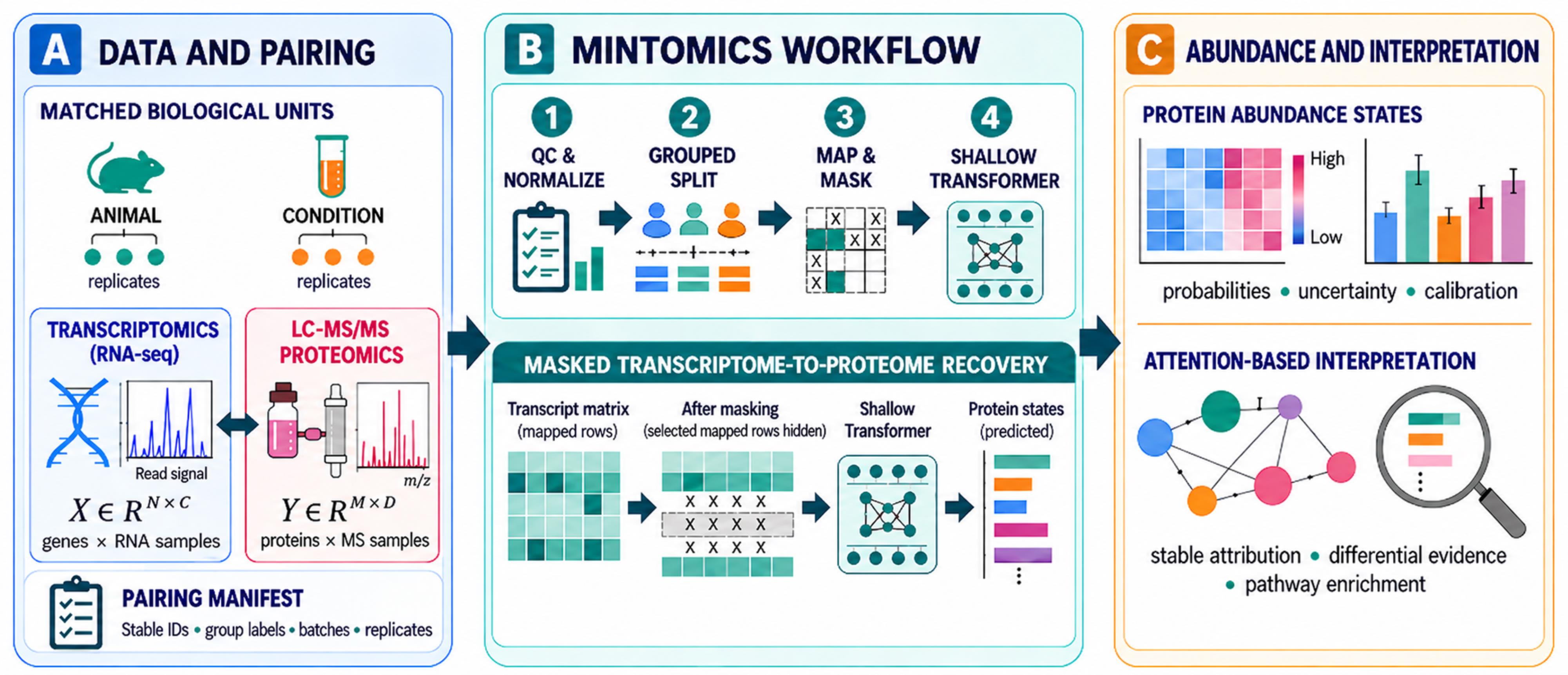
Data requirements, MintOmics workflow, and interpretation. An N × C transcriptomic matrix and an M × D proteomic matrix are connected through P paired biological units and a gene-protein identifier map. Mapped transcript rows are hidden only after biological allocation. The transformer predicts the corresponding protein-abundance states, and the unmasked held-out prediction is integrated with attention, differential expression, differential protein abundance, and pathway enrichment.
Background
Paired transcriptomic and proteomic profiling provides complementary views of biological regulation and can help reveal how gene-expression programs relate to protein abundance across biological conditions [1]. However, RNA and protein abundances are related but non-equivalent measurements because translation efficiency, protein degradation, secretion, post-translational regulation, molecular half-life, and assay-specific measurement processes can produce substantial discordance between the two molecular layers [2]. A further challenge is that these studies may measure thousands of transcripts and proteins while containing only a few biological conditions profiled by both RNA sequencing and mass spectrometry. Consequently, computational models must learn complex cross-omics relationships from a high-dimensional feature space using only a limited number of paired biological states (samples), without any new biological replication.
Several statistical and machine-learning methods have been used to investigate relationships between transcriptomic and proteomic data. Gene-wise correlation and regression analyses can identify direct RNA–protein associations but may not capture nonlinear relationships or contributions from the broader transcriptomic context. Multivariate techniques such as partial least-squares and canonical correlation analysis identify coordinated variation between molecular layers. DIABLO uses supervised latent components for multi-omics integration and biomarker selection [3], whereas multi-omics factor analysis identifies shared and modality-specific sources of variation across omics datasets [4]. These approaches are valuable for dimensionality reduction, sample stratification, and the discovery of molecular signatures; however, their primary purpose is generally to integrate or explain observed molecular layers rather than predict an unmeasured proteomic state from transcriptomic data alone.
Predictive methods have also been developed to infer protein abundance from RNA measurements. For example, cTP-net uses transfer learning to impute cell-surface protein abundance from single-cell transcriptomes [5], and deep neural networks have been applied to predict protein-expression changes from bulk RNA-seq data in large human cohorts [6]. These studies demonstrate that multigene transcriptomic patterns can contain information about protein abundance beyond that provided by the directly corresponding transcript. Nevertheless, their intended applications and data requirements differ from condition-level experiments containing only a few paired biological states. Models trained using large numbers of individuals or cells may not transfer directly to such experiments, and highly parameterized networks are susceptible to overfitting when paired conditions are limited. Furthermore, methods developed for predefined single-cell surface-protein panels do not directly address global LC–MS/MS proteomic measurements from bulk tissues or biological fluids.
MintOmics was developed specifically for this high-dimensional, limited-pairing setting [1]. In the reference mouse oviduct application, bulk RNA-seq and luminal-fluid proteomics were paired across only four biological conditions. Three conditions were used for model development, and the fourth condition was withheld for blind evaluation. The method treats each paired condition as a biological observation and uses computational masking to generate alternative training views of that observation, resulting in a substantial augmentation of training data. These masked views support model optimization but are not considered independent biological samples.
MintOmics formulates transcriptome-to-proteome prediction as a masked gene-to-protein recovery task. Bulk RNA-seq and LC–MS/MS data are filtered and normalized separately, after which gene symbols are linked to protein accessions through an explicit gene-to-protein mapping table. Each gene is represented by its normalized transcriptomic measurements and an optional transcription-factor indicator. During training, selected transcript rows with mapped protein counterparts are masked, and the model is trained to predict the abundance states of the corresponding proteins from the remaining unmasked multigene transcriptomic context. The loss is calculated only for protein positions associated with the transcript rows masked in that training view, thereby preventing genuinely unobserved proteins from being treated as supervised targets.
The reference network uses a shallow transformer encoder based on scaled dot-product self-attention [7]. Self-attention allows the model to represent relationships between a masked transcript and the broader gene-expression profile rather than relying exclusively on the abundance of the directly corresponding transcript. The encoder contains a single attention head, residual connections, layer normalization, and a feed-forward block. Mean pooling and a multilayer perceptron then generate one logit for each mapped protein, representing its predicted relative abundance state. The shallow architecture limits model complexity while retaining the ability to learn multigene relationships in studies with few paired conditions.
Following model development, the selected model is applied to the complete transcriptomic profile of the independently held-out condition. This produces predicted protein-abundance states and a gene-by-gene attention matrix. For biological interpretation, the attention matrix can be restricted to transcription-factor rows and columns associated with mapped proteins. Highly weighted transcription factor–protein combinations can then be integrated with independently calculated differential transcriptomic and proteomic evidence and evaluated using pathway or gene-set enrichment resources. Attention therefore provides a model-derived prioritization score for downstream hypothesis generation.
MintOmics has two principal advantages over methods designed primarily for association analysis or latent-factor integration. First, it performs a directed inference task by predicting relative protein-abundance states from transcriptomic profiles. This is useful when transcriptomic measurements are available more readily than matched proteomic measurements. Second, its attention outputs provide an interpretable representation of the transcriptomic features prioritized during protein-state prediction. These outputs can be combined with differential-expression and pathway evidence to identify candidate regulatory relationships and biological processes for further investigation.
The method also has important limitations. Computational masking increases the number of optimization views but does not create new biological replication or compensate for inadequate biological diversity in the paired conditions. Model performance remains dependent on the number, quality, and representativeness of the conditions used for development. The reference implementation predicts relative binary protein-abundance states rather than absolute or continuous protein concentrations, and prediction is limited to proteins detected by the proteomic assay and represented in the gene-to-protein mapping table. Attention values should not be interpreted as proof of biological causality, and predicted protein states should complement rather than replace direct proteomic measurement.
We envision that the protocol can be applied to developmental stages, disease states, treatment responses, reproductive conditions, genetic perturbations, or other study designs in species other than mice. Application to another organism or experimental system requires an appropriate gene-to-protein mapping resource and, when transcription-factor interpretation is desired, an organism-specific transcription-factor annotation. The framework may also support future extensions to continuous protein-abundance prediction or inference between other paired molecular layers, although these applications would require separate model development, optimization, and validation.
Software and datasets
Run the protocol in an isolated Python environment. Record the exact package versions, operating system, CUDA version, GPU model, source commit, and random seed with the final analysis. The reference MintOmics repository requires Python 3.8 or newer in the commit identifier (shown in Table 1) and the resolved versions of all installed dependencies. It also supplies the processed data, mapping, model, training, inference, and result-analysis scripts [8,9].
Reproducibility note: The validated run used GitHub release (tag: mintomics) Release Mintomicsv1.0 (https://github.com/BioinfoMachineLearning/mintomics/releases/tag/mintomics) with seed 42 on AlmaLinux 8.10 using Python 3.11, PyTorch 2.6.0+cu124, CUDA 12.4, Lightning 2.6.6, NVIDIA driver 570.211.01, and two NVIDIA A100 80 GB PCIe GPUs. The supplied requirements.txt records the Python package environment used for the run. The workflow was validated from a clean clone using the recorded source revision and environment.
License and dependency details:
• PyTorch is distributed under BSD-3-Clause
• Lightning and TorchMetrics under Apache-2.0
• pandas, NumPy, SciPy, mlxtend, and seaborn under BSD-3-Clause
• RNAnorm under Apache-2.0
• Matplotlib uses its PSF-based Matplotlib license
• The Weights & Biases SDK is MIT-licensed (the hosted service is governed separately by its service terms)
• Torch-geometric is MIT-licensed
Table 1. Software, datasets, and validated run environment used in the MintOmics protocol. Exact software versions and hardware correspond to the recorded run environment.
| Type | Software/dataset/resource | Version | Date | License | Access |
|---|---|---|---|---|---|
| Software | MintOmics repository [9] | mintomics (GitHub release tag) | 2025-06-01 | MIT | Free |
| Runtime | Python | 3.11 | Run date | PSF | Free |
| Software | PyTorch, Lightning, torchmetrics [8] | PyTorch 2.6.0+cu124; Lightning 2.6.6; torchmetrics 1.9.0 | Run date | Open source | Free |
| Software | pandas, NumPy, SciPy, rnanorm, mlxtend | pandas 2.3.3; NumPy 2.4.6; SciPy 1.17.1; rnanorm 2.2.0; mlxtend 0.25.0 | Run date | Open source | Free |
| Software | seaborn, matplotlib, Weights & Biases, torch-geometric | seaborn 0.13.2; matplotlib 3.11.2; Weights & Biases 0.30.0; torch-geometric 2.8.0.post1 | Run date | Mixed open source/service | Free tier |
| Data | Processed RNA, protein, mapping, TF, and differential files in Dataset/ | mintomics (GitHub release tag) | 2025-06-01 | Repository license | Free |
| Data | Bulk RNA-seq accession GSE270654 [1] | Deposited study data | 2024 | GEO terms | Free |
| Resource | Reactome 2022 and GO Biological Process 2023 through Enrichr [10,11] | 2022/2023 libraries | Analysis date | Resource dependent | Free |
| Software | Additional active dependencies | PyDESeq2 0.5.4; future 1.0.0; Biopython 1.88; openpyxl 3.1.5 | Run date | Package-specific open-source licenses | Free |
| Runtime | OS/accelerator | AlmaLinux 8.10; CUDA 12.4; NVIDIA driver 570.211.01; 2 x NVIDIA A100 80GB PCIe | Run date | N/A | Institutional hardware |
Additional active dependencies used by the deposited scripts include PyDESeq2 (MIT; Diff_Gene_proc.py), future (MIT; protrank.py), Biopython (Biopython License Agreement, with some BSD-3-Clause components), and an Excel-reading engine such as openpyxl (MIT; genetoprotein.py). Exact package versions, including Lightning, should be taken from and pinned to the validated environment.
Weights & Biases note: Training.py uses WandbLogger for optional experiment logging and accepts user-supplied --entity_name and --project_name values. The workflow can be run with external logging disabled or offline, and the core checkpoints, predictions, and exported analysis files do not depend on the hosted dashboard.
Proteomics data note: The underlying eLife study reports that the proteomic data are available through the oviduct proteomics web-search resource at https://genes.winuthayanon.com/winuthayanon/oviduct_proteins/ (accessed September 20, 2026); the MintOmics protocol itself uses the processed proteomics input distributed for the workflow (Dataset/Labels_orig.csv and the processed files generated from it).
Repository archival note: The repository release is identified by the source release version recorded in Table 1. If a DOI-bearing archive is assigned, cite the archive together with the tested commit or tag.
Transcription-factor annotation source: The mouse transcription-factor (TF) annotation was compiled by integrating unique mouse gene symbols from publicly available resources, including BEELINE (RegNetwork, TRRUST, and ESCAPE) [12], TRRUST v2 [13], AnimalTFDB 4.0 [14], TFcheckpoint 2.0 [15], the cisTarget mouse TF list associated with SCENIC [16], and Mouse Genome Informatics (MGI) annotations for GO:0003700 (DNA-binding transcription factor activity) [17–19]. Duplicate gene symbols were removed to generate a nonredundant mouse TF catalog.
Regarding licensing, TRRUST v2 bulk datasets are distributed under CC BY-SA 4.0, whereas MGI and Gene Ontology annotations are available under CC BY 4.0. The associated publications for AnimalTFDB 4.0 and TFcheckpoint 2.0 are licensed under CC BY 4.0; however, these publication licenses do not necessarily establish separate dataset-level licensing terms. A file-specific license was not identified for the cisTarget mouse TF list.
Procedure
The protocol begins with quantified RNA-seq counts and LC-MS/MS protein abundances. Raw read alignment, peptide identification, and protein inference are outside its scope; those upstream analyses must produce stable gene and protein identifiers and retain sample provenance. MintOmics can be applied to new transcriptomics and proteomics data according to the procedures below.
A. Obtain the software and arrange the paired dataset
1. Clone the MintOmics repository and check out the recorded reference revision. The repository README documents the reference data files, training command, inference command, preprocessing entry point, and output locations.
2. Create a Python 3.11 virtual environment and install the pinned packages from requirements.txt. Save the resolved environment and source revision with each run.
git clone https://github.com/BioinfoMachineLearning/mintomics.gitcd mintomicsgit checkout mintomicspython3.11 -m venv mintomicssource mintomics/bin/activatepython -m pip install -r requirements.txtpython -m pip freeze > software_versions.txt3. Create one row in the pairing table for every biological unit or condition for which both RNA and protein measurements are available, using the required input objects, formats, and dimensions summarized in Table 2. Record the RNA file, protein file, condition, biological source, replicate structure, batch, and analysis role.
Table 2. Required input objects and dimensions. For the reference application, one paired unit is one biological condition; in a new study, use the finest defensible paired biological unit and keep its replicates together.
| Object | Dimensions | Required format | Reference application |
|---|---|---|---|
| Transcriptomics | N × C per paired unit | CSV; first column gene identifier; remaining columns numeric RNA measurements | 21,190 genes × 6 regional replicates |
| TF annotation | N × 1 | One gene symbol per line; capitalization normalized before matching | 1,911 observed |
| Proteomics | M × 1 per paired unit | CSV; Accession column plus one normalized abundance column | 3,060 proteins |
| Gene-protein map | K × 2 | Tab-delimited gene symbol and protein accession without a header | 2,789 records; 2,406 usable pairs |
| Pairing table | P rows | Paired-unit ID, RNA file, protein file, role, biological group | Four condition-level pairs |
4. Pairing-table schema: Create one row for each paired biological unit. The required column names, data types, permitted analysis-role values, and a representative control-condition entry are provided in Supplementary Table S2.1. Supplementary Table S2 separately summarizes the reference biological-condition allocation and corresponding computational-view counts.
5. Assign complete biological groups to training (development) or held-out evaluation before producing masked views. Keep all technical replicates and every later computational view with their source group.
6. For the reference application mentioned, assign control, 0.5 days post coitus (dpc), and 1.5 dpc to development and assign 2.5 dpc to held-out evaluation. For another dataset, replace these labels with study-specific groups without changing the rule that a group occurs in only one role.
7. Place the RNA table at Dataset/Collaboration_data.csv and the protein table at Dataset/Labels_orig.csv. Retain immutable copies of the original files and calculate their SHA-256 hashes.
8. Directory check: Before executing the scripts, ensure that the workflow output directories used by the documented paths exist or are created by the local implementation, including Dataset/Data/, Dataset/Data_cpm/, Dataset/Labels_proc_log10_minmax/, and Dataset/Trainings/<save_dir>
Note: The reference pairing is condition-level rather than specimen-level. Do not manufacture one-to-one pairs between unrelated RNA and proteomic replicates.
B. Preprocess the transcriptomic measurements
1. Read Dataset/Collaboration_data.csv as a tab-delimited matrix with gene identifiers in the first column and RNA samples in the remaining columns.
2. Remove rows with missing gene identifiers. Replace missing count entries with 0 and convert every sample column to numeric values.
3. Calculate the row sum across all RNA samples and retain genes with a total count of at least 10.
4. Select the columns belonging to each paired unit. The reference script uses the patterns control, 0.5preg, 1.5preg, and 2.5preg and retains six columns per condition: three infundibulum-plus-ampulla and three isthmus-plus-uterotubal-junction measurements.
5. Within each selected condition matrix, divide every count by its sample-column total, multiply by 1,000,000 to obtain counts per million (CPM normalization), and apply the inverse hyperbolic sine transformation.
6. Write one processed CSV per paired unit to Dataset/Data_cpm/. Preserve the same gene order in every file.
7. Inspect the processed reference files and confirm that each contains the same set of genes, six measurement columns, finite numeric values, and the same ordered gene identifiers.
8. Reference output filenames are Data_control.csv, Data_0_5preg.csv, Data_1_5preg.csv, and Data_2_5preg.csv. Each file contains the ordered gene identifier followed by six numeric RNA measurement columns. For new datasets, filenames may differ, but the same ordered gene set must be preserved across paired units.
cd Datasetpython ./src/preprocess/Data_preprocessing.pyNote: For a new study, change the sample-selection patterns to the paired-unit labels in the pairing table. Apply the same filtering rule and gene order to every unit.
C. Preprocess the proteomic measurements and create abundance classes
1. Read Dataset/Labels_orig.csv and use the protein accession column as the row identifier.
2. Select the abundance column for each paired unit and remove proteins missing from all selected units.
3. For reproduction of the reference analysis, replace remaining missing abundances with 1 before log10 transformation. In a new experiment, document whether a missing value denotes non-detection, censoring, or a failed measurement before applying an equivalent rule.
4. For each paired unit separately, calculate log10 abundance and min-max scale the resulting protein vector to [0,1]. Save the vector to Dataset/Labels_proc_log10_minmax/ with an Accession column and one numeric abundance column.
5. Create the binary target vector by assigning 1 when the normalized abundance is greater than the selected protein-abundance threshold and 0 otherwise. The reference analysis is repeated with thresholds 0.6 and 0.8; these thresholds define two different target vectors. For advanced analyses, multiple thresholds can be selected to assign more than two classes of abundance.
6. For the reference application, confirm that every reference condition contains 3,060 finite protein values. For 2.5 dpc, the expected positive-class counts are 1,887 at threshold 0.6 and 128 at threshold 0.8.
Critical: The protein-abundance threshold is not the prediction probability cutoff. The former creates the biological target label; the latter converts a model probability to a predicted class.
D. Add transcription-factor annotations and construct the gene-protein map
1. Read the transcription factors (TFs) list (Dataset/Mouse_TFs for reference application) as a one-column list and convert both catalog entries and RNA gene identifiers to uppercase for matching.
2. Create a transcription-factor indicator in the original RNA row order: assign 1 to a gene present in the catalog and 0 otherwise. Append this indicator as the seventh feature column.
3. Implementation check: Verify that the TF flag is generated by testing membership while iterating through the ordered RNA gene list.
4. Input-scaling rule: After RNA preprocessing and TF annotation, clip only the six RNA expression columns at the within-matrix 99.9th percentile and divide those six columns by that percentile. Keep the TF indicator as a binary 0/1 feature. Apply the same expression-scaling rule to development, validation, held-out diagnostic, and blind-inference matrices.
5. Save the two-column gene-symbol-to-protein-accession mapping as Dataset/genetoprotein.csv using tab delimiters and no header. The processed RNA and protein inputs resolve from Dataset/Data_cpm/ and Dataset/Labels_proc_log10_minmax/, respectively.
6. The finalized loaders use Dataset/genetoprotein.csv as the canonical mapping path and report 2,789 mapping rows, 2,671 genes represented in the map, and 2,406 retained gene-protein pairs for model evaluation. For a new organism, supply an externally generated organism-appropriate two-column gene-symbol/protein-accession mapping.
7. Create a gene dictionary from the processed RNA row order and a protein dictionary from the processed proteomics row order.
8. Retain mapping records whose gene occurs in the gene dictionary and whose protein occurs in the protein dictionary. Convert every retained pair to a zero-based gene index and protein index.
9. For the reference dataset, confirm 2,789 mapping records, 2,671 mapped genes in the RNA matrix, 2,515 mapped proteins in the protein matrix, and 2,406 jointly usable index pairs.
Note: There is no universal minimum acceptable mapping percentage for a new dataset. Report the fractions of RNA genes and proteomic targets retained after mapping, resolve identifier namespace, capitalization, species, and database-version mismatches, and interpret downstream results cautiously when the retained mapped set is small or unrepresentative of the intended protein targets.
Critical: Construct the TF indicator from the ordered gene list, not by iterating through a set; otherwise, the annotation can be assigned to the wrong rows.
E. Generate independent mapped masking views
1. Set the random seed to 42 before generating random views. Keep separate random-number streams or saved index files for training, validation, and held-out diagnostic views.
2. For every view, start from an unmodified copy of the condition matrix before rows are zeroed. The finalized loaders implement this with np.array(dat, copy=True) before masking in the training, held-out, and differential loaders, preventing masks from accumulating across successive views.
3. Randomly sample mapped gene indices without replacement. In the reference dataset, 400 corresponds to 15% of the 2,671 mapped gene symbols present in the RNA matrix, calculated as [2,671 × 0.15].
4. Set all seven feature values of the selected gene rows to 0.
5. Translate the selected gene indices to their paired protein indices using the ordered gene-protein map. Store the result as a 2 × 400 integer array in which the first row contains gene indices and the second row contains protein indices.
6. Attach the complete 3,060-position binary protein target vector to the view. During training, index this vector only at the 400 mapped protein positions.
7. Generate 4,000 training views and 1,000 validation views for each of the three development conditions in the reference reproduction, yielding 12,000 training and 3,000 validation views. Generate 2,000 masked 2.5 dpc views only as a held-out recovery diagnostic. This random masking technique can effectively generate a large amount of data (views) from a small number of paired samples to train and test the transformer model, which is one key innovation in MintOmics.
8. For final blind inference, create one 2.5 dpc view with no masked rows and an index array containing all 2,406 jointly usable pairs.
9. View generation, storage, and verification:
a. The reference MintOmics implementation generates masked computational views directly in memory; individual views and index arrays are not written to disk by default. Consequently, there is no mandatory file format, naming convention, or storage directory for this step.
b. To verify successful generation, confirm that the reference dataset produces 12,000 training views, 3,000 validation views, and 2,000 masked held-out diagnostic views. Each view contains an input matrix of dimensions 21,190 × 7, a binary protein target vector of length 3,060, and a 2 × 400 integer index array. The first row of the index array contains the selected gene indices, and the second row contains their corresponding protein indices. Confirm that exactly 400 mapped transcript rows are masked per view and that every view is generated from a fresh copy of the original condition matrix to prevent cumulative masking.
c. For users requiring persistent records, individual views may optionally be serialized as NumPy archives (.npz) containing the input matrix, protein target vector, and gene–protein index array. The source biological condition, analysis partition, random seed, masking fraction, and view identifier should also be recorded. Such serialization is optional and is not performed automatically by the reference loader.
Critical: A generated view is not a biological replicate. Report three development conditions and one held-out condition for the reference study, not 17,000 samples.
Data analysis
A. Build the MintOmics transformer
1. Set the input dimension F to the number of RNA and annotation features per gene, the sequence length N to the number of retained genes, and the output dimension M to the number of proteins. The reference values are F = 7, N = 21,190, and M = 3,060.
2. Create one batch-first transformer encoder layer with model dimension 7, one attention head, feed-forward dimension 32, dropout 0.5, residual connections, and layer normalization (Figure 1).
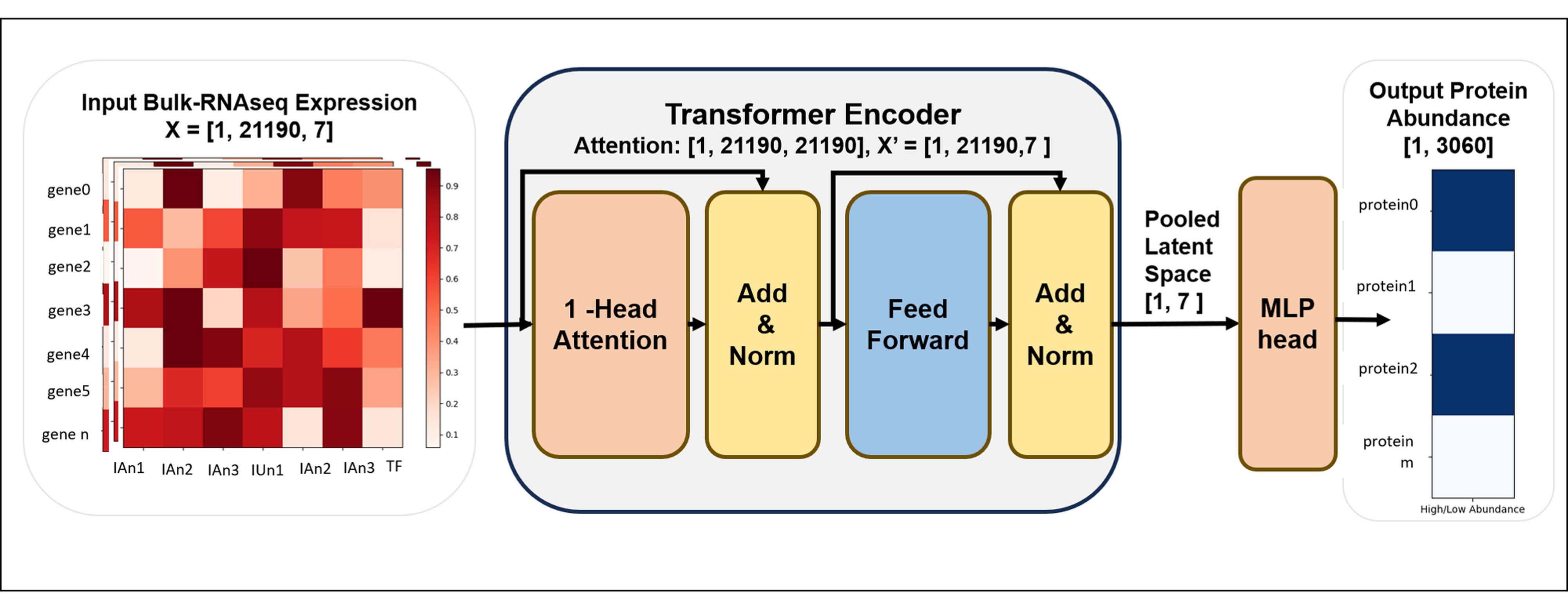
Figure 1. MintOmics transformer architecture for the referenced application. Each gene is a seven-dimensional token comprising six RNA-seq measurements and one transcription-factor indicator. A single-head self-attention encoder contextualizes the genes. Mean pooling and the multilayer-perceptron head produce one protein-abundance logit for every protein target. Tensor dimensions are B × N × 7 at the encoder input, B × N × N for the averaged attention matrix, B × 7 after mean pooling, and B × M for the protein-output logits (B × 3,060 in the reference application). For batch size 1 in the reference dataset, the encoder input is (1, 21190, 7), the attention matrix is (1, 21190, 21190), the pooled representation is (1, 7), and the protein-output logits are (1, 3060).
3. Apply the encoder to a tensor of shape B × N × 7 and retain both the contextualized tensor and the averaged attention matrix of shape B × N × N.
4. Mean-pool the contextualized tensor across the N genes to obtain B × 7 and apply the ReLU activation function.
5. Pass this representation through a multi-layer perceptron (MLP) containing two ReLU-activated hidden layers of 896 and 224 units, corresponding to 128 and 32 times the seven-dimensional model representation, respectively. Project the final hidden representation to 3,060 output logits, one for each protein in the ordered reference proteomic vector. These hidden-layer widths are hyperparameters of the reference implementation; the deposited code does not report a separate optimization or ablation analysis supporting their selection.
6. Return raw logits; do not apply sigmoid inside the model.
7. For a masked batch, gather the 400 output logits at the mapped protein indices and compute BCEWithLogitsLoss against the corresponding binary targets.
8. (Critical) Before training, verify the tensor dimensions and identifier order: input B × N × 7, attention B × N × N, pooled representation B × 7, output B × M, and masked index 2 × K (2 × 400 in the reference masked views). Confirm that the gene and protein dictionaries used to construct the index are the same dictionaries used by the model inputs and targets.
B. Configure and train the reference model
1. In Training.py, set Num_classes to M, ATT_HEAD to 1, ENCODE_LAYERS to 1, BATCH_SIZE to 1, and the data-view calls to 4,000 training, 1,000 validation, and 2,000 held-out diagnostic views with pertage = 0.15, where pertage denotes the masking fraction.
2. Implementation note: --batch_size now controls the DataLoader directly. The reference value is 1, and the same value is used in the documented training command.
3. Initialize Python, NumPy, and PyTorch through pl.seed_everything(42). Enable deterministic cuDNN execution and disable cuDNN benchmarking.
4. Use Adam with a learning rate of 0.0001 and BCEWithLogitsLoss on the mapped protein positions.
5. Reduce the learning rate by a factor of 0.1 after 20 epochs without improvement in validation loss, with epsilon 1 × 10⁻¹⁰.
6. Train for at most 100 epochs. Stop after 30 epochs without validation-loss improvement and retain the 10 checkpoints with the lowest validation loss.
7. Shuffle the training loader and keep validation and held-out loaders ordered. Use one data-loader worker in the reference reproduction.
8. Run the training command from Dataset/ so that the data paths used by the loaders resolve correctly. Select the checkpoint with the lowest validation loss.
cd DatasetPYTHONPATH=..:../src/model:../src/dataset python ../Training.py \ --num_gpus 1 --nodes 1 --num_epochs 100 \ --batch_size 1 --abundance_threshold 0.6 --save_dir reference_run# repeat as a separate run with --abundance_threshold 0.89. Weights & Biases execution note: Experiment logging is optional. When online logging is used, supply --entity_name and --project_name values for the user's own account/project. The workflow can also be run with external logging disabled or offline; core prediction and checkpoint outputs are independent of the hosted dashboard.
10. Expected successful-run outputs: Checkpoints are written under Trainings/<save_dir>
Expected result for reference application: The loader reports tensors of 12,000 × 21,190 × 7 for training, 3,000 × 21,190 × 7 for validation, and 2,000 × 21,190 × 7 for the masked held-out diagnostic. The corresponding protein target dimension is 3,060, and the masked index dimension is 2 × 400 per view.
C. Run blind inference and calculate protein-abundance metrics
1. Set the held-out loader to size = 1 and pertage = 0 so that no gene rows are removed, and all usable gene-protein pairs (e.g., 2,406 in the reference application) are evaluated.
2. Load the checkpoint selected by development validation loss. Set the model to evaluation mode and disable gradient calculation.
3. Pass the complete held-out RNA matrix through the model and gather logits at the mapped protein indices (e.g., 2,406 indices in the reference application).
4. Apply the sigmoid function to obtain protein-abundance probabilities and apply a probability cutoff (e.g., 0.5 in the reference application) to create predicted classes.
5. Join every probability and predicted class to the protein accession, mapped gene identifier, observed abundance class, target-abundance threshold, condition, seed, and checkpoint.
6. Calculate accuracy, precision, recall, and F1 across the mapped proteins. Repeat the complete target-generation, training, and inference sequence separately for target thresholds (e.g., 0.6 and 0.8 in the reference application).
7. The current training and held-out inference interfaces expose --abundance_threshold (default 0.8). For reproducibility, pass the intended threshold explicitly and run target generation, training, and inference separately at 0.6 and 0.8. Do not derive one threshold result by relabeling predictions from a model trained at the other threshold.
8. Export the long-form prediction table and the 2 × 2 confusion matrix before producing plots.
cd DatasetPYTHONPATH=..:../src/model:../src/dataset python ../Inference.py \ --save_dir reference_run --chkpt mintomics_best.ckpt --abundance_threshold 0.6Note: Replace mintomics_best.ckpt with the filename of the checkpoint selected by validation loss. The protein target threshold and the probability cutoff threshold answer different questions and must be reported separately.
D. Extract and summarize attention
1. Obtain the N × N self-attention matrix returned by the unmasked held-out inference pass. This can be analyzed for any unmasked biological conditions.
2. Set its diagonal to 0 so that self-attention does not dominate the ranking.
3. Select the columns corresponding to the mapped gene indices and label each selected column with its paired protein accession.
4. Retain proteins that meet the selected high-abundance target definition or the prespecified influential-protein rule.
5. Select rows whose TF indicator equals 1 and label them with the ordered RNA gene symbols.
6. For each retained protein, rank TF rows by attention score and keep the top TFs (e.g., top 25 in the reference application) for reproduction of the reported downstream analysis.
7. Export a long-form table containing condition, protein accession, TF gene symbol, raw attention score, rank, target threshold, and checkpoint.
E. Integrate attention with differential and pathway evidence
1. Prepare differential gene-expression tables for the selected biological contrasts using the original RNA biological replicates, not the masked views.
2. Required differential-analysis fields: The gene-expression table should contain a gene identifier, effect-size field (for example, log2 fold change), adjusted P value, and significance designation; the protein-abundance table should contain a protein accession, effect-size field, adjusted P value, and significance designation. Use the same biological contrast labels in both tables.
3. Prepare differential protein-abundance tables for the same contrasts using the original proteomic biological units.
4. Map significant protein accessions to their corresponding genes and retain proteins supported by both differential layers. Record the effect direction and significance criteria used in each layer (Figure 2).
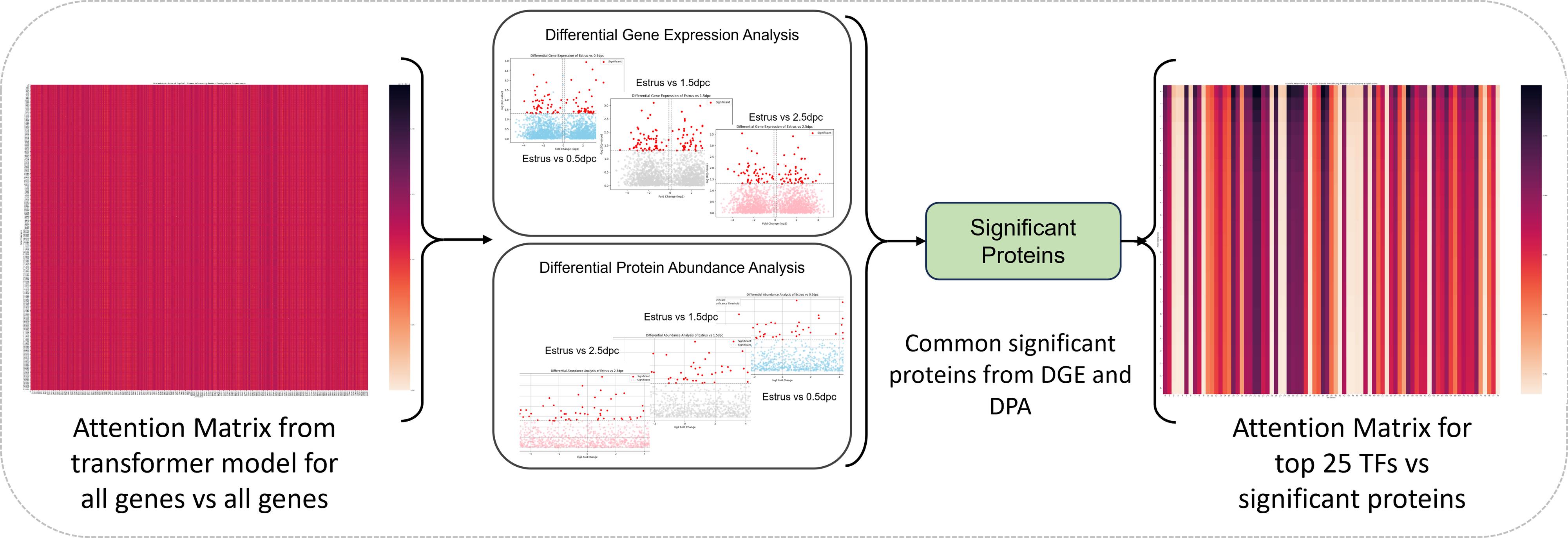
Figure 2. Downstream attention and evidence-integration analysis. The gene-by-gene attention matrix is combined with differential gene-expression and differential protein-abundance results. Proteins significant in both measured layers define the influential-protein set, and the top transcription factors (e.g., top 25 in the reference application) by attention are retained for each selected protein before pathway analysis.
5. Clarification: MintOmics compares differential gene-expression evidence with differential protein-abundance evidence after protein-level quantification and gene-protein mapping (Figure 2). It does not perform a direct differential gene vs. differential peptide comparison. Peptide identification and peptide-to-protein inference are upstream analyses outside the scope of this protocol.
6. Join the influential-protein set to the exported attention table for top TFs (e.g., top 25 in the reference application).
7. For the reference analysis, prepare combined TF and influential-protein lists for estrus (control) vs. 0.5 dpc, estrus vs. 1.5 dpc, and estrus vs. 2.5 dpc.
8. Submit each list to Enrichr and select Reactome 2022 and GO Biological Process 2023 [10,11]. Download the complete enrichment tables, not only the significant rows.
9. Report the input list, background universe when specified, library name and version, adjusted P value, overlap genes, and analysis date.
Generation of intermediate analysis files: The reference intermediate files are generated by the attention and differential-expression analyses. Inference.py (--timepoint all) processes the unmasked 21,190 × 21,190 attention matrix by removing diagonal values and retaining columns corresponding to the 2,406 mapped gene–protein pairs. The top 25 ranked TFs and their transformed attention scores [sigmoid(attention × 10,000)] are exported as Tfs_allprot_<condition>
Separately, src/preprocess/Diff_Gene_proc.py performs PyDESeq2 comparisons of 0.5, 1.5, and 2.5 dpc against Finnerty control (TC). Genes satisfying padj < 0.05 and |log2FoldChange| > 0.1 and mapping to measured proteins are exported as Siggenebasedprotlist_TCT<condition>
These intermediate files are integrated using:
cd DatasetPYTHONPATH=..:../src/model:../src/dataset python ../Result_analysis.pyThe script generates four contrast-specific AllTfs_diffcodinggene_<condition>.csv outputs (control, 0_5, 1_5, and 2_5). Functional enrichment is performed separately using Enrichr. Intermediate filenames may vary for other datasets. Note: Attention ranks model associations; it does not establish transcription-factor regulation. Interpret a TF–protein pair as a hypothesis supported by the model and the stated orthogonal evidence.
Result interpretation
In the reference analysis, each processed RNA matrix contains 21,190 genes, each proteomic vector contains 3,060 proteins, the identifier map yields 2,406 jointly usable gene–protein pairs, each masked view removes 400 mapped genes, and 1,911 transcription factors are represented in the RNA input. Different datasets may yield different dimensions; record those dimensions and preserve identifier order through training and inference.
As shown in Table 3, at threshold 0.6 for protein concentration, the reported model retains high precision while recovering most high-abundance targets. At threshold 0.8, accuracy increases because the positive class is smaller, whereas recall and F1 decrease. These values demonstrate the sensitivity of performance to the biological target definition and should not be interpreted as interchangeable confidence thresholds. Supplementary Figure S3 provides the held-out threshold 0.6 prediction diagnostic, including the probability distributions and mapped-pair confusion matrix (TN = 860, FP = 18, FN = 205, TP = 1,323).
For a new study, interpret performance relative to class prevalence and the held-out biological group. A single held-out condition demonstrates transfer to that condition within the measured system; it does not establish cross-population, cross-species, or cross-laboratory generalization.
Table 3. Representative blind-test performance reported for the 2.5 dpc condition [1]. The two rows use different normalized protein-abundance thresholds to create the target labels; both use a prediction probability cutoff of 0.5.
| Target-abundance threshold | Accuracy | F1 | Precision | Recall |
|---|---|---|---|---|
| 0.6 | 0.907 | 0.922 | 0.986 | 0.866 |
| 0.8 | 0.983 | 0.778 | 0.972 | 0.648 |
Validation of protocol
This protocol was used and validated in the following research article:
• Finnerty et al. [1]. Multi-omics analyses and machine learning prediction of oviductal responses in the presence of gametes and embryos, eLife (Figure 4 and Figure 4, figure supplement 1B).
The study trained the transformer with control, 0.5 dpc, and 1.5 dpc data and blindly evaluated the 2.5 dpc condition. The same work integrated attention-ranked transcription factors with differential transcriptomic and proteomic evidence.
General notes and troubleshooting
General notes
1. Treat paired biological conditions, animals, donors, or samples as independent units. Masks and repeated optimization views do not change the biological sample size.
2. Keep gene order, protein order, TF indicators, and gene–protein index pairs fixed after construction. Save the dictionaries beside each checkpoint.
3. Use a fresh expression-matrix copy for every mask. Accumulating zeros across successive views changes the training task. The implementation creates every masked view from np.array(dat, copy=True) before zeroing selected rows.
4. The reference target is relative abundance within a condition after min-max scaling; it is not an absolute protein concentration.
5. Full attention over N genes requires memory proportional to N squared. Batch size one is used in the reference workflow. The validated run used NVIDIA A100 80GB PCIe hardware; a measured held-out forward pass peaked at approximately 4.06 GB GPU memory. This measured value is hardware- and implementation-specific rather than a universal minimum.
6. Repeat the entire training sequence when the protein target threshold changes; do not relabel predictions from a model trained on another target vector.
7. For downstream differential analyses, biological replicates or independent biological units define the inferential sample size. Technical replicates and repeated computational masking views are not independent. If technical replicates are present, document their upstream handling or aggregation before MintOmics integration.
8. Before training a new dataset, verify the number of independent paired biological units, group-exclusive partitioning, the number and fraction of mapped gene–protein pairs, positive-class count and prevalence at the selected target threshold, fixed identifier order, and available memory for the N × N attention matrix. In the reference analysis, positive-class counts at threshold 0.6 were 1,523, 1,696, and 1,719 across the three development stages and 1,887 in the held-out stage; at threshold 0.8, the corresponding counts were 84, 93, 96, and 128.
9. Record the elapsed runtime and approximate storage used for preprocessing, optional view serialization, training, checkpoint retention, blind inference, and attention export on the stated hardware. Runtime and storage are implementation- and hardware-dependent. On the reported A100 hardware, a measured training epoch required approximately 31 min at roughly 6 iterations/s. Dataset/ occupied approximately 24 MB when measured, with additional storage used by checkpoints under Trainings/.
10. Statsmodels and rpy2 are not included as runtime dependencies because the corresponding alternative code is contained in a non-executed triple-quoted block.
Troubleshooting
Problem 1: The preprocessing script cannot find an input file.
Possible cause: The command was run from the repository root although the script uses paths relative to Dataset/.
Solution: Change to Dataset/ before running the preprocessing, training, inference, or result-analysis command shown in this protocol.
Problem 2: The mapping step returns fewer usable pairs than expected.
Possible cause: Gene symbols and protein accessions use different capitalization, namespaces, or row identifiers.
Solution: Normalize gene capitalization, verify the protein Accession column, confirm the tab-delimited mapping file, and rebuild both ordered dictionaries. Report the mapping fractions for RNA genes and protein targets; if mapping is substantially lower than expected, resolve identifier/species/version mismatches before continuing and assess whether the retained targets remain representative.
Problem 3: The TF count is correct, but TF labels appear on the wrong genes.
Possible cause: The indicator was created by iterating over an unordered set.
Solution: Create the indicator by iterating through the original RNA gene list and testing membership in the TF catalog.
Problem 4: Later masked views contain almost no mapped transcript signal.
Possible cause: The same expression array was modified repeatedly, so masking accumulated across views.
Solution: Copy the complete condition matrix before applying every independently sampled mask.
Problem 5: Training or inference exhausts GPU memory.
Possible cause: The returned N × N attention matrix is large, and self-attention scales quadratically with the gene count.
Solution: Use batch size one, close other GPU processes, and record any feature-reduction modification as a new validated analysis. Record the GPU model and memory used for the run. Because the required memory depends on N and the implementation, do not treat a single memory value as a universal minimum.
Problem 6: Inference produces nearly one class only.
Possible cause: The target-abundance threshold produces a highly imbalanced target, or the wrong cutoff was applied to logits.
Solution: Inspect the positive-class count, convert logits with sigmoid, apply the 0.5 probability cutoff, and report precision, recall, and F1 with accuracy. Report class prevalence for every target threshold and interpret precision, recall, and F1 alongside accuracy. If reweighting or resampling is introduced for a new dataset, document and validate it as a modified analysis.
Problem 7: Result_analysis.py cannot locate an intermediate CSV.
Possible cause: The attention and differential-analysis tables were not exported with the filenames expected by the application-specific script.
Solution: Export the TF-by-protein attention table and the contrast-specific differential gene/protein lists first, then update the filenames in Result_analysis.py to the recorded condition labels. In the deposited Result_analysis.py workflow, examples include Data/Diff_data/diff_ctr_TC.csv, Data/Diff_labels/luminal protein estrus.csv, Tfs_allprot_<condition>
Supplementary information
The following supporting information can be downloaded here:
1. Table S1. Reference input files and expected dimensions.
2. Table S2. Reference pairing, development, validation, and held-out allocation.
3. Table S3. Reference identifier, mapping, and masking values.
4. Table S4. Reference architecture and training parameters.
5. Figure S1. Representative masking schematic and masking_example.csv showing mapped transcript rows before and after masking with corresponding protein indices.
6. Figure S2. Representative training and validation loss and metric curves for the TF-ordered 0.6 analysis.
7. Figure S3. Held-out predicted vs. true protein-abundance diagnostic, including probability distributions and the mapped-pair confusion matrix.
8. Figure S4. Representative TF-protein attention heatmap and ranked transcription-factor output.
9. Figure S5. Representative pathway-enrichment output generated from the supplied combined TF and influenced-protein Enrichr workbooks.
10. Table S5. Representative 2.5 dpc prediction metrics.
11. Table S6. Required prediction, attention, differential, and enrichment output fields.
Acknowledgments
This protocol was developed from the MintOmics analysis reported by Finnerty et al. [1].
The underlying study was supported by NSF CCF2343612, NSF IOS2525780, NIH R01HD097087, NIH R21HD119276, NIH R03HD121464, NIH T32GM008336, a University of Missouri start-up fund, and a Washington State University Office of Research RA + $10K award. The funders had no role in study design, data collection and interpretation, or the decision to submit the work for publication.
Author contributions
Conceptualization, J.C., A.H., and W.W.; Data collections and curation, A.H., Y.W., R.M.F., S.W.; Software, A.H., Y.W., and F.B.; Formal analysis, A.H.; Validation, A.H.; Visualization, A.H.; Methodology, A.H., J.C., and W.W.; Writing—original draft, A.H.; Writing—review and editing, A.H., Y.W., F.B., J.C., and W.W.; Resources, J.C. and W.W.; Supervision, J.C. and W.W.; Project administration, J.C., W.W., and A.H.; Funding acquisition, J.C. and W.W.
Competing interests
The authors declare no conflicts of interest.
Ethical considerations
The computational protocol introduces no new animal experiments. The mouse data used to validate MintOmics were generated under Washington State University and University of Missouri Animal Care and Use Committee approvals 6147, 6151, 38927, and 38961, and the study followed ARRIVE guidelines [1].
References
- Finnerty, R. M., Carulli, D. J., Hedge, A., Wang, Y., Boadu, F., Winuthayanon, S., Jack Cheng, J. and Winuthayanon, W. (2025). Multi-omics analyses and machine learning prediction of oviductal responses in the presence of gametes and embryos. eLife. 13: e100705. https://doi.org/10.7554/elife.100705
- Vogel, C. and Marcotte, E. M. (2012). Insights into the regulation of protein abundance from proteomic and transcriptomic analyses. Nat Rev Genet. 13(4): 227–232. https://doi.org/10.1038/nrg3185
- Singh, A., Shannon, C. P., Gautier, B., Rohart, F., Vacher, M., Tebbutt, S. J. and Lê Cao, K. A. (2019). DIABLO: an integrative approach for identifying key molecular drivers from multi-omics assays. Bioinformatics. 35(17): 3055–3062. https://doi.org/10.1093/bioinformatics/bty1054
- Argelaguet, R., Velten, B., Arnol, D., Dietrich, S., Zenz, T., Marioni, J. C., Buettner, F., Huber, W. and Stegle, O. (2018). Multi‐Omics Factor Analysis—a framework for unsupervised integration of multi‐omics data sets. Mol Syst Biol. 14(6): e20178124. https://doi.org/10.15252/msb.20178124
- Zhou, Z., Ye, C., Wang, J. and Zhang, N. R. (2020). Surface protein imputation from single cell transcriptomes by deep neural networks. Nat Commun. 11(1): 651. https://doi.org/10.1038/s41467-020-14391-0
- Tasaki, S., Xu, J., Avey, D. R., Johnson, L., Petyuk, V. A., Dawe, R. J., Bennett, D. A., Wang, Y. and Gaiteri, C. (2022). Inferring protein expression changes from mRNA in Alzheimer’s dementia using deep neural networks. Nat Commun. 13(1): 655. https://doi.org/10.1038/s41467-022-28280-1
- Vaswani, A., Shazeer, N., Parmar, N., Uszkoreit, J., Jones, L., Gomez, A. N., Kaiser, L. and Polosukhin, I. (2017). Attention is all you need. Advances in Neural Information Processing Systems. 30.
- Paszke, A., Gross, S., Massa, F., Lerer, A., Bradbury, J., Chanan, G., Killeen, T., Lin, Z., Gimelshein, N., Antiga, L., et al. (2019). PyTorch: an imperative style, high-performance deep learning library. Advances in Neural Information Processing Systems. 32: 8024–8035.
- BioinfoMachineLearning. MintOmics: Integration of Transcriptomics to Proteomics using Transformer. GitHub release, tag: mintomics. https://github.com/BioinfoMachineLearning/mintomics/releases/tag/mintomics (accessed October 2, 2026).
- Chen, E. Y., Tan, C. M., Kou, Y., Duan, Q., Wang, Z., Meirelles, G. V., Clark, N. R. and Ma’ayan, A. (2013). Enrichr: interactive and collaborative HTML5 gene list enrichment analysis tool. BMC Bioinf. 14(1): 128. https://doi.org/10.1186/1471-2105-14-128
- Kuleshov, M. V., Jones, M. R., Rouillard, A. D., Fernandez, N. F., Duan, Q., Wang, Z., Koplev, S., Jenkins, S. L., Jagodnik, K. M., Lachmann, A., et al. (2016). Enrichr: a comprehensive gene set enrichment analysis web server 2016 update. Nucleic Acids Res. 44: W90–W97. https://doi.org/10.1093/nar/gkw377
- Pratapa, A., Jalihal, A. P., Law, J. N., Bharadwaj, A. and Murali, T. M. (2020). Benchmarking algorithms for gene regulatory network inference from single-cell transcriptomic data. Nat Methods. 17(2): 147–154. https://doi.org/10.1038/s41592-019-0690-6
- Han, H., Cho, J. W., Lee, S., Yun, A., Kim, H., Bae, D., Yang, S., Kim, C. Y., Lee, M., Kim, E., et al. (2017). TRRUST v2: an expanded reference database of human and mouse transcriptional regulatory interactions. Nucleic Acids Res. 46: D380–D386. https://doi.org/10.1093/nar/gkx1013
- Shen, W. K., Chen, S. Y., Gan, Z. Q., Zhang, Y. Z., Yue, T., Chen, M. M., Xue, Y., Hu, H. and Guo, A. Y. (2022). AnimalTFDB 4.0: a comprehensive animal transcription factor database updated with variation and expression annotations. Nucleic Acids Res. 51: D39–D45. https://doi.org/10.1093/nar/gkac907
- Acencio, M. L., Vazquez, M., Chawla, K., Lægreid, A. and Kuiper, M. (2023). TFCheckpoint database update, a cross-referencing system for transcription factors from human, mouse and rat. Nucleic Acids Res. 52: D334–D344. https://doi.org/10.1093/nar/gkad1030
- Aibar, S., González-Blas, C. B., Moerman, T., Huynh-Thu, V. A., Imrichova, H., Hulselmans, G., Rambow, F., Marine, J. C., Geurts, P., Aerts, J., et al. (2017). SCENIC: single-cell regulatory network inference and clustering. Nat Methods. 14(11): 1083–1086. https://doi.org/10.1038/nmeth.4463
- Baldarelli, R. M., Smith, C. L., Ringwald, M., Richardson, J. E., Bult, C. J., Anagnostopoulos, A., Begley, D. A., Bello, S. M., Christie, K., Finger, J. H., et al. (2024). Mouse Genome Informatics: an integrated knowledgebase system for the laboratory mouse. Genetics. 227(1): e1093/genetics/iyae031. https://doi.org/10.1093/genetics/iyae031
- Ashburner, M., Ball, C. A., Blake, J. A., Botstein, D., Butler, H., Cherry, J. M., Davis, A. P., Dolinski, K., Dwight, S. S., Eppig, J. T., et al. (2000). Gene Ontology: tool for the unification of biology. Nat Genet. 25(1): 25–29. https://doi.org/10.1038/75556
- The Gene Ontology Consortium. (2026). The Gene Ontology knowledgebase in 2026. Nucleic Acids Res. 54: D1779–D1792. https://doi.org/10.1093/nar/gkaf1292
Article Information
Publication history
Received: Aug 26, 2026
Accepted: Oct 14, 2026
Available online: Nov 2, 2026
Published: Nov 20, 2026
Copyright
© 2026 The Author(s); This is an open access article under the CC BY license (https://creativecommons.org/licenses/by/4.0/).
How to cite
Readers should cite both the Bio-protocol article and the original research article where this protocol was used:
- Hegde, A., Wang, Y., Boadu, F., Finnerty, R. M., Winuthayanon, W. and Cheng, J. (2026). Predicting Proteomics Data From Transcriptomics Data With MintOmics. Bio-protocol 16(22): e5873. DOI: 10.21769/BioProtoc.5873.
- Finnerty, R. M., Carulli, D. J., Hedge, A., Wang, Y., Boadu, F., Winuthayanon, S., Jack Cheng, J. and Winuthayanon, W. (2025). Multi-omics analyses and machine learning prediction of oviductal responses in the presence of gametes and embryos. eLife. 13: e100705. https://doi.org/10.7554/elife.100705

 Download Citation in RIS Format
Do you have any questions about this protocol?
Post your question to gather feedback from the community. We will also invite the authors of this article to respond.
 Post a Question


