


- Protocols

- Articles and Issues
- For Authors
- About
- Become a Reviewer


Semi-Automated Workflow for Segmenting and Quantifying Ribosomes in Electron Tomograms of High-Pressure Frozen and Resin-Embedded Samples

(*contributed equally to this work) Published: Vol 16, Iss 22, Nov 20, 2026 DOI: 10.21769/BioProtoc.5866 Views: 44
Reviewed by: Matthew RussellElena A. OstrakhovitchAnonymous reviewer(s)
 PDF
 Ask a question

Original research article
The authors used this protocol in:

Sep 2025

Protocol Collections
Comprehensive collections of detailed, peer-reviewed protocols focusing on specific topics



Abstract
Ribosomes are the central molecular machines of protein synthesis, and accurate counts of ribosome numbers are essential for linking translational capacity to cellular physiology. Common approaches infer ribosome abundance indirectly, for example, by measuring rRNA or ribosomal proteins, which can obscure spatial heterogeneity and sample-specific differences. This protocol presents an accessible image analysis pipeline for segmenting and counting individual ribosomes in three-dimensional transmission electron microscopy (3D-TEM) data. Established experimental procedures, namely high-pressure freezing (HPF), freeze substitution, resin embedding, serial semi-thick sectioning, and dual-axis tomography, are summarized here with direct references to primary protocols. The core of this work details electron tomography reconstruction and dual-axis stitching in IMOD 5.1, region-of-interest cropping in Fiji, and a semi-automated segmentation pipeline in arivis Pro 4.5. This pipeline inverts and denoises tomograms, detects ribosomal particles with a tuned Blob Finder routine, applies empirically derived voxel-count thresholds alongside a laboratory-specific shrinkage correction, and converts segmented counts to ribosomes per cubic micrometer and, for cultured cells, per cell. Validation shows that tomographic counts agree with independent biochemical rRNA measurements to within the same order of magnitude, and the protocol states the false-positive and false-negative limitations inherent to nonspecific heavy-metal staining.
Key features
• Detailed image analysis pipeline for ribosome segmentation in electron tomograms using IMOD, Fiji, and arivis Pro, with recommended parameter values.
• Condensed but executable sample-preparation section covering high-pressure freezing, freeze substitution, resin embedding, sectioning, and dual-axis tomography for both C. elegans and cultured mammalian (hTERT-RPE-1) cells.
• Shrinkage-corrected quantification that converts voxel counts to ribosomes per cubic micrometer and per cell using an empirically derived shrinkage factor of 1.575.
• Validation of ribosome counts at 25, 50, and 100 voxel thresholds in control and rpoa-1(RNAi) samples using an independent biochemical method.
Keywords: Ribosome quantification Electron tomography
High-pressure freezing
Freeze-substitution
arivis Pro
IMOD
image segmentation
Shrinkage correction
hTERT-RPE-1
C. elegans
Graphical overview
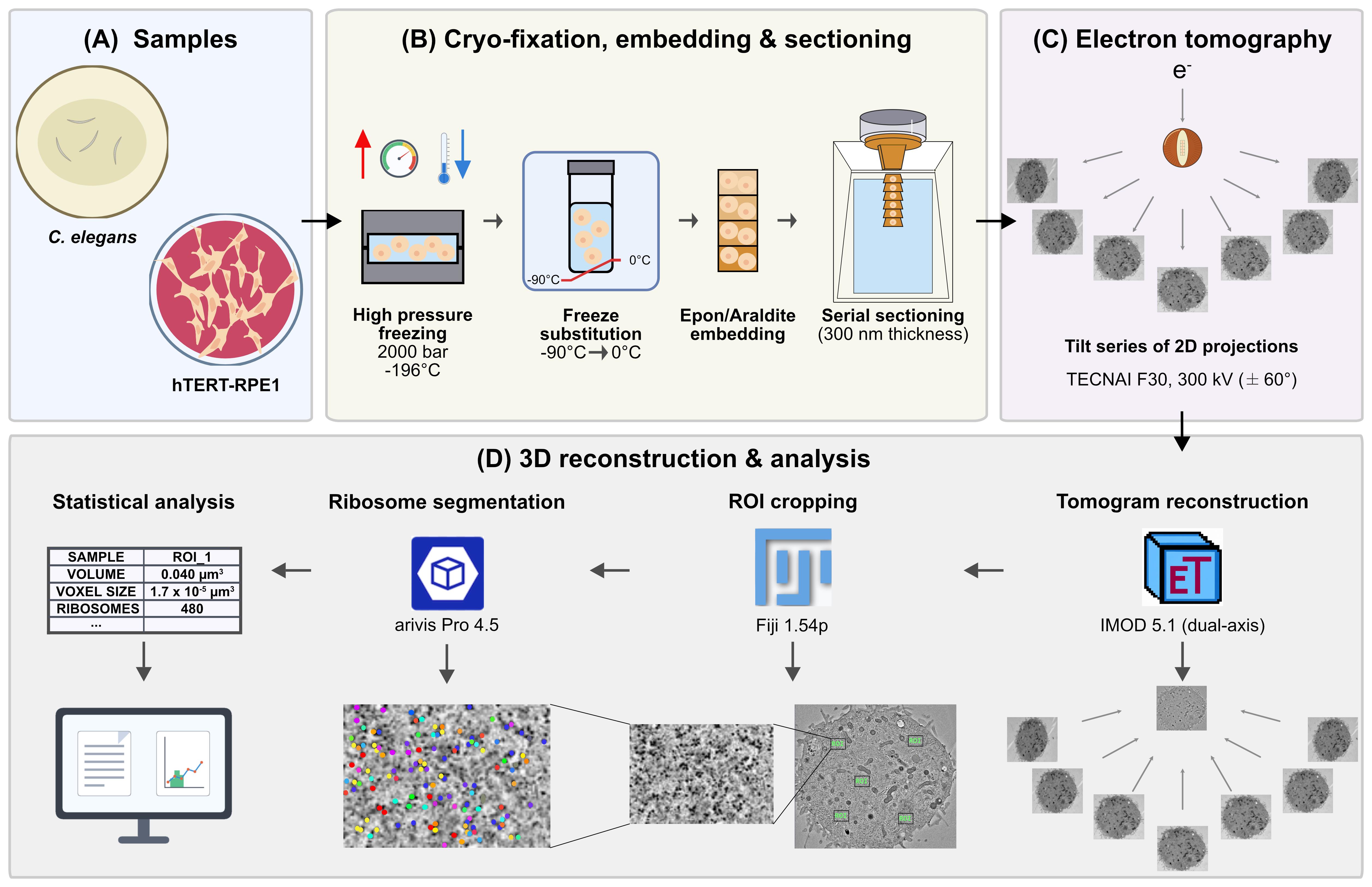
Graphical overview of the global workflow to count ribosomes in cellular sub-volumes. (A) Samples: hTERT-RPE-1 cells and Caenorhabditis elegans. (B) Cryo-fixation, embedding, and sectioning: high-pressure freezing (HPF, approximately 2,000 bar, -196 °C), freeze-substitution (FS, -90 to 0 °C), Epon/Araldite embedding, and serial sectioning (300 nm). (C) Electron tomography: dual-axis tilt-series of 2D projections on a TECNAI F30 at 300 kV (±60°). (D) 3D reconstruction and analysis: tomogram reconstruction in IMOD 5.1 (dual-axis), ROI cropping in Fiji 1.54p, ribosome segmentation in arivis Pro 4.5, and statistical analysis relating voxel size, ROI volume, and ribosome number.
Background
Ribosome abundance profoundly influences growth, development, and proteome output, yet robust in situ quantification across single cells and tissues remains challenging. Traditional biochemical rRNA measurements such as capillary electrophoresis, ribosomal protein quantification, and bulk estimates provide population-level readouts but suffer from extraction losses, protocol-dependent bias, and poor spatial resolution in heterogeneous tissues [1]. Although cryo-electron tomography (cryo-ET) has been used to segment ribosomes in focused ion beam (FIB)-milled lamellae of vitrified cells [2–6], it requires expensive equipment and expert knowledge and is limited to a relatively small field of view. Additionally, cryo-ET entails complications, such as ice contamination, low signal-to-noise ratios, and low throughput. To address these limitations, we developed an electron tomography-based pipeline to count ribosomes directly within preserved cellular volumes [1]. The present protocol focuses on the computational workflow for segmenting ribosomes in resin-embedded samples. The underlying sample preparation uses high-pressure freezing (HPF) and freeze-substitution, building on our established procedures for C. elegans [7] and adherent mammalian cells [8], and the specific implementation for ribosome quantification is documented in the primary study [1]. This workflow makes robust ribosome quantification accessible to a much broader audience without requiring specialized cryo-EM equipment. A limitation of this approach is that heavy-metal staining labels nucleic acids and proteins nonspecifically, so assembled ribosomes cannot be distinguished from similarly sized globular densities on the basis of contrast alone. False positives (e.g., unassembled subunits, proteasomes, major vault proteins, glycogen granules) and false negatives (ribosomes lost in regions of poor contrast) are therefore expected. We mitigate this in three ways: by bracketing the result across several voxel-count thresholds rather than reporting a single value (section D9), by validating against an independent biochemical measurement of rRNA by capillary electrophoresis, and by confirming that a genetic perturbation of ribosome biogenesis, rpoa-1(RNAi), shifts the density in the expected direction.
Materials and reagents
To provide a standalone, end-to-end workflow, all biological materials, reagents, laboratory supplies, and recipes required for the sample preparation steps (section A) and the computational segmentation are listed below. For extended background, rationale, and troubleshooting on the cryo-preparation itself, see Fabig et al. (2019) [7], Section 3.2, for C. elegans, and Kiewisz et al. (2023) for mammalian cells [8].
Biological materials
1. hTERT-RPE-1 cells, human retinal pigment epithelial cells (ATCC, catalog number: CRL-4000) [1]
2. Caenorhabditis elegans, wild type (N2, Bristol) (Caenorhabditis Genetics Center, CGC) [1,7]
3. Escherichia coli OP50 (Caenorhabditis Genetics Center, CGC) [1,7]
4. Escherichia coli HT115(DE3) (Caenorhabditis Genetics Center, CGC) [1]
5. pL4440 RNAi vector (Addgene, plasmid number: 1654). The rpoa-1 construct targets RPOA-1, the largest subunit of C. elegans RNA polymerase I in order to inhibit ribosome biogenesis. It was generated by cloning nucleotides 4073–5115 of transcript Y48E1A.1a.1 into pL4440. Forward primer: 5′-TGCACTTGTTCGTCGATCCA-3′; reverse primer: 5′-GAGAAGACGGTCCTGCAACA-3′ [1]
Reagents
1. Acetone (CH3COCH3), glass-distilled, EM grade (EMS, Electron Microscopy Sciences, catalog number: 10015)
2. Araldite 502, Embed 812, Embedding kit with DMP (Science Services, catalog number: E13940-DMP)
3. BSA (albumin fraction V) (Carl Roth, catalog number: 8076.2)
4. Chloroform (CHCl3) (EMS, catalog number: 12550)
5. Colloidal gold solution, diameter 20 nm (BBI Solutions, catalog number: EM.GC20/4)
6. DAPI (Sigma-Aldrich, catalog number: D9542)
7. Disodium hydrogen phosphate (Na2HPO4) (Carl Roth, catalog number: P030.2)
8. DMEM, high glucose, GlutaMAX Supplement (Thermo Fisher Scientific, catalog number: 10566016)
9. Fetal bovine serum (FBS), heat-inactivated, origin: USA (Thermo Fisher Scientific, catalog number: 10082147)
10. Formvar (Science Services, catalog number: E15800)
11. 1-Hexadecene (Merck, catalog number: 8.22064.0500)
12. Isopropyl-β-D-thiogalactopyranoside (IPTG) (Sigma-Aldrich, catalog number: I1284)
13. Lead citrate (C12H10O14Pb3) (Science Services, catalog number: E17810)
14. Magnesium sulphate heptahydrate (MgSO4·7 H2O) (Carl Roth, catalog number: P027.1)
15. MemBrite Fix 543/560 Cell Surface Staining kit (Biotium, catalog number: 30094-T)
16. Methanol (CH3OH) (VWR, catalog number: 20834.291)
17. Osmium tetroxide (OsO4) (Science Services, catalog number: E19100)
18. Penicillin-streptomycin-glutamine (100×) (Thermo Fisher Scientific, catalog number: 10378016)
19. Poly-L-lysine (0.1% w/v in H2O) solution (Sigma-Aldrich, catalog number: P8920-100ML)
20. Polyvinylpyrrolidone (PVP), Avg. Mol. Wt. 10,000 (Sigma-Aldrich, catalog number: P2307-100G)
21. Potassium dihydrogen phosphate (KH2PO4) (Carl Roth, catalog number: 3904.1)
22. Sodium chloride (NaCl) (Merck, catalog number: 106404)
23. Trypsin-ethylenediaminetetraacetic acid (EDTA) (0.25%) (Thermo Fisher Scientific, catalog number: 25200056)
24. Uranyl acetate [UO2(CH3COO2)] 98%, ACS reagent (Polysciences, catalog number: 21447-25)
Caution: Osmium tetroxide, uranyl acetate, lead citrate, chloroform, and methanol are toxic and/or volatile. Uranyl acetate is additionally weakly radioactive. Handle all of these in a fume hood with appropriate personal protective equipment and dispose of waste according to institutional regulations.
Solutions
1. Automatic freeze-substitution (AFS) cocktail (see Recipes)
2. DMEM-WT (see Recipes)
3. DMEM-HPF cryoprotectant solution (see Recipes)
4. Epon/Araldite resin (see Recipes)
5. Formvar solution (see Recipes)
6. Lead citrate post-staining solution (see Recipes)
7. M9 buffer (see Recipes)
8. Uranyl acetate post-staining solution (see Recipes)
9. Worm cryoprotectant solution (see Recipes)
Note: The essential recipes for these solutions, post-stains, and embedding resin are provided in the Recipes section below to allow for a standalone workflow. For comprehensive background, rationale, and extensive troubleshooting on these specific sample preparation steps, please refer to Fabig et al. (2019) [7] and Kiewisz et al. (2023) [8].
Recipes
1. AFS cocktail
| Reagent | Final concentration | Quantity or volume |
|---|---|---|
| Osmium tetroxide | 1.0% (w/v) | 0.50 g |
| Uranyl acetate | 0.1% (w/v) | 0.05 g |
| Acetone | n/a | to 50 mL |
| Total | n/a | 50 mL |
Note: Aliquot 1 mL each in 2 mL cryotubes, freeze them immediately in liquid nitrogen, and store them in liquid nitrogen until further use.
2. DMEM-WT (standard medium for mammalian cell culture)
| Reagent | Final concentration | Quantity or volume |
|---|---|---|
| FBS | 10% (v/v of DMEM) | 50 mL |
| Penicillin-streptomycin-glutamine | 1% (v/v of DMEM) | 5 mL |
| DMEM | n/a | 500 mL |
| Total | n/a | 555 mL |
3. DMEM-HPF cryoprotectant solution
| Reagent | Final concentration | Quantity or volume |
|---|---|---|
| BSA | 10% (w/v) | 1 g |
| DMEM-WT | n/a | to 10 mL |
| Total | n/a | 10 mL |
4. Epon/Araldite resin
| Reagent | Final concentration | Quantity or volume |
|---|---|---|
| Embed 812 | n/a | 31.02 g |
| Araldite 502 | n/a | 22.20 g |
| DDSA (dodecenyl succinic anhydride, supplied with the kit) | n/a | 61.00 g |
| DMP-30 (2,4,6-tris(dimethylaminomethyl)phenol, supplied with the kit) | n/a | 2.67 g |
| Total | n/a | 116.89 g |
Mix all reagents in a single-use plastic beaker with a magnetic stirrer overnight. The next day, fill up 10 mL syringes with mixed resin, close them with paraffin, and store them at -20 °C until further use.
Note: All four components are supplied in the Araldite 502/Embed 812 Embedding kit with DMP.
5. Formvar solution
| Reagent | Final concentration | Quantity or volume |
|---|---|---|
| Formvar powder | 1% (w/v) | 1 g |
| Chloroform | n/a | 100 mL |
| Total | n/a | 100 mL |
Note: To coat grids, dip a clean glass slide into the Formvar solution, air-dry, and float the resulting film onto the surface of a clean water bath. Place slot grids onto the floating film, collect film with a glass slide, and dry before use.
6. Lead citrate post-staining solution
| Reagent | Final concentration | Quantity or volume |
|---|---|---|
| Lead citrate | 0.4% (w/v) | 0.2 g |
| diH2O | n/a | 50 mL |
| Total | n/a | 50 mL |
7. M9 buffer
| Reagent | Final concentration | Quantity or volume |
|---|---|---|
| KH2PO4 | 22.0 mM | 3 g |
| Na2HPO4 | 42.3 mM | 6 g |
| NaCl | 85.6 mM | 5 g |
| MgSO4·7 H2O | 1.0 mM | 0.25 g |
| diH2O | n/a | to 1,000 mL |
| Total | n/a | 1,000 mL |
8. Uranyl acetate post-staining solution
| Reagent | Final concentration | Quantity or volume |
|---|---|---|
| Uranyl acetate | 2% (w/v) | 0.2 g |
| Methanol | 70% (v/v) | 7 mL |
| diH2O | n/a | to 10 mL |
| Total | n/a | 10 mL |
9. Worm cryoprotectant solution
| Reagent | Final concentration | Quantity or volume |
|---|---|---|
| PVP | 10% (w/v) | 1 g |
| M9 buffer | n/a | 10 mL |
| Total | n/a | 10 mL |
Laboratory supplies
1. Sapphire discs for high-pressure freezing (diameter 3 mm, thickness 0.16 mm) (Wohlwend GmbH, catalog number: Article 500)
2. Aluminum specimen carriers for high-pressure freezing (diameter 3 mm, cavity 40/600 μm, thickness 0.84 mm) (Wohlwend GmbH, catalog number: Article 737)
3. Type-A aluminum specimen carriers for high-pressure freezing (diameter 3 mm, cavity 100/200 μm, thickness 0.50 mm) (Wohlwend GmbH, catalog number: Article 241)
4. Type-B aluminum specimen covers (flat at one side) for high-pressure freezing (diameter 3 mm, cavity 300 μm, thickness 0.50 mm) (Wohlwend GmbH, catalog number: Article 242)
5. Nematode growth medium (NGM) agar plates (prepared in-house according to [9])
6. Gilder single oval 2 mm slot copper TEM support grids (Electron Microscopy Sciences, catalog number: G2010-Cu)
7. Grid storage box, 100-capacity (Electron Microscopy Sciences, catalog number: 71155)
8. Cell culture flask, 250 mL, 75 cm2 (T75), polystyrene, sterile, with red filter screw cap (Greiner Bio-One, catalog number: 658175)
9. Cryotubes, 2 mL (Greiner Bio-One, catalog number: 126261)
10. Disposable syringes, 10 mL (B. Braun, catalog number: 4617100V-02)
11. Parafilm M (Pechiney, catalog number: HS234526A)
12. Filter paper (Sigma-Aldrich, catalog number: WHA1540090)
13. Syringe filters, 0.2 μm (Sarstedt AG, catalog number: 83.1826.001)
Equipment
1. High-pressure freezer (Wohlwend, model: HPF Compact 03) [1,8]
2. Automatic freeze-substitution system (Leica Microsystems, model: EM AFS2) [1,7,8]
3. Ultramicrotome (Leica Microsystems, model: EM UC6) [1,8]
4. Transmission electron microscope for tomography (Thermo Fisher Scientific, model: TECNAI F30, 300 kV) [1,7,8]
5. Transmission electron microscope for screening (Thermo Fisher Scientific, model: Morgagni, 80 kV) [1]
6. sCMOS camera (Gatan, model: OneView, 4k × 4k) [1,7,8]
7. CCD camera (EMSIS, model: Veleta, 2k × 2k) [1]
8. Dual-axis specimen holder (Fischione Instruments, model: Type 2040) [1]
9. Confocal microscope (Leica Microsystems, model: TCS SP5) with a 40×/1.25 HCX PL APO lambda blue oil objective [1]
10. Bioanalyzer (Agilent, model: 2100) with RNA 6000 Nano Kit (Agilent) [1]
11. Centrifuge (5702 R) (Eppendorf, catalog number: 5703000010)
12. Incubator cell culture (TECO 20) (Selutec, catalog number: 600.005)
Software and datasets
1. arivis Pro [10] (segmentation), 4.5, 2024, commercial, paid (license required), https://www.zeiss.com/microscopy/de/produkte/software/arivis-pro.html
2. IMOD [11, 12] (reconstruction, mrc2tif), 5.1, 2024, GPL, free, https://bio3d.colorado.edu/imod/download.html
3. SerialEM [13, 14] (acquisition), 3.x, 2020–2024, free for academic use, https://bio3d.colorado.edu/SerialEM/download.html
4. Fiji [15] (ROI cropping), 1.54p, 2025, GPL, free, https://imagej.net/software/fiji/downloads
5. RStudio (statistics), R 4.4.1; RStudio 2024.12.0, 2024, open source, free, https://posit.co/products/open-source/rstudio
6. Tomogram and segmentation datasets, n/a, 2024–2025, open access, free (OMERO; accession IDs in Supplementary) [1], https://omero.med.tu-dresden.de/webclient/?show=project-1303
Note: The primary study used arivis Vision4D 3.4 and 3.5 [1]. This protocol is written for the current arivis Pro 4.5, with menu terminology updated accordingly, while parameter values remain unchanged. Free alternatives such as Fiji with TrackMate or the 3D ImageJ Suite, or ilastik, can be adapted but require independent re-validation.
Procedure
Notes:
1. Condensed but executable procedures are given for the experimental steps in section A, with the primary publications retained as pointers for extended background, rationale, and troubleshooting.
2. Recommended parameter values are compiled in Table 1 and reiterated at the corresponding protocol steps.
3. Software menu, box, and button names are formatted in italics; operation step titles are in bold italics.
Table 1. Recommended parameters, as used in the validation study [1]
| Parameter | Value |
|---|---|
| Section thickness | 300 nm |
| TEM voltage | 80 kV (screening); 300 kV (tomography) |
| Tilt range and increment | -60° to 60° (dual-axis), 1° |
| Magnification and pixel size | 4,700×, 2.572 nm |
| Target defocus | -4 μm |
| Target mean counts | 45,000 (taper to 40,000 above ±50°) |
| Drift settling (for record) | 1.0 s |
| Fiducials | 20 nm colloidal gold on both sides |
| Shrinkage factor (laboratory) | 1.575, from 77 stitched datasets, applied in Z |
| Denoising | Median filter, diameter 7.72 nm, rank 50% |
| Blob Finder | Diameter 30 nm, probability 30%, split sensitivity 70% (detects 1–30 nm) |
| Voxel thresholds (voxel-size dependent; recompute for other pixel sizes; see section D9) | Lower 25, 50, 100 (empirical; theoretical 150 excluded structures identifiable as ribosomes); exclude above 830 |
A. Sample preparation and tomography acquisition
1. hTERT-RPE-1 cell culture, mitotic shake-off, and HPF:
a. Grow cells in T75 flasks (37 °C, 5% CO2).
b. Harvest mitotic cells by performing a mitotic shake-off, collect the medium containing the detached cells, and centrifuge (at 300 rcf for 5 min) to pellet.
c. Resuspend the cell pellet in DMEM-WT and seed the cell suspension onto poly-L-lysine-coated sapphire discs.
d. Place the seeded discs in an incubator (37 °C, 5% CO2) for 15 min to allow the cells to settle and adhere.
e. Assemble the specimen carrier sandwich using the sapphire disc and a specimen carrier with a cavity depth of 40 µm.
f. Use DMEM-HPF solution as cryoprotectant, ensuring that it completely fills all spaces within the sandwich. Residual air pockets prevent proper heat transfer and cause ice-crystal damage during freezing.
g. Freeze at approximately 2,000 bar using a high-pressure freezer [1,8].
Critical: Harvest cells by mitotic shake-off, not by trypsin, because trypsin-EDTA induces ribosome clustering that biases quantification [16]. Trypsin (0.25%) is used only for the confocal cell-volume measurement (section E).
Notes:
1. While the essential, actionable steps are provided above, readers should refer to Kiewisz et al. (2023) [8] for comprehensive background (Procedure sections A and B), rationale, and visual troubleshooting (see Graphical overview and Figures 1–2) for cell culture, coating, shake-off, and sandwich assembly.
2. To coat sapphire discs, incubate them in 0.1% (w/v) poly-L-lysine solution for 5 min at room temperature, remove the excess solution with filter paper, and dry the discs for 2 h at 60 °C [8].
2. C. elegans culture and HPF:
a. Maintain N2 worms on OP50-seeded NGM agar plates at 20 °C.
b. Induce dsRNA expression with 1 mM IPTG and feed approximately 40 L4 animals with E. coli pL4440 vector (empty for control or rpoa-1 inserted for knockdown) for 24 h at 25 °C [17,18].
c. Precoat type-A specimen carriers with 1-hexadecene and fill the 100 µm cavity with worm cryoprotectant solution.
d. Transfer approximately five gravid adult hermaphrodites (24 h post-L4) per type-A carrier, close with the flat side of a type-B specimen cover.
e. Freeze at approximately 2,000 bar as in step A1 [1,7].
Note: Please refer to Fabig et al. (2019) [7] for additional methodological context (section 2.2) and visual guides (see Graphical overview) on worm handling and loading. As established in that study, utilizing PVP at 10% (w/v) yields excellent freezing and enables the recovery of structurally intact worms after freeze-substitution.
3. Freeze-substitution (FS), embedding, sectioning, and post-staining:
a. Perform FS in AFS cocktail using an AFS system: hold at -90 °C for 1 h, warm to -30 °C at 5 °C/h, hold at -30 °C for 5 h, then warm to 0 °C at 5 °C/h.
b. Infiltrate and embed samples in Epon/Araldite resin, polymerize at 60 °C for 48 h, cut 300 nm serial sections and collect them onto Formvar-coated copper slot grids (2 mm single oval slot; coated in-house with Formvar; see Laboratory supplies and Reagents).
c. For post-staining, pre-wash grids in 70% methanol for 2 min, then incubate in freshly prepared, 0.2 µm-filtered uranyl acetate post-staining solution for 10 min.
d. Wash the grids sequentially (3 × 1 min per step) in 70%, 50%, and 30% methanol, followed by 3 × 1 min washes in deionized water (diH2O).
e. Next, stain with 0.2 µm-filtered lead citrate post-staining solution for 5 min, wash 3 × 1 min in diH2O, and air-dry.
f. To apply fiducial markers, immerse the grid into a droplet of 20 nm colloidal gold solution for 1 min.
g. Blot excessive fluid with filter paper and air-dry the grid for 1 min.
h. Submerge the grid for 1 min in a droplet of deionized water and let it air-dry before storing it in a grid box [1].
Notes:
1. The actual section thickness might differ from the thickness set on the ultramicrotome (e.g., due to ambient thermal fluctuations or vibrations). To estimate the section thickness during ultramicrotomy, the interference color chart from RMC Boeckeler (Figure 1) serves as a reliable reference. This allows for the rapid screening and exclusion of excessively thin or thick sections prior to electron microscopy.
2. For extensive background, rationale, and detailed troubleshooting regarding these freeze-substitution, embedding, and sectioning parameters, see Müller-Reichert et al. (2003) [19] and Fabig et al. (2019) [7] for worms, and Kiewisz et al. (2023) [8] for cells.
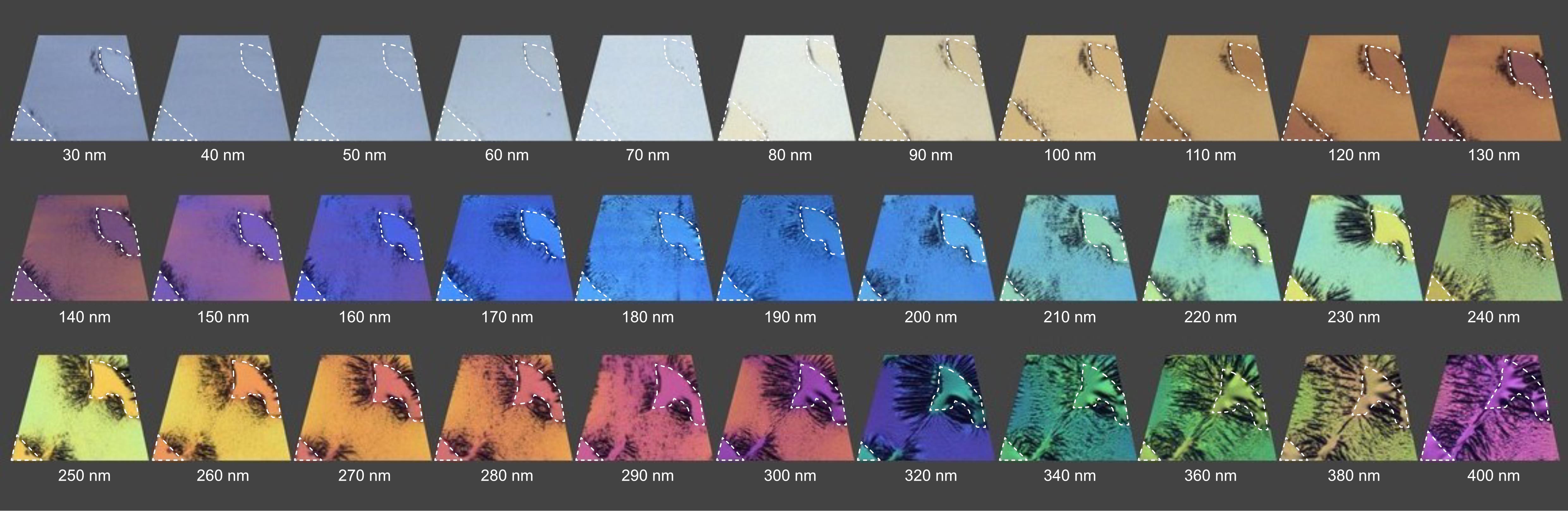
Figure 1. Relationship between section thickness and the interference color of Epon sections. The provided example shows a mouse spleen embedded in Embed 812 epoxy resin, where the area within the dashed lines represents empty resin. Thicknesses from 30 to 400 nm are shown. Image modified from https://boeckeler.com/wp-content/uploads/2022/05/AN_Powertome_Ultrathin-Section-Thickness-and-Interference-Color-and-Chart.pdf, reproduced with kind permission from RMC Boeckeler.
4. Dual-axis electron tomography:
a. Prescreen sections on a Morgagni TEM operated at 80 kV to locate interphase hTERT-RPE-1 cells and C. elegans distal-gonad, pachytene, and vulva cells.
b. Acquire dual-axis tilt series with camera parameters as indicated in Figure 2A on a TECNAI F30 at 300 kV over -60° to 60° in 1° increments at 4,700× and a pixel size of 2.572 nm using SerialEM. Use the settings for the tilt series acquisition as shown in Figure 2B.
c. For the second axis, rotate the grid by 90° within the holder cartridge by turning the knob outside of the Fischione 2040 holder. The holder has a built-in detent that the user feels when approaching 90° and then snaps into position at exactly 90°.
d. Relocate the region of interest recorded in the first-axis tilt series, then re-establish eucentric height and re-run the tilt series with identical settings [1,13,14].
Note: Before acquiring a tilt series for each position for the first time, pre-irradiate the area for 5 min at -60° tilt and at 2,700× magnification to stabilize the section against beam-induced collapse. For extended background on pre-irradiation, see Kiewisz et al. (2023), Procedure step D19 [8].
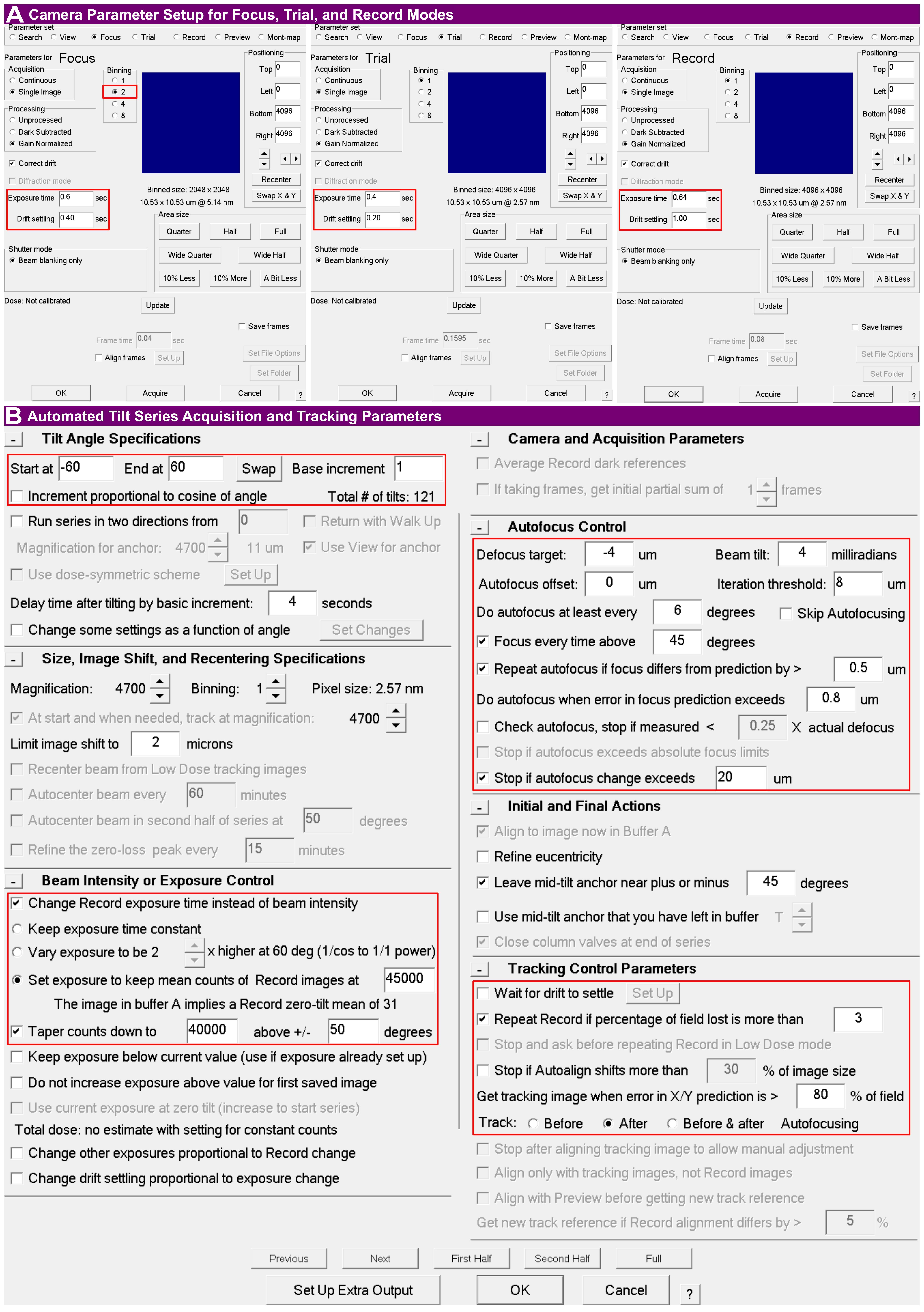
Figure 2. SerialEM tilt series acquisition parameters. (A) Camera setup configurations for focus, trial, and record modes. Key parameters such as binning, exposure time, and drift settling (e.g., 1.00 s for record) are highlighted. (B) Main tilt series setup dialog configuring the automated acquisition scheme. Highlighted regions denote the unidirectional tilt scheme (-60° to 60° with 1° increments), dynamic exposure control to maintain mean image counts, autofocus control (target defocus of -4 µm, autofocus at least every 6°, and Focus every time above 45 degrees enabled), and tracking control (Track: After Autofocusing, a new tracking image acquired when the X/Y prediction error exceeds 80% of the field, and record repeated if more than 3% of the field is lost).
B. Tomogram reconstruction and combination (IMOD 5.1, dual-axis)
Note: Reconstruction, combination, flattening, and trimming are performed using IMOD [11,12]. The workflow is summarized in Figures 3 and 4. After recording a tilt series, the images are stored in the MRC file format, which Etomo requires as input.
1. Configure Etomo settings: When starting Etomo for the first time, go to Options > Settings to enable GPU processing and/or set the number of parallel CPU cores that should be used (Figure 3A).
2. Project setup: Open Etomo. On the Front Page (active state), click Build Tomogram. In the Setup Tomogram window, load the raw image stack for Axis A and enter the fiducial diameter for the 20 nm colloidal gold. Click Scan Header to populate the pixel size and image rotation from the stack header. Confirm that the axis and frame settings match your data acquisition parameters; for the standard workflow and example dataset presented here, select Dual axis and Single frame. Leave Series was bidirectional unchecked for a unidirectional tilt series. Ensure Parallel Processing and Graphics card processing are enabled, and then click Create Com Scripts (Figure 3B–C).
3. Open the process manager: Open the Main Process Manager (dual-axis) and click Both under Axis A to display the process managers for both axes (Figure 3D).
4. Pre-processing: Under the CCD Eraser tab, click Find X-rays (Trial Mode), followed by Create Fixed Stack, and finally click Done to remove X-ray and hot pixels (Figure 3E).
5. Coarse alignment: Run Calculate Cross-Correlation, click Generate Coarse Aligned Stack, and then click Done (Figure 3F).
6. Fiducial model generation and fine alignment: Generate the Seed Model automatically by entering a Total number of fiducial seed points. Activate Refine center with Sobel filter and (if applicable) select Select beads on two surfaces (Figure 3G). Click Generate Seed Model to find beads, and then click Done.
Note: We recommend a target count of 60 seed points, which is optimized for a standard area of approximately 100 μm2 (adjust proportionately for different field-of-view areas). Note that entering this target count assumes that a sufficient number of fiducials is physically present and visible in the field of view; the algorithm will attempt to find this quantity.
7. Fiducial tracking: Under the Track Beads tab, click the A button to display advanced options (Figure 3H). Increase the Rounds of tracking to ≥10. Click Track Seed Model, and then repeatedly click Track with Fiducial Model as Seed (≥10 times) until the reported number of untracked beads stabilizes. To monitor this number, check the Etomo process log window (accessed and displayed by pressing Ctrl + L) after each run.
Note: If automatic fiducial tracking fails or a high number of untracked beads remains in the log window, use the Fix Fiducial Model function to open the model in 3dmod. Manually patch gaps or delete aberrant points, save the model, and re-run the tracking.
8. Run Fine Alignment (Tiltalign). Under the Global Variables tab, enable Distortion > Full solution. Then, navigate to the Projection Stretch section of the same tab, click the A button to display advanced options, and enable Solve for single stretch during projection. Return to the General tab (Figure 3I), select Assume fiducials on 2 surfaces for analysis, enable Do robust fitting with tuning factor (1.0), and select Enable local alignments (target patch size 700 × 700 px; minimum 10 fiducials total, 4 per surface). Click Compute Alignment, then click Done. Optionally inspect the result with View Residual Vectors or View 3D Model before proceeding.
Note: These specific global variables are critical for resin-embedded sections. Full solution corrects for non-isotropic magnification and electromagnetic lens distortions across the tilt series, while Solve for single stretch mathematically compensates for the physical thinning and shrinkage of the resin section as it is exposed to the electron beam.
9. Axis B setup and fiducial transfer: For Axis B, follow the steps similarly to Figure 3E–F. To perform fiducial transfer from Axis A, navigate to the Seed Model tab, select Make seed and track, select Transfer seed model from the other axis, click Transfer Fiducials From Other Axis, and click Done (Figure 3J). Then, repeat steps B7 (Figure 3H) and B8 (Figure 3I). All following steps are similar for both axes.
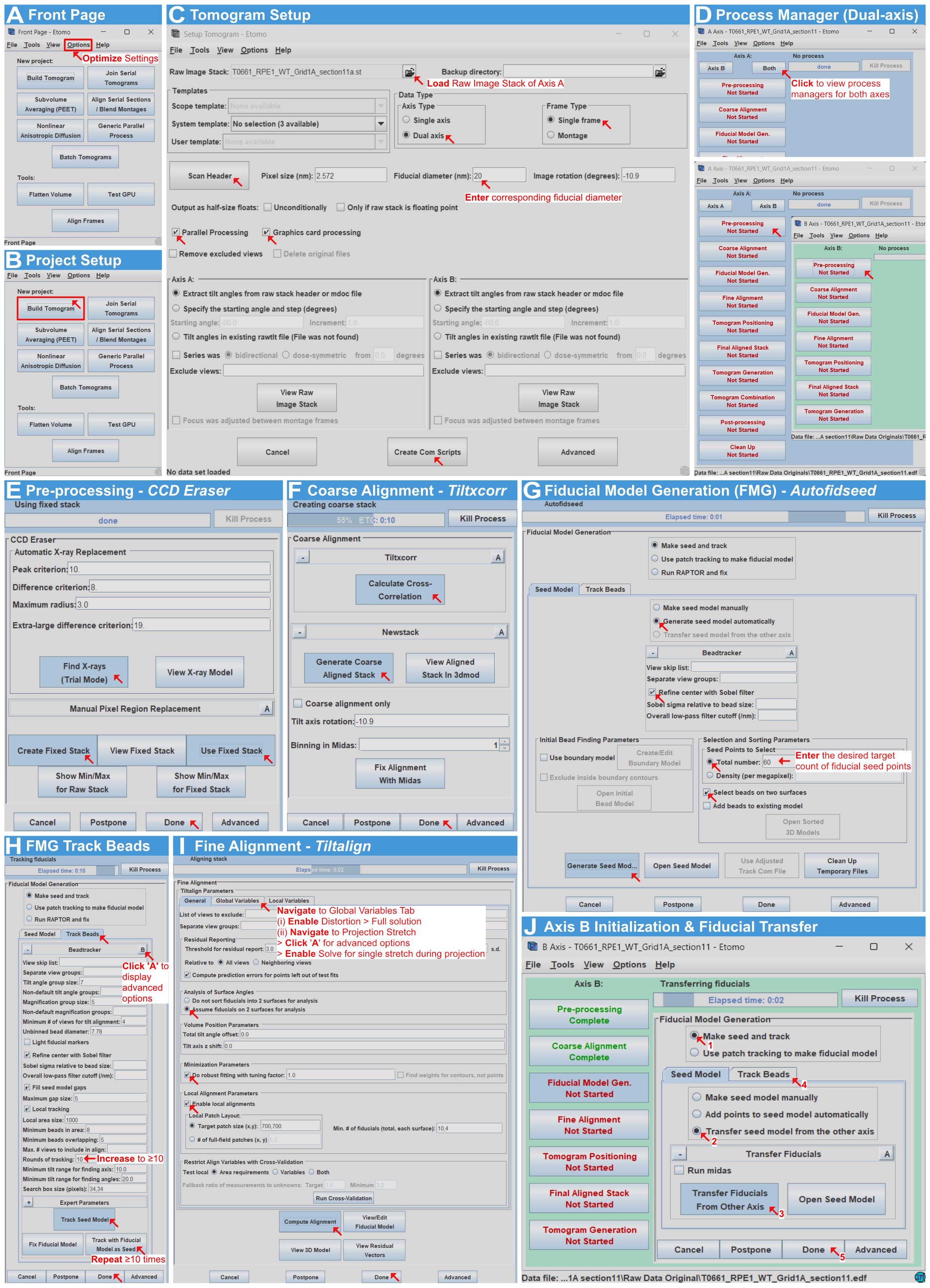
Figure 3. Fiducial-based alignment of dual-axis electron tomograms in IMOD. (A) Front Page (initial state): Optimize settings via Options. Enabling GPU or multi-core CPU processing reduces processing time. (B) Setup tomogram window with optimized settings applied. (C) Setup tomogram configuration based on image acquisition parameters (e.g., dual-axis, single frame, and the specific diameter of gold fiducials). Parallel processing options are enabled. (D) Main Process Manager displaying the setup for both dual-tilt axes. The following steps must be performed for both axes but are illustrated here for Axis A only. (E) Preprocessing with CCD Eraser to remove X-ray and hot pixels. (F) Coarse alignment using Tiltxcorr and Newstack. (G) Fiducial model generation (Seed Model), indicating where to enter the recommended target count (e.g., 60) of fiducial seed points. (H) Fiducial tracking. Advanced options are displayed to increase the rounds of tracking (e.g., ≥10 times), and tracking is repeated until the number of untracked beads stabilizes. (I) Fine alignment (Tiltalign). Critical parameters are enabled under the Global Variables and Projection Stretch (advanced options) tabs, alongside robust fitting and local alignments. (J) Axis B fiducial transfer. This is the only difference between the reconstruction workflows of the two axes; the second axis utilizes the fiducial model transferred from the first axis (rotated by ~90°).
10. Tomogram positioning and final alignment: Under the Tomogram Positioning tab, select Use the GPU and Find boundary model automatically. To prevent clipping of tilted sections, increase the Positioning tomogram thickness (e.g., to 1,000). Select Use whole tomogram with Binning set to 3, add extra padding by increasing the Added border thickness (unbinned) (e.g., to 50), and click Create Tomogram & Boundary Model (Figure 4A, steps 1–6). Click View Boundary Model to open the binned tomogram in 3dmod (Figure 4A, step 7). To flip the tomogram for the side-on view, click Edit > Image > Flip/Rotate. Position the contour points at the upper and lower specimen boundaries, and check/correct the contours of the boundary model (Figure 4B). Save and close the model. Return to Etomo and click Compute Z Shift & Pitch Angles. Explicitly increase the Final Tomogram Thickness (consider doubling the suggested value displayed) to ensure the full volume is captured, and click Create Final Alignment (Figure 4A, steps 8–10).
Note: These values are appropriate for 300 nm sections at a pixel size of 2.572 nm. Scale the positioning thickness and final tomogram thickness to your own section thickness and pixel size; the goal is simply to leave sufficient Z-range that no specimen data is clipped during positioning or reconstruction.
11. Final aligned stack generation: Under the Create tab, enable Use linear interpolation to reduce noise, and ensure Aligned image stack binning is set to 1. Finally, click Create Full Aligned Stack (Figure 4C).
12. Tomogram generation. Select Back Projection and ensure Standard ramp function and Standard Gaussian (cutoff 0.35, falloff 0.035) are selected. Ensure the following checkboxes are selected: Use the GPU, Take logarithm of densities (with offset 0.0), Use local alignments, and Use Z factors. Finally, click Generate Tomogram (Figure 4D).
13. Tomogram combination: On the Setup tab, set Used # Cores to the maximum number of cores and Nice to 0 (default 15) for maximum priority. Select Match the B tomogram to A and Fiducials on both sides. Set Patch Size to Small patches and Max Patch Size to Extra large patches. Click 3dmod Volume A to inspect the volume, then enter the in-focus Z-axis min and Z-axis max values (e.g., 110 and 190); the X and Y limits are populated automatically. Then, click Create Combine Scripts followed by Start Combine (Figure 4E). The Initial Match and Final Match tabs proceed automatically unless an error occurs (Figure 4F–G). If Combine or Matchorwarp fails, right-click the interface and select Show Log. Scroll to the bottom of the log to locate the software’s directly suggested value. Enter this recommended value in the corresponding field: Limit on maximum residual on the Initial Match tab, or Warping residual limits on the Final Match tab, and click Restart Combine or Restart at Matchorwarp, respectively.
14. Preview the combined volume: Once combination is complete, click Open Combined Volume to preview the reconstructed tomogram combination (Figure 4H).
15. Post-processing and volume trimming: Ensure that the Subarea and Float options are selected in the 3dmod window (Figure 4I). Use the Rubberband tool to outline the cell in the preview window (which automatically populates the Subarea coordinates) and use the Z slider to identify the top and bottom limits before the tomogram becomes blurry near the section edges. To accommodate the algorithmic flattening process without clipping specimen data, first expand the in-focus Z-range by approximately 50 Z-slices on the top and bottom of the tomogram. Also, note the minimum (black) and maximum (white) values within those bounds and enter these under Volume Range and Scaling together with Convert to bytes (e.g., black 201, white 234; Figure 4I). Do not change the pre-set Reorientation method, which is Rotate around X axis; as the interface warns, the same reorientation method must be used for every section in a serial join. Then, click Trim Volume (Figure 4I). Perform optional flattening if the physical section appears warped or bent along the Z-axis.
Notes:
1. Detailed step-by-step procedures for executing the flattening process (e.g., generating surface contours and utilizing the Flatten tab in Etomo) are beyond the scope of this protocol. Users requiring this step should refer to the official IMOD Tomography Guide (https://bio3d.colorado.edu/imod/doc/tomoguide.html#Flattening).
2. It is not strictly necessary to trim the tomogram boundaries specifically to remove surface fiducial markers; any remaining gold beads will not interfere with the downstream ribosome particle picking.
16. Export: The combined and trimmed tomographic volume is saved as an 8-bit MRC stack. Convert MRC to TIFF for downstream processing. To avoid file conversion conflicts in the next steps, we recommend using the IMOD function mrc2tif for the conversion using default settings via the command line.
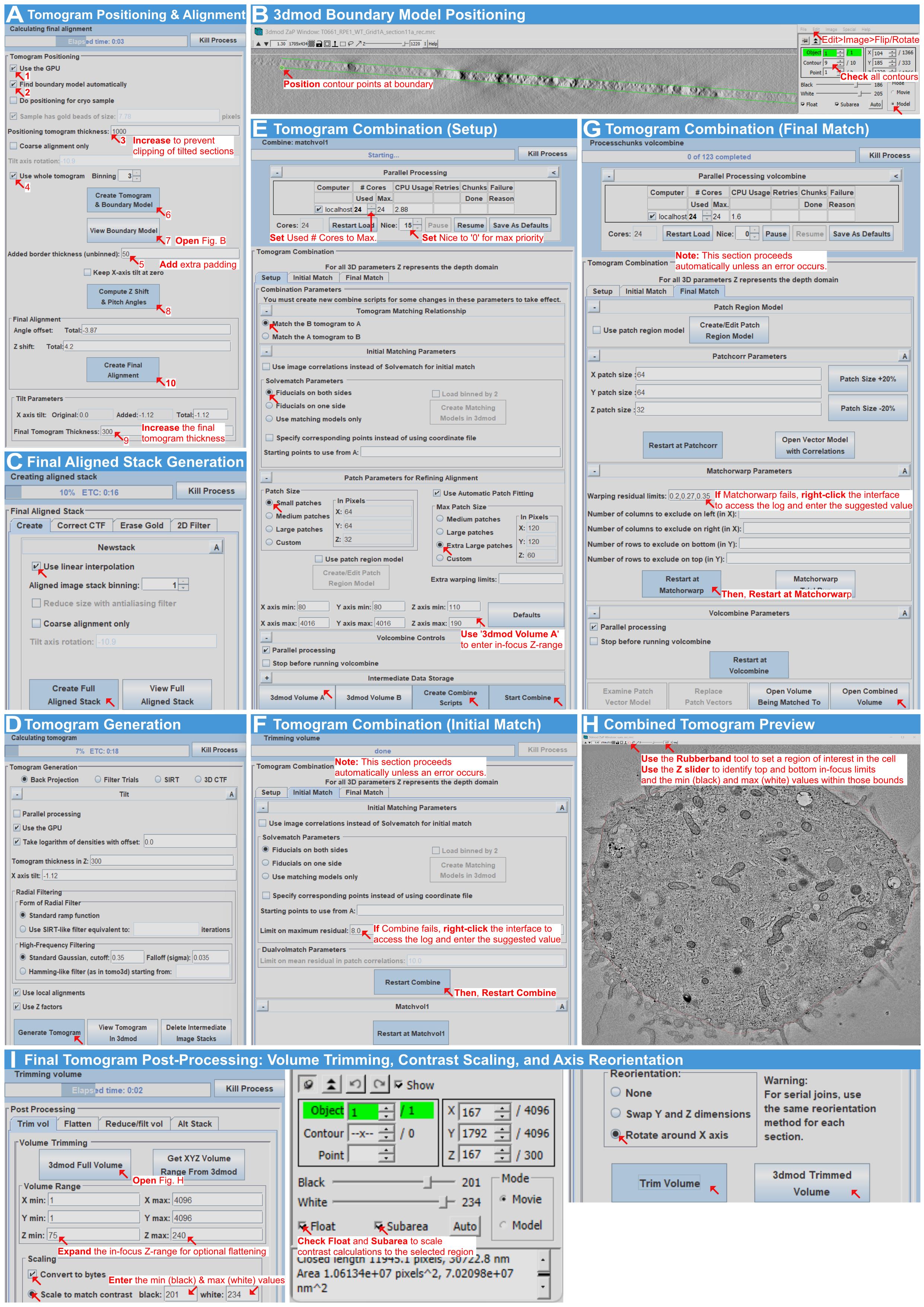
Figure 4. Tomogram positioning, dual-axis combination, and trimming in IMOD. (A) Tomogram positioning and final alignment. The Positioning tomogram thickness and Added border thickness are increased to prevent clipping and add padding, respectively, before generating the final alignment with an increased Final Tomogram Thickness. (B) 3dmod boundary model selection: flipping to the side-on view, positioning contour points at the specimen boundaries, and checking contours. (C) Generation of final aligned image stack, utilizing linear interpolation to reduce noise. (D) Tomogram generation using weighted back-projection. GPU processing and local alignments are enabled. (E) Tomogram combination (Setup tab). Processing priority is maximized (Used # Cores to Max # Cores, Nice to 0), and the in-focus Z-range is determined using 3dmod Volume A before creating combine scripts. (F) Tomogram combination (Initial Match tab). This proceeds automatically; if the combination fails, the error log is accessed (via right-click) to find a suggested value, which is entered before clicking Restart Combine. (G) Tomogram combination (Final Match tab). Similarly, if Matchorwarp fails, the log is used to find a recommended value before clicking Restart at Matchorwarp. (H) Preview of the reconstructed combined tomogram. (I) Post-processing and volume trimming. The Subarea and Float options are selected. The Rubberband tool defines the region of interest, and the Z slider identifies the top and bottom in-focus limits alongside min (black) and max (white) values. The in-focus Z-range is expanded for optional flattening before generating the final 8-bit trimmed tomogram.
C. ROI selection and cropping (Fiji)
Note: ROI selection and cropping are carried out in Fiji [15] and summarized in Figure 5.
1. Open the tomogram: Open the reconstructed tomographic TIFF stack in Fiji.
2. Select the ROI tool: Select the Rectangle selection tool (Figure 5, step 1) and zoom to 150% for precise ROI adjustment (Figure 5, step 2).
3. Choose the cytoplasmic region: Select an ideal cytoplasmic region containing predominantly ribosomes. To define the ROI, draw a square in 2D at the mid-plane of the tomogram, then scroll through the full Z-range to check for interfering structures (such as mitochondria, large vesicles, or other organelles) within the selected area. Because the cytoplasm is densely packed, minor intrusions are sometimes unavoidable. For example, the edge of a vesicle may slightly protrude into the ROI in part of the Z-stack, or a microtubule may cross the region. These do not need to be avoided entirely: subsequent filtering steps in the pipeline will remove most of these structures, and any remaining features (e.g., microtubules) can be manually corrected after running the pipeline if necessary. These minor inclusions do not significantly impact the final quantification at the relevant order of magnitude. Endoplasmic reticulum membranes can sometimes be difficult to identify; if no ER is clearly visible, ribosomes in that area should be included rather than excluded. Using the ROI Manager, add the selection box (Figure 5, step 3), and repeat this process until five ROIs per tomogram have been stored.
4. Save the ROI table. This ensures the reproducibility of the data (Figure 5, step 4).
5. Duplicate and export each ROI. For each ROI, duplicate the selection and save it as a .tif file (Figure 5, step 5).
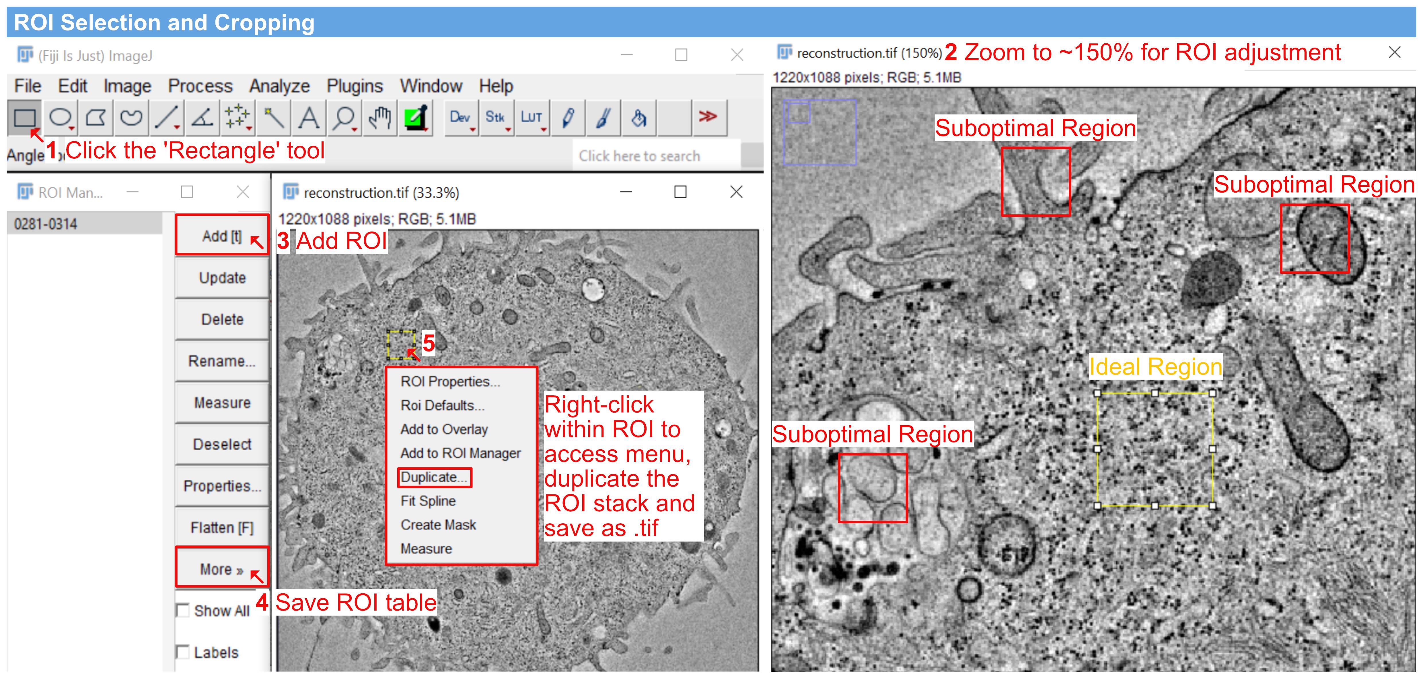
Figure 5. ROI selection and cropping in Fiji. Rectangle selection tool (1) with the view zoomed to approximately 150% for precise ROI adjustment (2). One ideal region and three suboptimal regions are indicated: the ideal region lies within the cell interior and contains predominantly ribosomes, whereas the suboptimal regions contain mitochondria, vesicles, or membrane-rich areas. Minor intrusions into the ROI are acceptable (see step C3). Adding the region in the ROI Manager (3) and saving the ROI table for reproducibility (4). Duplicating the selection and saving it as a .tif file (5).
D. Pixel-size setting, image inversion, denoising, and ribosome segmentation (arivis Pro 4.5)
Note: Segmentation is carried out in arivis Pro. Image loading, pixel-size setting, and the invert pipeline appear in Figures 6 and 7; denoising, Blob Finder, filtering, and export appear in Figure 8.
1. Load the dataset: Drag and drop the duplicated ROI selection indicated in step C5 into the arivis Pro workspace window to load the volume dataset (Figure 6).
Note: Each of the five cropped ROIs per tomogram is loaded and processed separately. Once the pipeline has been built (steps D3–7), it can be saved and reapplied to the remaining ROIs without reconfiguration.
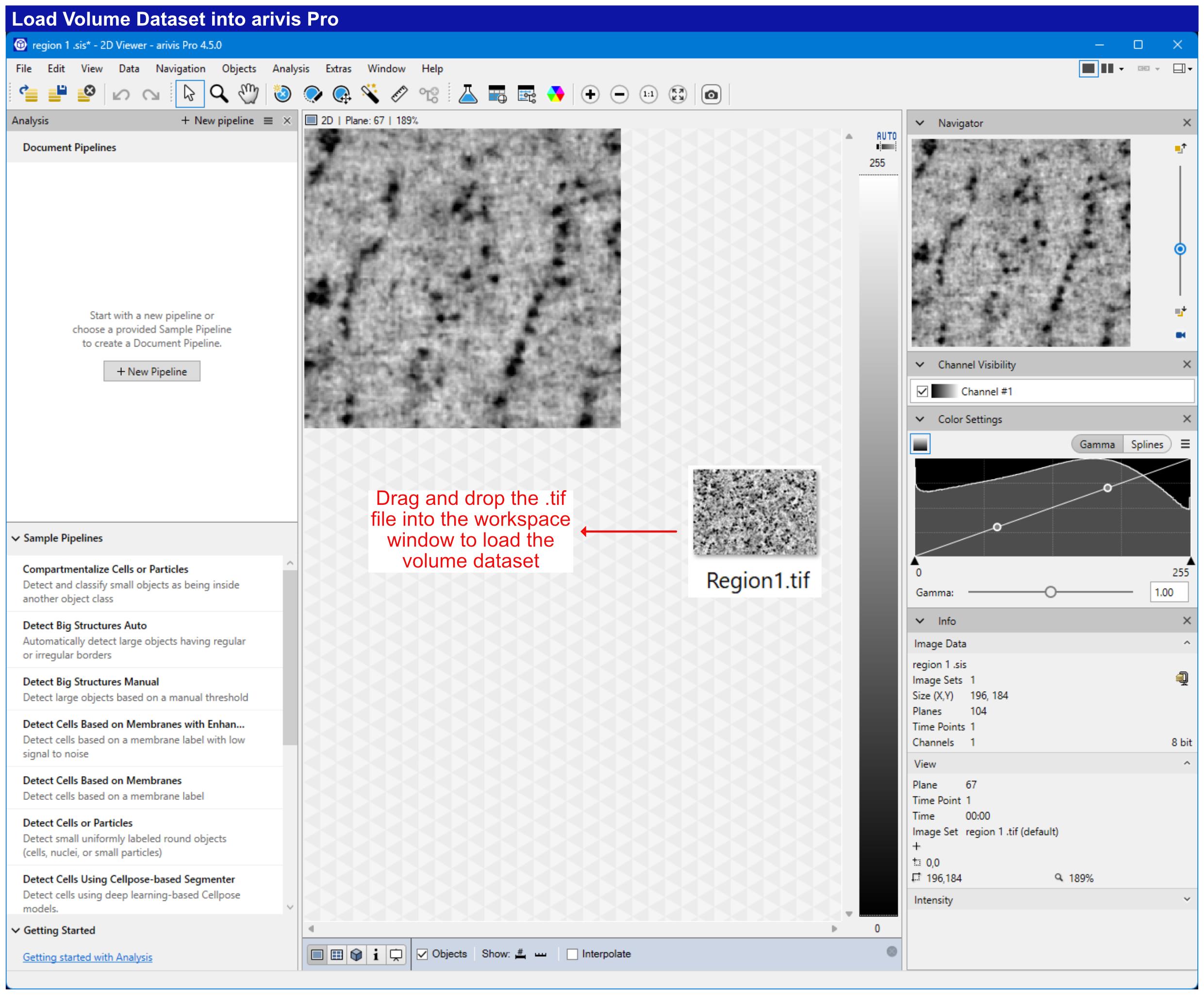
Figure 6. Loading the tomogram volume into arivis Pro. Drag-and-drop the cropped .tif ROI stack into the arivis Pro workspace to load the volume dataset.
2. Set the correct pixel size: In Fiji, open Image > Properties and note the Pixel width, Pixel height, and Voxel depth values (Figure 7A). In arivis Pro, open Data > Pixel Size… (Ctrl+Shift+P), enter the same X, Y, and Z values in the Change Pixel Size dialog, and click Change Pixel Size (Figure 7B). In our case, the voxel size is 0.002572 μm (2.572 nm) isotropic in X, Y, and Z.
3. Initialize a new pipeline and invert the image. Create a new pipeline and verify the Input ROI settings as Custom ROI, All Planes, and 100% Scaling (Figure 7C). Set the output storage to New Document and specify the output file path (Figure 7D). Add the Invert operation so that the stained ribosomes appear as local maxima (Figure 7E).
4. Denoise: In the Result Storages panel, change the Segments dropdown from Source Image Set to Result Image Set. Click + Add operation…, search for “denoising”, and add Image processing > Enhancements > Denoising (Figure 8A). Set Method to Median, Diameter to 7.72 nm, and Rank to 50%; then, click the Play/Start button (Figure 8B).
Note: The diameter of 7.72 nm corresponds to a 3 × 3 × 3 voxel median kernel at our voxel size of 2.572 nm. If your voxel size differs, set the diameter to three times your voxel size to preserve the same kernel width; a larger kernel will blur adjacent ribosomes together, and a smaller one will leave residual noise that the Blob Finder may detect as objects.
5. Blob Finder segmentation: Add the Blob Finder operation, check Store all inputs, and ensure Blob Finder is selected (Figure 8C). Set Diameter to 30 nm, Probability threshold to 30%, and Split sensitivity to 70% (Figure 8D). Eukaryotic ribosomes have a reported diameter of 20–30 nm [20,21]. The Diameter parameter specifies the expected upper size of the objects to be detected, so it was set to 30 nm; smaller densities down to the resolution limit of the reconstruction are still detected, and implausibly small objects are removed later by the voxel-count thresholds (step D9).
Note: The probability threshold sets the minimum probability coefficient for a density to be accepted as an object; the value of 30% is permissive, with false positives later removed by the voxel-count filters. The split sensitivity controls how touching objects are separated (higher values split more objects, lower values fuse more); the value of 70% ensures that densely packed, touching ribosomes are counted individually.
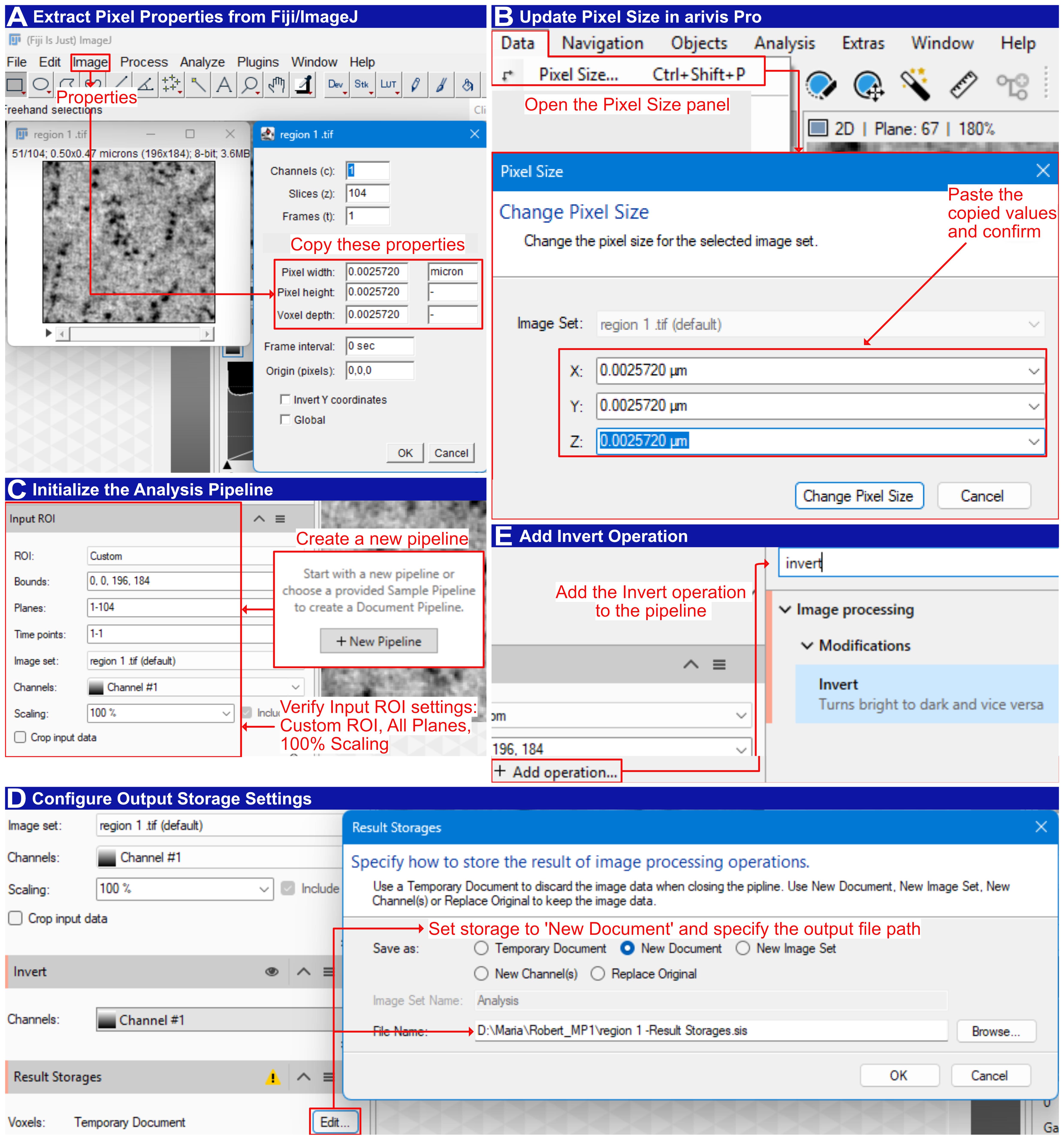
Figure 7. Pixel-size transfer and pipeline initialization in arivis Pro. (A) Extract pixel properties from Fiji/ImageJ: open the Properties dialog and copy the pixel width, pixel height, and voxel depth values (0.0025720 µm, i.e., 2.572 nm). (B) Update the pixel size in arivis Pro: open the Pixel Size panel, then paste the copied X, Y, and Z values into the Change Pixel Size dialog and confirm. (C) Initialize the analysis pipeline: create a new pipeline and verify the Input ROI settings (Custom ROI; all planes, 1–104; 100% scaling). (D) Configure output storage settings: in Result Storages, set Save as to New Document and specify the output file path. (E) Add the Invert operation to the pipeline so that stained ribosomes appear as local maxima.
6. Touching Edge Filter: Click + Add operation…, search for “touching edge filter”, and add Use objects > Special > Touching Edge Filter (Figure 8E). Set Input to Blob Finder, check the Z Top and Z Bottom boxes under Edges to handle, and change the Outputs display from red to multicolor (Figure 8F). In the Store Objects section, ensure Touching Edge Filter is checked.
Note: This filter removes found objects depending on the selected parameters. In this case, Z Top and Z Bottom boxes were checked; therefore, all objects in the upper and lower Z planes are removed. The X and Y edges are left unchecked because the ROI is cropped from within the cytoplasm (step C3), and lateral truncation at the ROI boundary does not indicate a genuinely incomplete particle. By contrast, objects at the Z limits are truncated by the physical section surface, so their voxel counts would not reflect the true particle volume.
7. Object Feature Filter: Click + Add operation… and add the Object Feature Filter. Set Input to Touching Edge Filter, Is of type to Segment, and the condition to Count (Plane) > 1, and change Outputs from green to multicolor. In the Store Objects section, ensure Object Feature Filter is checked. This removes flat segments (Figure 8G).
Note: The condition Count (Plane) > 1 requires each retained object to span more than one Z-plane. A genuine ribosome of 20–30 nm diameter occupies roughly 8–12 planes at a voxel size of 2.572 nm, so single-plane detections are almost always noise or staining artifacts rather than particles.
8. Export: Open the Objects window, click Im/Export…, and select Export Objects (Figure 8H). Under Report, choose Single table. Click Select… beside Features and check the six features required for the downstream quantification: Volume, VoxelCount, and RelativeVolume under Volume, and First, Last, and Count under Plane. Set Objects to All, specify the output path under Save As, and click Export to write the .xlsx file.
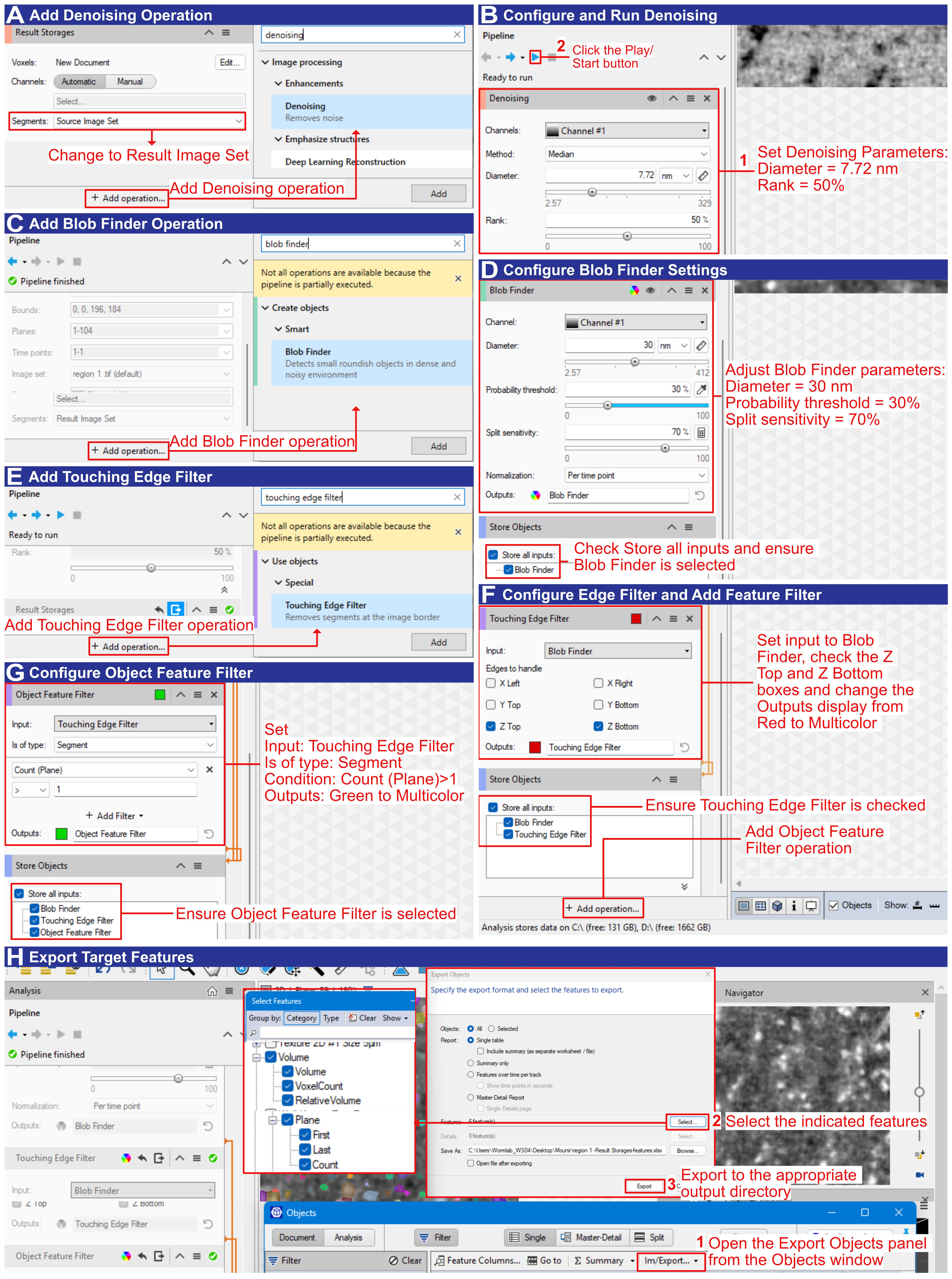
Figure 8. Semi-automated ribosome segmentation in arivis Pro. (A) Swapping to the Result Image Set and adding the Denoising operation. (B) Configuring and running denoising (Median filter; Diameter 7.72 nm; Rank 50%), then clicking the Play/Start button. (C) Adding the Blob Finder operation, checking Store all inputs, and ensuring Blob Finder is selected. (D) Configuring Blob Finder settings (Diameter 30 nm; Probability threshold 30%; Split sensitivity 70%). (E–F) Adding and configuring the Touching Edge Filter, setting the input to Blob Finder, checking the Z Top and Z Bottom boxes, and changing the Outputs display from Red to Multicolor. (G) Adding and configuring the Object Feature Filter (Input: Touching Edge Filter; Is of type: Segment; Condition: Count (Plane) > 1; Outputs: Green to Multicolor) to remove flat segments. (H) Opening the Export Objects panel from the Objects window and selecting the indicated features. Exporting the target features to the appropriate output directory as an .xlsx file.
9. Voxel-count thresholds: Exclude objects larger than 830 voxels in the exported .xlsx files. This upper limit is derived from the volume of a 30-nm-diameter sphere [4/3 × π × (15 nm)3 ≈ 14,137 nm3] divided by the voxel volume (2.5723 ≈ 17 nm3), giving ≈ 832 voxels, rounded down to 830 (Figure 9A). Conversely, a theoretical lower limit of 150 voxels (based on a 20 nm sphere diameter corrected for shrinkage: 4/3 × π × (10 nm)3 / 1.575 ≈ 2,660 nm3 ≈ 156 voxels, rounded down to 150 voxels) was found to exclude structures that are clearly identifiable as ribosomes in 2D views. For a general idea about potential ribosome structures in 2D and 3D views and the impact of thresholding, see Supplemental Figure S3 in the original paper [1]. Therefore, apply the empirically determined lower thresholds of 25, 50, and 100 voxels and report the resulting ribosome numbers for each threshold (Figure 9A). See Result interpretation for more details, and Troubleshooting (Problems 3–5) for addressing false positives, over-splitting, and large aggregates.
Notes:
1. In our dataset, applying the theoretical lower voxel limit excluded many structures identifiable as ribosomes from our segmentation. This might not be the case in your tomograms. We encourage readers to first test the theoretical limits, evaluate the outcome in 2D and 3D views, and then test several empirical thresholds. In our experience, there is no single optimal threshold, and multiple should always be compared. It is crucial that the final number of ribosomes lies in the same orders of magnitude, and that the numerical variations are reported.
2. If your voxel size differs from ours, the volume of a single voxel must be recalculated, along with the corresponding voxel-count thresholds required to account for ribosomes in the 20–30 nm size range.
E. Quantification, shrinkage correction, and cell-volume normalization
Note: Quantification is performed in a spreadsheet and is summarized in Figure 9. Figure 9A shows the voxel-count filtering of the exported object table; Figure 9B shows the subsequent calculation of ribosome concentration and the shrinkage correction, with two worked examples.
1. Extract ROI dimensions: Extract the dimensions of the cropped ROI regions (X, Y, Z) in pixels (px) from Fiji or arivis Pro, along with their corresponding number of objects (ribosome counts), and enter them into a new table (Figure 9B, columns for dimensions of the ROI (px) and ribosome count).
2. Calculate ROI volume: Calculate the volume of the ROI cropped region in cubic micrometers (μm3) by multiplying the dimensions by their voxel size (Figure 9B).
3. Calculate ribosome concentration: Calculate the ribosome concentration per cubic micrometer in the cropped ROI region by dividing the ribosome count by the volume (Figure 9B).
4. Apply the shrinkage correction: Calculate the shrinkage-corrected ribosome concentration by dividing the ribosome concentration by the shrinkage factor (Figure 9B).
Notes:
1. The shrinkage factor is determined as the ratio of the reconstructed section thickness (measured in the final tomogram) to the nominal thickness set on the ultramicrotome. Because resin sections collapse in the electron beam during acquisition [22–24], this factor is specific to the resin and freeze-substitution protocol used; the value of 1.575 reported here was determined from 77 Epon/Araldite datasets and must be recomputed for other resins.
2. Dividing the concentration by the shrinkage factor is equivalent to correcting the Z dimension of the ROI volume; the factor is not applied to X or Y.
5. Average across ROIs: Apply steps E1–4 to each cropped ROI region of each sample and average the values to obtain the shrinkage-corrected mean ribosome concentration per cubic micrometer for that specific sample.
Note: Please check Supplemental Table (Data 4) in the original paper for a global overview of how data is structured [1].
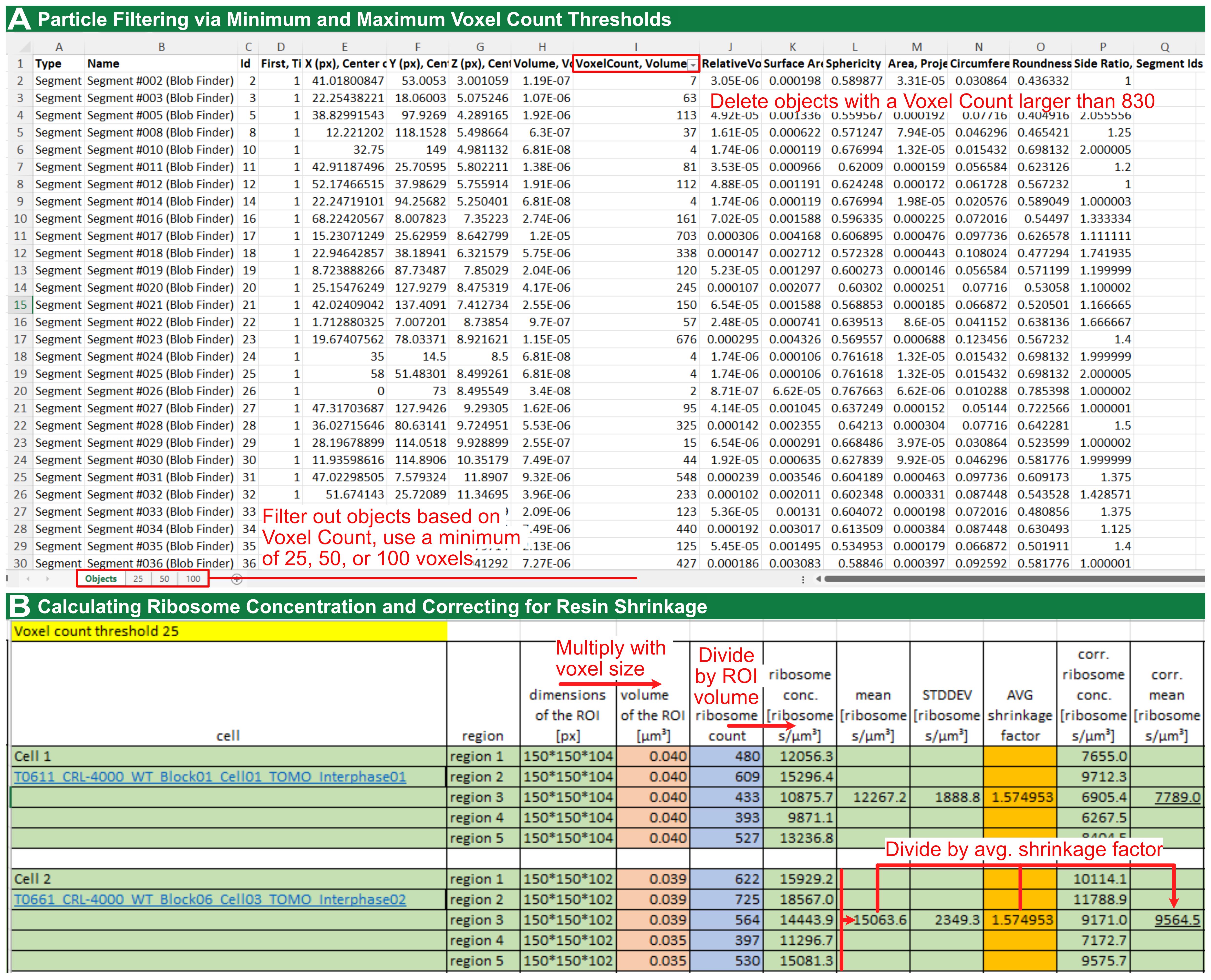
Figure 9. Quantification of ribosome number after segmentation in arivis Pro. (A) Deleting objects with a voxel count larger than 830 in the .xlsx file, followed by thresholding using a minimum of 25, 50, and 100 voxels. (B) Calculating ribosomes per cubic micrometer in the available volumes, followed by application of the resin-specific shrinkage factor.
6. Measure the cytoplasmic volume:
a. To determine the number of ribosomes per cell, measure the cytoplasmic volume using confocal microscopy. For this measurement only, use rounded cells up to passage number 4 and detach them using 0.25% trypsin.
b. Stain the cells with MemBrite Fix 543/560 for the plasma membrane and DAPI for the nucleus, then fix them in ice-cold methanol.
c. Locate the cells through the ocular lenses before switching to laser scanning for image acquisition.
d. Record images on a confocal microscope (Leica TCS SP5) equipped with a 40×/1.25 HCX PL APO lambda blue oil objective. For DAPI, illuminate at 405 nm and collect emission between 415 and 480 nm; for MemBrite, illuminate at 543 nm and collect emission between 550 and 700 nm.
e. Acquire images in an XY scan field of 512 × 512 pixels with a Z-dimension sufficient to capture the entire cell volume (40–50 μm).
f. In arivis Pro, segment the whole cell from the MemBrite channel and the nucleus from the DAPI channel as two separate objects, and read their volumes from the object table using the same Volume feature applied to the ribosome segments.
g. Estimate the cytoplasmic volume of each cell by subtracting its own nuclear volume from its whole-cell volume.
h. Additionally, subtract 10% of the total cell volume to account for non-ribosomal compartments. This allowance is based on the reported mitochondrial volume fraction of approximately 8% in retinal pigment epithelium [25], with a further ~2% allowed for other organelles; it is an approximation and should be re-determined for other cell types (see note below).
Notes:
1. Methanol fixation at low concentrations (12.5%–25%) causes measurable cell shrinkage, whereas at 50% and above, the projected cell area is statistically indistinguishable from untreated controls, which the authors attribute to the fixative effect of methanol at higher concentrations [26]; we therefore use undiluted ice-cold methanol. Confocal Z-sectioning with a fluorescent boundary marker is an established approach for microscopy-based cell volume measurement [27].
2. When an oil-immersion objective is used with an aqueous sample, the nominal Z-step overestimates the true focal-plane shift by approximately n_sample/n_immersion. Readers may either apply this correction or use a water- or silicone-immersion objective to avoid it [27].
3. This conversion applies to isolated cultured cells only. For C. elegans tissues, ribosome densities per μm3 are reported without extrapolation to whole cells. The 10% organelle allowance is specific to RPE-1 cells and should be re-determined for other cell types.
7. Calculate ribosomes per cell. Multiply the shrinkage-corrected mean ribosome concentration from step E5 by the cytoplasmic volume from step E6. For our hTERT-RPE-1 data at a voxel-count threshold of 25, a mean density of 8,754 ± 1,644 ribosomes/μm3 and a mean cytoplasmic volume of 1,787.4 ± 769.8 μm3 give approximately 15.6 × 10⁶ ± 1.3 × 10⁶ ribosomes per cell, in agreement with the independent biochemical estimate of 18.7 × 10⁶ ± 4.4 × 10⁶ obtained by rRNA capillary electrophoresis (see Validation of protocol) [1].
Note: The ribosome density per μm3 is the primary and most robust output of this protocol. The per-cell number is a derived estimate that inherits the larger uncertainty of the cytoplasmic volume measurement (coefficient of variation ≈ 43% in our data, compared with ≈ 19% for the density), reflecting genuine cell-to-cell size variation in an unsynchronized population. We recommend reporting the density alongside any per-cell figure so that the extrapolation step remains transparent.
Result interpretation
The primary and most robust output of this pipeline is the shrinkage-corrected ribosome density (ribosomes per μm3), obtained by dividing the object count in each cropped sub-volume by the sub-volume and by the resin-specific shrinkage factor. Where a whole-cell figure is required, this density is multiplied by the cytoplasmic volume; that per-cell number is a derived estimate and carries the larger uncertainty, because the cytoplasmic volume varies considerably between cells (coefficient of variation ≈ 43% in our data, compared with ≈ 19% for the density). We therefore recommend reporting the density alongside any per-cell figure, so that the extrapolation step remains transparent. When interpreting these values, several methodological considerations must be taken into account.
The reported ribosome number predictably depends strongly on the chosen voxel-count threshold. In hTERT-RPE-1 cells, densities decreased from 8,754 ± 1,644 to 5,505 ± 1,505 ribosomes per μm3 as the lower threshold was increased from 25 to 100 [1]. A lower threshold captures more ribosome-like structures in 2D view but also admits smaller globular objects in 3D view, which might be unassembled subunits, stained non-ribosomal proteins (proteasomes and major vault proteins), or glycogen granules; conversely, a higher threshold is more conservative. Reporting several thresholds is not a statistical sensitivity analysis, and the spread between them is not a readout of false positives versus false negatives: neither can be counted, because heavy-metal staining is nonspecific, and resin-embedded material provides no independent ground truth at the level of the single particle. What the threshold series provides is a bracket on the estimate. The lowest threshold gives an upper estimate that admits some non-ribosomal densities, and the highest gives a lower estimate that excludes some genuine ribosomes. The requirement is therefore that the resulting counts agree in order of magnitude and that the variation between them is reported, so that a reader can judge how much of the result depends on this choice. For this reason, we recommend reporting the ribosome number from at least three voxel-count thresholds after evaluating the lower theoretical voxel-count threshold. In our own data, the value at threshold 25 is treated as an upper estimate, and objects between approximately 25 and 830 voxels are considered indicative of ribosomes (Supplemental Figure S3 in [1]).
A useful quality-control step is to verify the whole-cell estimate by performing an independent biochemical measurement using the Bioanalyzer 2100 equipped with the RNA 6000 Nano Kit (Agilent) according to the manufacturer’s instructions. In the validation study, the electron tomography estimate of (15.6 ± 1.3) × 106 ribosomes per hTERT-RPE-1 cell at threshold 25 agreed with the (18.7 ± 4.4) × 106 ribosomes obtained by rRNA capillary electrophoresis [1], a difference of approximately 17%, with overlapping uncertainty intervals. Because the two routes share no common source of error (one depends on segmentation thresholds, the shrinkage correction, and confocal volumetry; the other on RNA extraction efficiency and rRNA-to-ribosome stoichiometry), their agreement constitutes an independent test rather than an internal consistency check, and indicates that the segmentation parameters, shrinkage factor, and thresholding are adequate for ribosome number estimation in cellular sub-volumes.
The segmented ribosome volume is consistently smaller than the theoretical value. Three factors contribute: shrinkage during sample preparation, beam-induced collapse of the resin section during acquisition, and the fact that ribosomes are not truly spherical, whereas the theoretical volume is calculated for a sphere [1]. This is why it is essential to apply the resin-specific shrinkage factor and several voxel-count thresholds; without these, densities and per-cell counts are readily underestimated. If measured densities appear implausibly low, verify that the shrinkage factor was derived for the resin actually used and that it was applied to the derived ribosome concentration (step E4).
Densities are not expected to be uniform across cell types, and biologically meaningful differences can be resolved. In C. elegans, ribosome density varied by tissue, with the distal gonad (20,618 ± 3,566 per μm3 at threshold 25) exceeding the somatic vulva cells (11,599 ± 4,448) [1]. Depletion of RPOA-1, a core subunit of RNA polymerase I, by RNAi significantly reduced ribosome density in the distal gonad and pachytene region but not in vulva cells at threshold 25, consistent with the higher transcriptional and translational demand of the germline [1]. When comparing conditions, apply the same threshold and shrinkage factor throughout, and test differences with an appropriate statistical test such as Welch’s two-sided t-test.
Finally, because only small volumes selected for predominantly ribosomal content are sampled, the whole-cell extrapolation assumes that ribosome density in these regions represents the wider cytoplasm and that non-ribosomal compartments occupy approximately 10% of the cytoplasmic volume. If this fraction is underestimated, the per-cell count will be overestimated [1]. We therefore recommend that readers determine the organelle volume fraction for their own cell type rather than adopting our 10% allowance, which was derived for retinal pigment epithelium [25]. Reporting the number of tomograms and sub-volumes analyzed, together with the specific thresholds used, enables readers to evaluate the robustness of the results [1].
Validation of protocol
This protocol (or parts of it) has been used and validated in the following research article: El Hankouri et al. (2025). In situ quantification of ribosome number by electron tomography. Journal of Microscopy [1] (Figures 1–4; Supplemental Data S1–S8).
The protocol was validated on cultured hTERT-RPE-1 cells and on C. elegans tissues. For each condition, multiple tomograms were analyzed (Table 2), and five independent ROIs were segmented per tomogram to capture cytoplasmic heterogeneity [1]. Tomographically determined ribosome densities were compared with biochemical rRNA quantification by capillary electrophoresis, including only samples with an RNA integrity number (RIN) above 9, and with a genetic perturbation, rpoa-1(RNAi), as controls [1]. Statistical comparisons used Welch’s two-sided t-test in R version 4.4.1, run in RStudio [1]. Ribosome numbers were evaluated across voxel thresholds of 25, 50, and 100. These were divided by a laboratory- and resin-specific shrinkage factor of 1.575 and compared to the biochemical analyses to demonstrate robustness [1].
Segmentation of five cytoplasmic sub-volumes across six interphase hTERT-RPE-1 tomograms yielded mean ribosome densities of 8,754 ± 1,644, 7,282 ± 1,628, and 5,505 ± 1,505 ribosomes per μm3 at thresholds of 25, 50, and 100, respectively [1]. Combined with a confocal-measured cytoplasmic volume of 1,787.4 ± 769.8 μm3, this yielded 15.6 × 10⁶ ± 1.3 × 10⁶ ribosomes per cell at threshold 25, closely matching the biochemical estimate of 18.7 × 10⁶ ± 4.4 × 10⁶ ribosomes per cell [1]. For C. elegans control animals at threshold 25, the distal gonad contained 20,618 ± 3,566, the pachytene region 18,950 ± 5,931, and vulva cells 11,599 ± 4,448 ribosomes per μm3 [1]. After rpoa-1(RNAi), ribosome density was significantly reduced in the distal gonad and pachytene region but not in vulva cells at threshold 25 [1].
Comparing the control versus rpoa-1(RNAi) groups, the distal gonad and pachytene region differed significantly across all thresholds, whereas vulval cells showed no significant difference at threshold 25 but reached statistical significance at thresholds 50 and 100 [1]. Comprehensive dataset-specific values and corresponding p-values can be found in Supplementary Data S4, S7, and S8 of the primary study [1].
Table 2. Validation data from El Hankouri et al. (2025) [1]. Values are mean ± SD ribosomes per μm3. n.a., not applicable (no comparison performed).
| Sample or condition | Tomograms (n) | ROIs per tomogram | Threshold 25 | Threshold 50 | Threshold 100 | Statistical test |
|---|---|---|---|---|---|---|
| hTERT-RPE-1, interphase | 6 | 5 | 8,754 ± 1,644 | 7,282 ± 1,628 | 5,505 ± 1,505 | n.a. |
| C. elegans distal gonad, control | 4 | 5 | 20,618 ± 3,566 | 15,198 ± 2,914 | 8,626 ± 2,202 | n.a. |
| C. elegans pachytene, control | 4 | 5 | 18,950 ± 5,931 | 13,283 ± 4,156 | 6,873 ± 1,895 | n.a. |
| C. elegans vulva, control | 4 | 5 | 11,599 ± 4,448 | 8,958 ± 3,077 | 5,472 ± 1,776 | n.a. |
| C. elegans distal gonad, rpoa-1(RNAi) | 4 | 5 | 12,817 ± 4,956 | 9,485 ± 3,507 | 5,312 ± 1,859 | Welch’s two-sided t-test |
| C. elegans pachytene, rpoa-1(RNAi) | 3 | 5 | 12,984 ± 4,432 | 9,029 ± 3,855 | 4,311 ± 2,224 | Welch’s two-sided t-test |
C. elegans vulva, rpoa-1(RNAi) | 3 | 5 | 9,089 ± 5,448 | 5,508 ± 3,294 | 2,708 ± 1,615 | Welch’s two-sided t-test |
General notes and troubleshooting
General notes
1. Record all parameters, including the HPF settings, AFS system program, resin recipe, nominal section thickness, TEM voltage, magnification, pixel size, IMOD and SerialEM parameters, and every arivis Pro segmentation value [1].
2. Acquire at least three tomograms per condition and crop five cytoplasmic ROIs per tomogram that contain predominantly ribosomes (see step C3 for selection criteria and acceptable intrusions) [1].
3. Compute a resin-specific shrinkage factor as the ratio of reconstructed to the nominal section thickness and apply it to the derived ribosome concentration (equivalently, to the Z dimension of the ROI volume). The Epon/Araldite shrinkage correction factor used here is 1.575 based on 77 stitched datasets, though this value may not apply to other resin formulations
[1,22–24].
4. Report at least three empirical thresholds (e.g., 25, 50 and 100) and justify the final choice, noting that a theoretical lower limit of 150 voxels excluded structures identifiable as ribosomes [1].
5. Corroborate imaging counts, where possible, with biochemical rRNA measurements and a biological perturbation such as rpoa-1(RNAi) [1].
6. Harvest cells for HPF by mitotic shake-off rather than trypsin, since trypsin-EDTA induces ribosome clustering that would bias density measurements [16]. Trypsin (0.25%) is used only for the confocal cell-volume measurement, where redistribution of ribosomes does not affect the geometric quantity being measured.
Troubleshooting
Problem 1: Variation of thickness within ribbons of serial sections for electron tomography.
Possible cause: Resin batch not hard enough. Thermal fluctuations or vibrations occurring during ultramicrotomy.
Solution: Do not use expired epoxy resin ingredients; prepare a fresh batch of resin. Also, monitor the section’s interference colors while sectioning (see Figure 1). Exclude sections that are too thick (which yield poor contrast) or too thin (which reduce tomographic volume) before data acquisition.
Problem 2: Poor ribosome contrast.
Possible cause: Insufficient heavy-metal staining.
Solution: Verify the FS protocol and AFS in-chamber temperatures, adjust post-staining times, and confirm graded infiltration [1,8].
Problem 3: High false-positive count.
Possible cause: Low probability threshold or inadequate denoising.
Solution: Raise the Blob Finder probability threshold, increase denoising, or raise the lower voxel threshold, then inspect the overlay [1].
Problem 4: Over-segmentation (excessive splitting) of ribosomes.
Possible cause: Split sensitivity threshold is set too high.
Solution: Reduce the split sensitivity parameter and slightly increase the median-filter diameter [1].
Problem 5: Large aggregates counted as ribosomes.
Possible cause: Upper voxel limit not enforced or bad cryo-preservation.
Solution: Exclude objects larger than 830 voxels and apply the Touching Edge and Object Feature filters [1]. If the sample is suffering from inadequate cryo-fixation (protein aggregation due to formation of hexagonal ice), exclude the tomogram from analysis.
Problem 6: Inconsistent ribosome counts between batches.
Possible cause: Differences in shrinkage rates, staining, or imaging settings.
Solution: Compute a batch-specific shrinkage factor, standardize acquisition, and include calibration samples, such as 20 nm or 30 nm gold beads on empty resin as a size standard [1].
Problem 7: Combine or Matchorwarp step fails in IMOD.
Possible cause: Alignment or stitching error.
Solution: Right-click the interface and select Show Log. Scroll to the bottom of the log to locate the specific error message; Etomo dynamically prints a direct parameter recommendation in the text based on the specific failure (e.g., suggesting a specific increase to the maximum residual or warp limit). Enter this newly recommended value into the corresponding field on the Initial Match or Final Match tab and re-run the step [1].
Supplementary information
The following supporting information can be used to replicate the analysis:
Dataset S1. OMERO access for all used datasets: https://omero.med.tu-dresden.de/webclient/?show=project-1303 (6 hTERT-RPE-1 tomograms, 22 C. elegans tomograms, and 2 overviews; see Table 1 from [1]).
Acknowledgments
Funding: Research in the Müller-Reichert lab is supported by grants from the Deutsche Forschungsgemeinschaft (DFG 258577783 and 282354882) to T.M.R. The Müller-Reichert laboratory also acknowledges support from the CCBx program (SF 1157392) of the Center for Computational Biology of the Flatiron Institute (NY, USA).
This protocol was described and validated in El Hankouri et al. (2025), Journal of Microscopy, DOI: 10.1111/jmi.13380 [1].
The sample preparation steps are adapted from our protocols for C. elegans [7] and for mammalian cells on sapphire discs [8]. We thank Silke Tulok and Dr. Anja Nobst (Core Facility Cellular Imaging, Faculty of Medicine Carl Gustav Carus, TU Dresden) for support in light microscopy and OMERO data management; Chukwuebuka William Okafornta for assistance with worm handling; and the EM facility at MPI-CBG, Dresden, for support in electron tomography. Some strains were provided by the CGC, which is funded by NIH Office of Research Infrastructure Programs (P40 OD010440).
Author contributions
Conceptualization, G.F. and T.M.R.; Investigation, M.E.H., A.P., and G.F.; Formal analysis, M.E.H., A.P., and G.F.; Software and pipeline, M.E.H., A.P., and G.F.; Writing—Original Draft, G.F.; Writing—Review and Editing, all authors; Supervision, G.F. and T.M.R.; Funding acquisition, T.M.R.
Competing interests
The authors declare no conflicts of interest. In particular, the authors have no financial or non-financial relationship with the manufacturer of arivis Pro or any other vendor whose products are named in this protocol.
Ethical considerations
This study used the invertebrate model system, Caenorhabditis elegans, and an established immortalized human cell line, hTERT-RPE-1; ATCC CRL-4000. Neither system requires ethics committee approval or informed consent, as no vertebrate animals or identifiable human subjects were involved. Where applicable, reporting follows the ARRIVE guidelines.
References
- El Hankouri, M., Nousch, M., Poddar, A., Müller‐Reichert, T. and Fabig, G. (2025). In situ quantification of ribosome number by electron tomography. J Microsc. 299(3), 212–227. https://doi.org/10.1111/jmi.13380
- Ortiz, J. O., Förster, F., Kürner, J., Linaroudis, A. A. and Baumeister, W. (2006). Mapping 70S ribosomes in intact cells by cryoelectron tomography and pattern recognition. J Struct Biol. 156(2): 334–341. https://doi.org/10.1016/j.jsb.2006.04.014
- Mahamid, J., Pfeffer, S., Schaffer, M., Villa, E., Danev, R., Kuhn Cuellar, L., Förster, F., Hyman, A. A., Plitzko, J. M., Baumeister, W., et al. (2016). Visualizing the molecular sociology at the HeLa cell nuclear periphery. Science. 351(6276): 969–972. https://doi.org/10.1126/science.aad8857
- Schaffer, M., Pfeffer, S., Mahamid, J., Kleindiek, S., Laugks, T., Albert, S., Engel, B. D., Rummel, A., Smith, A. J., Baumeister, W., et al. (2019). A cryo-FIB lift-out technique enables molecular-resolution cryo-ET within native Caenorhabditis elegans tissue. Nat Methods. 16(8): 757–762. https://doi.org/10.1038/s41592-019-0497-5
- Albert, S., Wietrzynski, W., Lee, C. W., Schaffer, M., Beck, F., Schuller, J. M., Salomé, P. A., Plitzko, J. M., Baumeister, W., Engel, B. D., et al. (2019). Direct visualization of degradation microcompartments at the ER membrane. Proc Natl Acad Sci USA. 117(2): 1069–1080. https://doi.org/10.1073/pnas.1905641117
- Conway, W., Bobe, D., Zimyanin, V., Fabig, G., de Marco, A. and Redemann, S. (2026). Eg5 activity and density-driven bundling organize the human metaphase mitotic spindle independently of spindle bipolarity. bioRxiv. e699769. https://doi.org/10.64898/2026.01.16.699769
- Fabig, G., Schwarz, A., Striese, C., Laue, M. and Müller-Reichert, T. (2019). In situ analysis of male meiosis in C. elegans. Methods Cell Biol. 152: 119–134. https://doi.org/10.1016/bs.mcb.2019.03.013
- Kiewisz, R., Baum, D., Müller-Reichert, T. and Fabig, G. (2023). Serial-section Electron Tomography and Quantitative Analysis of Microtubule Organization in 3D-reconstructed Mitotic Spindles. Bio Protoc. 13(20): e4849. https://doi.org/10.21769/bioprotoc.4849
- Stiernagle T. (2006). Maintenance of C. elegans. WormBook. 11:1–11. https://doi.org/10.1895/wormbook.1.101.1
- Bhattiprolu, S., Toor, M. and Soyer, S. (2026). ZEISS arivis Cloud: a cloud-based platform for deep learning model training and scalable bioimage analysis. bioRxiv. e743540. https://doi.org/10.64898/2026.08.07.743540
- Kremer, J. R., Mastronarde, D. N. and McIntosh, J. (1996). Computer Visualization of Three-Dimensional Image Data Using IMOD. J Struct Biol. 116(1): 71–76. https://doi.org/10.1006/jsbi.1996.0013
- Mastronarde, D. N. and Held, S. R. (2017). Automated tilt series alignment and tomographic reconstruction in IMOD. J Struct Biol. 197(2): 102–113. https://doi.org/10.1016/j.jsb.2016.07.011
- Mastronarde, D. N. (2003). SerialEM: A Program for Automated Tilt Series Acquisition on Tecnai Microscopes Using Prediction of Specimen Position. Microsc Microanal. 9: 1182–1183. https://doi.org/10.1017/s1431927603445911
- Mastronarde, D. N. (2005). Automated electron microscope tomography using robust prediction of specimen movements. J Struct Biol. 152(1): 36–51. https://doi.org/10.1016/j.jsb.2005.07.007
- Schindelin, J., Arganda-Carreras, I., Frise, E., Kaynig, V., Longair, M., Pietzsch, T., Preibisch, S., Rueden, C., Saalfeld, S., Schmid, B., et al. (2012). Fiji: an open-source platform for biological-image analysis. Nat Methods. 9(7): 676–682. https://doi.org/10.1038/nmeth.2019
- Furcht, L. and Wendelschafer-Crabb, G. (1978). Trypsin-induced coordinate alterations in cell shape, cytoskeleton, and intrinsic membrane structure of contact-inhibited cells. Exp Cell Res. 114(1): 1–14. https://doi.org/10.1016/0014-4827(78)90029-0
- Fire, A., Xu, S., Montgomery, M. K., Kostas, S. A., Driver, S. E. and Mello, C. C. (1998). Potent and specific genetic interference by double-stranded RNA in Caenorhabditis elegans. Nature. 391(6669): 806–811. https://doi.org/10.1038/35888
- Hammell, C. M. and Hannon, G. J. (2012). Inducing RNAi in C. elegans by Feeding with dsRNA-expressing E. coli. Cold Spring Harb Protoc. 2012(12): pdb.prot072348. https://doi.org/10.1101/pdb.prot072348
- Müller‐Reichert, T., Hohenberg, H., O'Toole, E. T. and Mcdonald, K. (2003). Cryoimmobilization and three‐dimensional visualization of C. elegans ultrastructure. J Microsc. 212(1): 71–80. https://doi.org/10.1046/j.1365-2818.2003.01250.x
- COX, R. and ARNSTEIN, H. (1963). THE ISOLATION, CHARACTERIZATION AND ACID-BASE PROPERTIES OF RIBONUCLEIC ACID FROM RABBIT-RETICULOCYTE RIBOSOMES. Biochem J. 89(3): 574–584. https://doi.org/10.1042/bj0890574
- Yi, X., Verbeke, E. J., Chang, Y., Dickinson, D. J. and Taylor, D. W. (2019). Electron microscopy snapshots of single particles from single cells. J Biol Chem. 294(5): 1602–1608. https://doi.org/10.1074/jbc.ra118.006686
- Gusnard, D. and Kirschner, R. H. (1977). Cell and organelle shrinkage during preparation for scanning electron microscopy: effects of fixation, dehydration and critical point drying. J Microsc. 110(1): 51–57. https://doi.org/10.1111/j.1365-2818.1977.tb00012.x
- Luther, P.K. (2007). Sample Shrinkage and Radiation Damage of Plastic Sections. In: Frank, J. (eds) Electron Tomography. Springer, New York, NY. https://doi.org/10.1007/978-0-387-69008-7_2
- Kizilyaprak, C., Longo, G., Daraspe, J. and Humbel, B. M. (2015). Investigation of resins suitable for the preparation of biological sample for 3-D electron microscopy. J Struct Biol. 189(2): 135–146. https://doi.org/10.1016/j.jsb.2014.10.009
- Pollreisz, A., Neschi, M., Sloan, K. R., Pircher, M., Mittermueller, T., Dacey, D. M., Schmidt-Erfurth, U. and Curcio, C. A. (2020). Atlas of Human Retinal Pigment Epithelium Organelles Significant for Clinical Imaging. Invest Ophthalmol Vis Sci. 61(8): 13. https://doi.org/10.1167/iovs.61.8.13
- Wang, Y., Yang, Y., Wang, D., Ouyang, L., Zhang, Y., Zhao, J. and Wang, X. (2013). Morphological Measurement of Living Cells in Methanol with Digital Holographic Microscopy. Comput Math Methods Med. 2013: 1–7. https://doi.org/10.1155/2013/715843
- Model, M. A. (2018). Methods for cell volume measurement. Cytometry. Cytom J Int Soc Anal Cytol. 93(3): 281–296. https://doi.org/10.1002/cyto.a.23152
Article Information
Publication history
Received: Jul 25, 2026
Accepted: Oct 7, 2026
Available online: Oct 22, 2026
Published: Nov 20, 2026
Copyright
© 2026 The Author(s); This is an open access article under the CC BY-NC license (https://creativecommons.org/licenses/by-nc/4.0/).
How to cite
El Hankouri, M., Poddar, A., Müller-Reichert, T. and Fabig, G. (2026). Semi-Automated Workflow for Segmenting and Quantifying Ribosomes in Electron Tomograms of High-Pressure Frozen and Resin-Embedded Samples. Bio-protocol 16(22): e5866. DOI: 10.21769/BioProtoc.5866.

 Download Citation in RIS Format
Do you have any questions about this protocol?
Post your question to gather feedback from the community. We will also invite the authors of this article to respond.
 Post a Question


