


- Protocols

- Articles and Issues
- For Authors
- About
- Become a Reviewer


Digital Quantification of Membrane DAB Immunohistochemical Staining in FFPE Cervical Cancer Tissues Using an Open-Source CellProfiler Pipeline


(*contributed equally to this work) Published: Vol 16, Iss 18, Sep 20, 2026 DOI: 10.21769/BioProtoc.5817 Views: 791
Reviewed by: Minal EngavaleAnonymous reviewer(s)
 PDF
PDF  Ask a question

Protocol Collections
Comprehensive collections of detailed, peer-reviewed protocols focusing on specific topics




Related protocols

Abstract
Immunohistochemistry (IHC) is a highly specific and widely used laboratory technique for assessing protein localization and expression in tissue samples. Interpretation of 3,3’ diamino benzidine (DAB)-based IHC is often based on observer-dependent manual scoring or traditional imaging software, which may show variability in DAB staining quantification. Furthermore, conventional image analysis tools often face limitations in precisely defining cell boundaries and quantifying membrane-specific signals. In this study, we present a standardized image analysis workflow using CellProfiler, an open-source software for image analysis for the quantification of membrane staining intensity in IHC images captured from slides prepared using formalin-fixed paraffin-embedded (FFPE) human cervical cancer tissue sections. The image analysis workflow was demonstrated using ASCT2 (SLC1A5), a membrane-localized amino acid transporter, as a representative biomarker for membrane-associated protein expression. This protocol involves image preprocessing, object identification, segmentation, and intensity measurement modules to distinguish cell membranes from cytoplasmic regions, enabling automated quantification of membrane intensity signals. The CellProfiler pipeline demonstrated improved accuracy in cell boundary identification and quantification of membrane-specific staining intensity. This is a rapid quantification process, since processing of each image only takes a few seconds; therefore, the analysis for 100 images can be performed within 10–15 min. This segmentation and quantification strategy is applicable to other membrane-based biomarkers after appropriate optimization of segmentation parameters. Following further minor modifications to the object identification modules, this pipeline can be used to detect and quantify cytoplasm- or nuclei-localized DAB-IHC markers across different tissue types. Overall, this protocol provides a standardized, user-friendly, and reproducible workflow for quantitative IHC image analysis that can be broadly applied to the study of protein biomarkers of different localizations, such as nuclei, cytoplasm, and cell membranes from different tissue types.
Key features
• Quantification of membrane-specific staining intensity in immunohistochemistry (IHC) images using a customized CellProfiler analysis pipeline.
• Accurate delineation of cell boundaries, allowing separation of membrane and cytoplasmic signal regions.
• Reproducible stepwise workflow adaptable to multiple tissue types and membrane protein biomarkers.
• Applicability to studies of membrane-localized biomarkers, such as ASCT2, in cancer research.
Keywords: Immunohistochemistry CellProfiler Imaging software
Image analysis
Membrane protein quantification
Cancer
Digital pathology
CellProfiler Imaging software
Image analysis
Membrane protein quantification
Cancer
Digital pathology
Background
Immunohistochemistry (IHC) is an important technique in histopathology for detecting the localization of specific proteins in formalin-fixed paraffin-embedded (FFPE) tissue sections. It enables the visualization of protein expression while preserving tissue architecture [1,2]. 3,3'-diaminobenzidine (DAB) is the most commonly used chromogenic substrate since it is stable and compatible with brightfield microscopy; also, it has the ability to produce a permanent brown precipitate at sites of antigen–antibody interaction [3]. Because of these advantages, DAB-based IHC has become an indispensable tool for routine diagnostics and in biomarker research [4]. However, the interpretation of DAB staining is often observer-dependent, relying on manual scoring systems (e.g., Q-score or H-score). This introduces inter-observer variability, thereby limiting reproducibility across studies and laboratories [5,6].
Recent advances in the domains of digital pathology and image analysis have overcome many limitations associated with manual assessment by enabling high-throughput quantification of immunohistochemical signals, thereby making the detection of signals very quick and accurate [7,8]. Open-source software such as CellProfiler provides a user-friendly interface for designing image analysis pipelines. It enables segmentation of cellular compartments and extraction of quantitative features from histological images, making it convenient for researchers to analyze images without requiring programming expertise [9,10]. These open-source tools are very useful as they eliminate the need for expensive proprietary software, also supporting reproducibility and transparent workflows.
In the context of DAB staining, due to the heterogeneity in staining intensity, the addition of counterstains such as hematoxylin, which causes difficulty in the separation of signals and variability in tissue morphology, makes it harder to accurately quantify signals [11–13]. Although color deconvolution methods can separate chromogenic signals [14], implementing these workflows in a standardized and reproducible manner remains a practical barrier for many laboratories. Furthermore, there is a growing need for standardized and accessible pipelines that can be readily adapted to different tissue types and biomarkers. To address these challenges, this protocol describes a simple and rapid pipeline for quantifying DAB-based IHC staining using CellProfiler, with minimal user intervention and no requirements for advanced computational expertise.
In this protocol, FFPE sections of human cervical cancer tissues were used to perform IHC using an antibody that targets ASCT2 (SLC1A5), which is a protein involved in the transport of glutamine, predominantly localized in the cell membrane. These slides were stained and imaged using a brightfield microscope. The primary focus of this protocol is the application of the pipeline created using CellProfiler to process the images taken after performing IHC, followed by data analysis steps.
The current protocol differs from image analysis protocols from previous studies, as these do not have a fixed pipeline to perform image processing and analysis after IHC. Furthermore, traditional imaging software, such as ImageJ and QuPath, could not provide accurate individual cell detection and membrane staining intensity quantification. Moreover, many workflows require manual region-of-interest selection, sequential processing steps, or macro scripting for high-throughput analysis. In contrast, CellProfiler provides a modular, pipeline-based workflow that enables automated batch processing, reproducible object identification, and quantitative extraction of multiple cellular features without requiring programming expertise. This protocol allows for relatively precise and efficient means of intensity quantification and further downstream analysis through the combination of software such as CellProfiler and Microsoft Excel. This allows for simplified image analysis across multiple tissue types and experimental groups. However, it is important to note that DAB chromogenic intensity, as measured here, is best suited to relative comparisons between samples processed, stained, and imaged under standardized conditions. It should not be interpreted as an absolute measure of protein abundance, since chromogenic intensity can be affected by variables such as antibody, incubation time, and section thickness that are not directly related to the target expression level.
Materials and reagents
Biological materials
The protocol was developed and validated using 4-μm-thick FFPE human cervical cancer tissue sections obtained from surgical specimens from cervical cancer patients undergoing treatment at SRIHER, following approval from the Institutional Ethics Committee (REF: IEC-NI/22/JUL/83/94). Tissue samples were fixed in 10% neutral buffered formalin for 48 h, processed according to standard histopathology procedures, and embedded in paraffin. Human cervical cancer specimens (n = 3 per condition) were stained with ASCT2 (SLC1A5) using DAB-based immunohistochemistry.
Reagents
1. Xylene (Merck, catalog number: IA51640305)
2. 100% isopropyl alcohol (IPA) (Qualigens, catalog number: Q26897)
3. Tris base (Himedia, catalog number: TC072)
4. EDTA (Himedia, catalog number: GRM1195-100G)
5. Sodium chloride (NaCl) (Himedia, catalog number: GRM031-500G)
6. Tween-20 (Himedia, catalog number: MB067-100ML)
7. Sodium bicarbonate (Himedia, catalog number: PCT1535-500g)
8. Hydrophobic barrier PAP pen (Sigma-Aldrich, catalog number: Z377821-1EA)
9. Mouse/Rabbit Polyvue HRP/DAB Detection System (for mouse and rabbit primary antibodies) (Diagnostic Biosystems, catalog number: PVP100D)
a. Tissue primer (10 mL)
b. Background blocker (10 mL)
c. PolyVue Plus mouse/rabbit enhancer (10 mL)
d. PolyVue Plus mouse/rabbit HRP label (10 mL)
e. Stable DAB/Plus buffer (15 mL)
f. Stable DAB/Plus chromogen (1 mL)
10. ASCT2/SLC1A5 rabbit mAb (Abclonal, catalog number: A23156)
11. Hematoxylin (Himedia, catalog number: S034-500ml)
12. Concentrated hydrochloric acid (HCl) (12 M solution) (Molychem, catalog number: 23540)
13. Dibutyl phthalate polystyrene xylene (DPX) mountant (Himedia, catalog number: 88147-500ml)
Note: The chemicals used in this protocol, namely 3,3'-diaminobenzidine (DAB) (CAS No. 7411-49-6), xylene (CAS No.1330-20-7), hydrochloric acid (HCl) (CAS No. 7647-01-0), and DPX mounting medium (CAS No. 130-12-2), are hazardous and should be handled in accordance with institutional chemical safety guidelines. Appropriate personal protective equipment (laboratory coat, gloves, and safety goggles) should be worn throughout the procedure. Procedures involving volatile or corrosive chemicals should be performed in a certified chemical fume hood where appropriate.
Detailed information regarding the hazards, safe handling procedures, storage conditions, first-aid measures, spill management, and disposal requirements for each chemical should be obtained from the manufacturer's Safety Data Sheet (SDS/MSDS) using the corresponding CAS number of the reagent being used. As SDS information may vary slightly between manufacturers and formulations, users should always consult the SDS supplied with their specific product before performing the protocol.
Chemical waste, including DAB, xylene, HCl, DPX, and contaminated consumables, should be collected and disposed of in accordance with institutional biosafety and hazardous chemical waste disposal regulations.
Solutions
1. Antigen retrieval buffer (see Recipes)
2. Wash buffer (1×) (see Recipes)
3. Sodium bicarbonate solution (see Recipes)
4. Acid alcohol solution (see Recipes)
Recipes
1. Antigen retrieval buffer
Add 1.214 g of Tris base (121.14 g/mol) and 0.372 g of EDTA (292.24 g/mol) to 800 mL of distilled water. Adjust the pH to 9.0 and make up to 1 L. Store at 4 °C for 1 month.
2. Wash buffer (1×)
Dissolve 2.42 g of Tris base and 8 g of NaCl (58.44 g/mol) in 800 mL of distilled water. Adjust the pH to 7.6 and make up to 1 L. Add 1 mL of Tween-20 to this solution. Store at 4 °C for 1 month.
3. Sodium bicarbonate solution
Dissolve 1 g of sodium bicarbonate (84.007 g/mol) in 50 mL of distilled water.
4. Acid alcohol solution
Add distilled water to 35 mL of 100% IPA to make it up to 50 mL. Mix 200 μL of concentrated HCl (12 M).
Laboratory supplies
1. Micropipette tips (10 μL, 200 μL, and 1 mL) (Tarsons, catalog numbers: 521000PP, 5210101P, 521020P)
2. 1.5 mL microcentrifuge tubes (Tarsons, catalog number: 5000010)
3. Parafilm M (Tarsons, catalog number: 380020)
4. Coplin jars
5. Humidifying chamber
6. Positively charged slides (PathnSitu, catalog number: PS011)
7. Coverslips (22 × 60 mm) (Blue Star)
8. Staining rack
Equipment
1. Brightfield microscope (Leica, model: DM 2000 LED) with LAS 4.5 software
2. Leica MC170 HD digital camera
3. Hot air oven (Equitron) for baking at 70 °C and for slide drying at 40 °C
4. Pressure cooker for antigen retrieval
5. Induction stove
Software and datasets
| Type | Software/dataset/resource | Version | Date | License | Operating system | Access |
|---|---|---|---|---|---|---|
| Software 1 | CellProfiler | 4.2.6 | 2023 | BSD 3-Clause License | macOS Ventura 13.2.1 and Windows 11 | Free |
| Software 2 | Microsoft Excel | Office 2019 | 2018 | Proprietary (Microsoft License) | macOS Ventura 13.2.1 and Windows 11 | Paid |
| Data | ASCT2 IHC images (Imaged from DAB-stained FFPE tissue slides) | - | - | Not publicly available |
Procedure
A. Immunohistochemistry (Day 1)
1. Bake the tissue slides in a hot air oven at 70 °C for 1 h to ensure that all the wax is melted.
2. Add xylene to two staining trays. Keep the slides in a slide staining rack and in the first xylene wash for 10 min. Then transfer the slide staining rack to the second xylene wash for another 10 min.
3. After draining the excess xylene, move the slides to a staining tray containing 100% IPA for 5 min. Repeat this twice.
4. Fill a Coplin jar with antigen retrieval buffer and place it into a pressure cooker until the retrieval buffer reaches boiling temperature.
5. Once the second IPA wash is done, keep the slides under running water for 5 min.
6. Transfer the slides into the pre-heated Coplin jar containing antigen retrieval buffer and place it inside the pressure cooker. Secure the pressure cooker lid and heat using an induction stove (1 kW) until full pressure is reached. Continue heating until two pressure-release whistles are generated.
7. Turn off the heat and allow the pressure cooker to cool naturally for 10–15 min until the pressure is fully released.
8. Dry the slides by dabbing around the tissue sample with tissue paper.
9. Mark the outer boundary of the sample using a hydrophobic PAP pen and add two drops of tissue primer to cover the whole tissue. Leave it undisturbed for 5 min.
10. Transfer the slides to wash buffer for 5 min.
11. Add background blocker to the tissue and leave undisturbed for 5 min.
12. Dilute the ASCT2 primary antibody to a 1:2,000 dilution using background blocker and add approximately 100 μL to the tissue section.
13. Place the slides in a humidifying chamber and incubate at 4 °C overnight.
B. Immunohistochemistry (Day 2)
1. Discard the primary antibody that remains on the slide and keep the slides in a Coplin jar containing wash buffer for a duration of 5 min.
2. Transfer the slides to a second Coplin jar containing fresh wash buffer and incubate for another 5 min. Then, remove the excess wash buffer.
3. Redraw the PAP boundary and place the slides back in the humidifying chamber.
4. Add 1–2 drops of the PolyVue Plus mouse/rabbit enhancer to each slide and incubate for 15 min at room temperature (20–25 °C).
5. Transfer the slides to wash buffer 1 for 5 min, followed by wash buffer 2 for 5 min.
6. Remove the excess buffer, add two drops of PolyVue Plus mouse/rabbit HRP label, and incubate for 15 min at room temperature (20–25 °C).
7. During this 15-min incubation, prepare the DAB solution by mixing 1 mL of Stable DAB/Plus buffer and two drops of Stable DAB/Plus chromogen with the lights turned off, as the DAB solution is light-sensitive.
8. Add 100 μL of the DAB solution to the slides and incubate at room temperature for 3 min.
9. After the 3-min incubation (when a brown color appears), immediately stop the reaction by rinsing the slides under running tap water for 2 min.
10. Transfer the slides into the Coplin jar containing hematoxylin for 3 min.
11. Place the slides under running water for 2 min; after, let them sit in a tray of water for 3 min.
12. Immerse the slides in a Coplin jar containing sodium bicarbonate for 30 s.
13. Place the slides under running water for 2 min and dip them in acid alcohol 1–2 times to remove excess hematoxylin staining, followed immediately by rinsing under running tap water for 2 min to remove excess stains.
14. Dry the slides using the hot air oven at 40 °C for 20 min.
15. Add two drops of DPX mountant to the coverslips and place the slides over the coverslips carefully to avoid air bubble formation.
16. Store the slides in the dark until they are dried and image using an upright brightfield microscope.
C. Image acquisition
1. Following IHC staining, image the slides using a Leica DM2000 brightfield microscope equipped with a Leica MC170 HD digital color camera. Perform image acquisition using Leica Application Suite (LAS) version 4.5.
2. Select representative fields containing tumor tissues under lower magnification and acquire the images used for the quantitative analysis at 40× magnification. Capture images using identical illumination and camera settings for all the slides to reduce inter-image variability.
3. Optimize camera settings before image acquisition and maintain them constant throughout imaging. In our work, images were acquired in 24-bit RGB color, with an exposure time of 40 ms, brightness set to 56%, and gamma set to 1.20, while the options Sharpen, Enhance Contrast, and High-Resolution Live were disabled to avoid image processing artifacts. Acquired images were reviewed using the LAS process module without altering original staining intensity. Each image was exported as an JPG file (1,024 × 768 pixels) with an embedded scale bar and saved for subsequent quantitative analysis using the CellProfiler pipeline.
D. CellProfiler pipeline
The analysis pipeline was constructed in CellProfiler. Default input modules include Images, Metadata, NamesAndTypes, and Groups. In this study, only the Images and NamesAndTypes modules were utilized, as the dataset did not require metadata extraction or grouping.
Step 1. Images module
1. Open CellProfiler and create a new project.
2. In the Images module, select the folder containing the acquired brightfield IHC Images (40× magnification, JPG format). Its purpose is to compile and load all raw image files that will be analyzed.
3. Select Images only under the Filter images? parameter. This ensures that only image files (e.g., .jpg, .png, .tif) are loaded and non-image files are excluded.
4. Click Apply filters to the file list to confirm selection.
5. Verify that the intended image(s) appear in the file list panel.
6. Enable Show files excluded by filters (optional) to confirm that no required images are accidentally filtered out.
Step 2. NamesAndTypes module
The NamesAndTypes module allows you to assign a meaningful name to each image by which other modules will refer to it.
1. Assign a name to All images.
2. Process as 3D: No.
3. Select the image type: Color image.
Note: Brightfield IHC DAB images contain RGB information (brown DAB chromogen and blue hematoxylin counterstain), so the image type is defined as color.
4. Name to assign these images: “Protein_Name”.
5. Set intensity range from Image metadata to preserve the original image scaling.
Step 3. Crop module
The Crop module (Figure 1) is used to remove unwanted regions of the image that may interfere with downstream analysis, such as scale bars or labels.
1. Add the Crop module in CellProfiler.
2. Select the input image: “Protein_Name” (from the NamesAndTypes module).
3. Name the output image “CropProtein”.
4. Select the cropping shape: “Rectangle”.
5. Select the cropping method: “Coordinates”. Cropping boundaries are defined manually using pixel coordinates.
6. Apply which cycle’s cropping pattern: “Every”. The same cropping coordinates are applied uniformly across all images in the dataset.
7. Set the left and right rectangle positions: “0 to end” (Absolute).
8. Set the top and bottom rectangle positions: “0 to 685” (Absolute).
9. Set “Remove empty rows and columns” to: “All”.
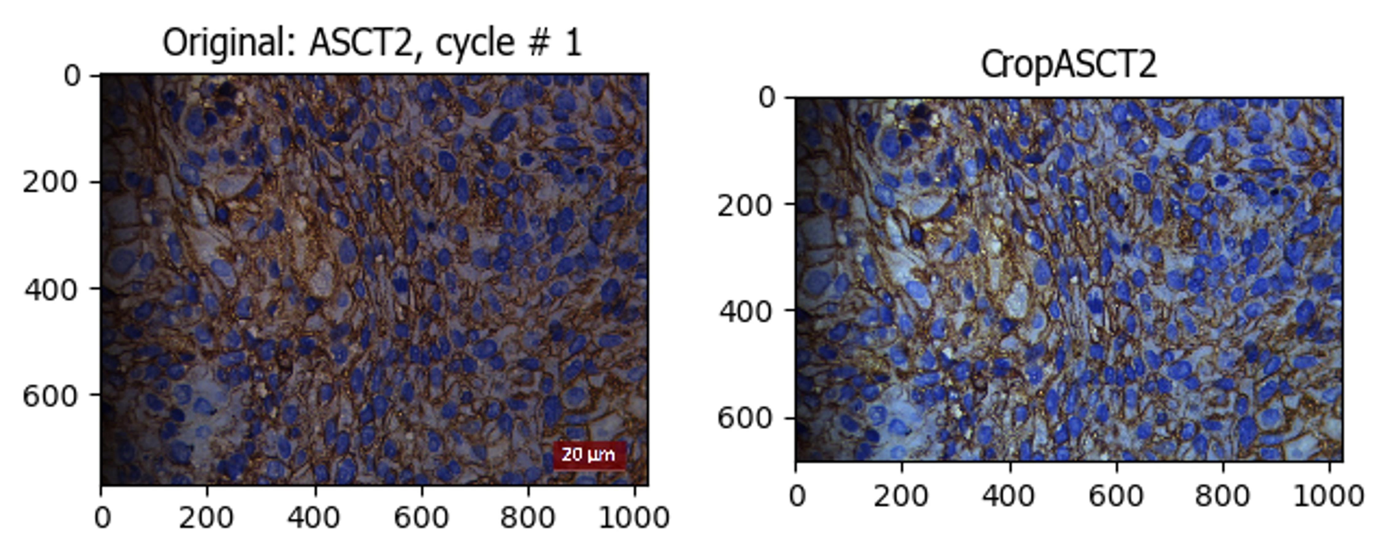
Figure 1. Crop module. Representative screenshots illustrating the cropping of unwanted regions of the image that interfere with image processing.
Note: Use of raw images without embedded scale bars is preferred to avoid introducing non-biological artifacts into the analysis. If scale bars are present, they should be removed using the Crop module prior to downstream processing.
Step 4. ColorToGray module
The ColorToGray module (Figure 2) is used to convert the cropped color IHC image into grayscale representations of individual color components. In brightfield IHC DAB staining, color information (brown DAB and blue hematoxylin) is critical for separating chromogens and improving segmentation. Converting to grayscale channels allows selective processing of specific color information in later modules.
1. Select the input image: “CropProtein” (from the Crop module).
2. Select the conversion method: “Split”. The image is decomposed into separate channels based on the selected color space.
3. Select the image type: “HSV”. The RGB image is converted into hue, saturation, and value (HSV) components. HSV is advantageous for brightfield IHC analysis because hue represents the color type (useful for distinguishing DAB from hematoxylin), saturation reflects the intensity or purity of the color signal, and value represents overall brightness.
4. Convert hue to grayscale: “Yes”. Name the output image: “OrigHue”.
5. Convert saturation to grayscale: “Yes”. Name the output image: “OrigSaturation”.
6. Convert value to grayscale: “Yes”. Name the output image: “OrigValue”.
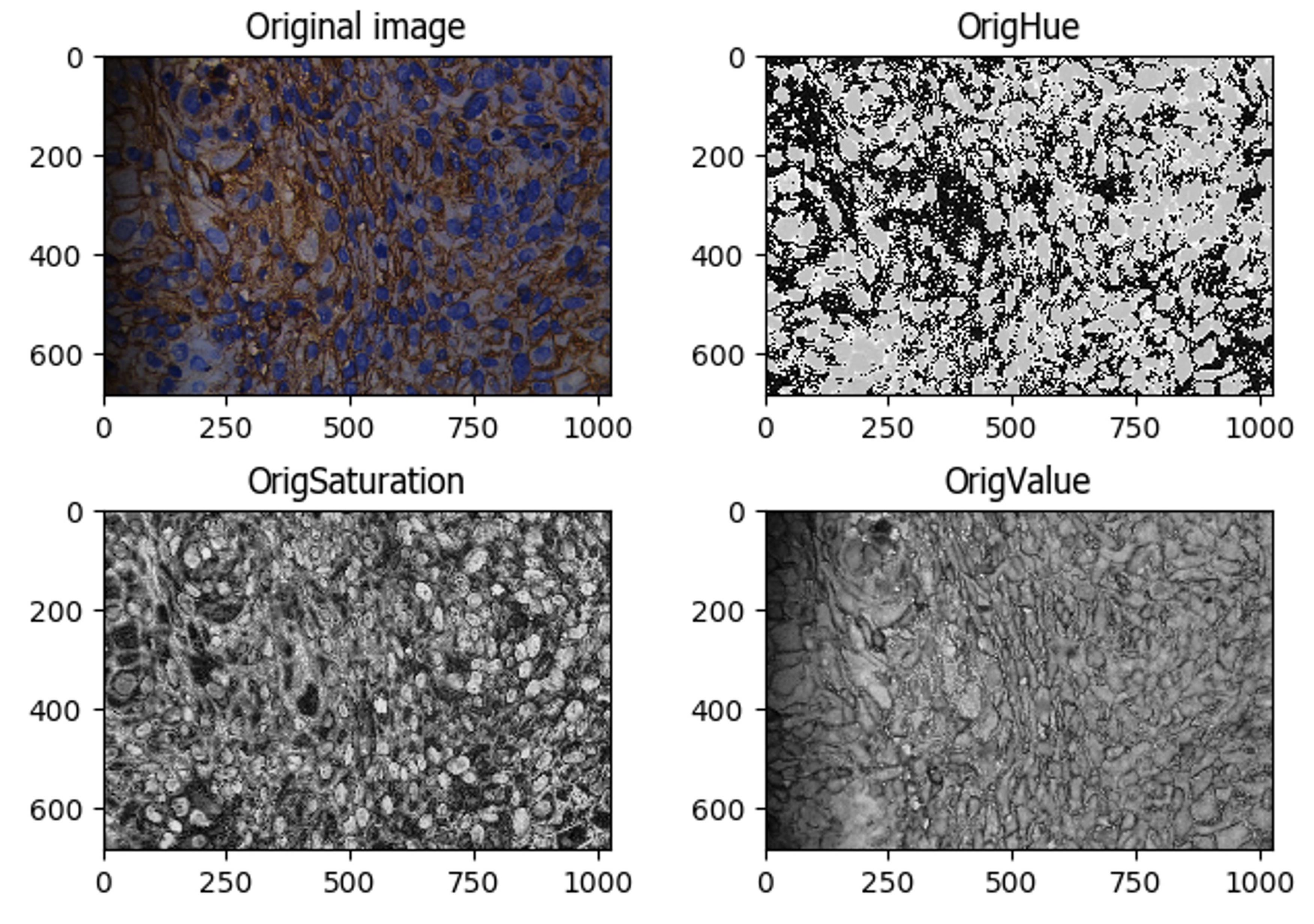
Figure 2. ColorToGray module. Representative screenshot of the module in which the images are converted from RGB to grayscale for the selective processing of color channels.
Step 5. UnmixColors module
The UnmixColors module (Figure 3) separates DAB and hematoxylin chromogens using color deconvolution. It uses color deconvolution to mathematically separate overlapping chromogens within the RGB image. In DAB-based IHC, brown DAB indicates target protein localization (e.g., membrane staining), while blue hematoxylin stains nuclei. Accurate separation is essential for independent segmentation and intensity quantification.
1. Select the input color image: “CropProtein" (from the Crop module).
2. First stain separation: Name the output image: “nuclei_gray”. Stain: “Hematoxylin”.
3. Second stain separation: Name the output image: “protein_gray”. Stain: “DAB”.
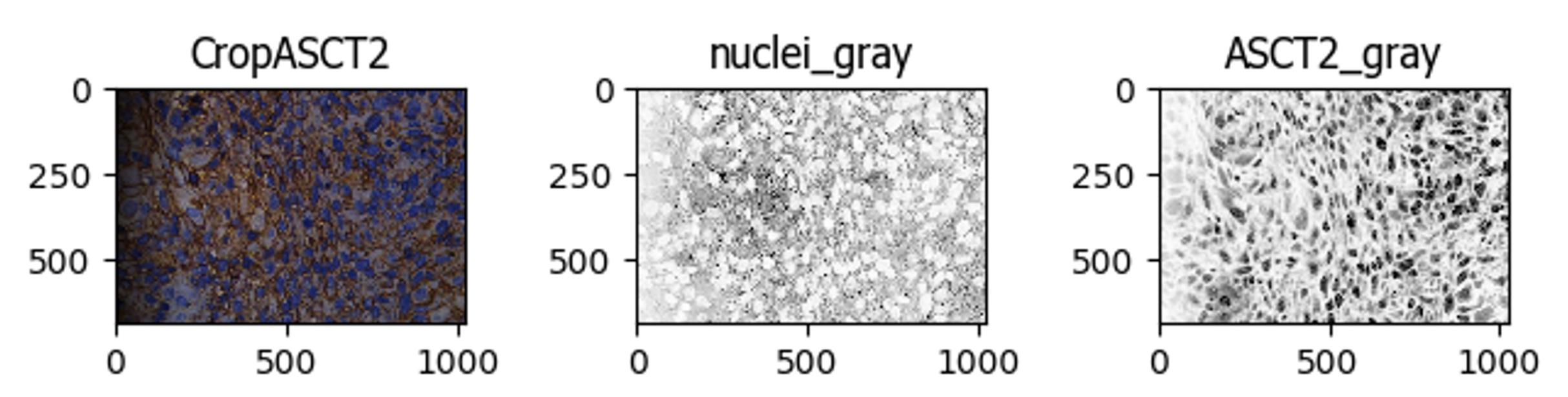
Figure 3. UnmixColors module. Representative outputs of the module showing the separation of DAB and hematoxylin chromogens using color deconvolution.
Step 6. CorrectIlluminationCalculate module
The CorrectIlluminationCalculate module (Figure 4) in CellProfiler is used to estimate background illumination patterns caused by non-uniform lighting conditions in brightfield microscopy. Such variations may arise from microscope optics, lamp intensity fluctuations, or slide thickness. Correcting these artifacts improves segmentation accuracy and ensures reliable intensity measurements.
1. Select the input image: “nuclei_gray” (from the UnmixColors module).
2. Name the output image: “IllumNuclei”.
3. Select how the illumination function is calculated: “Regular”.
4. Dilate objects in the final averaged image: “No”.
5. Rescale the illumination function: “Yes”.
6. Calculate the function for each image individually, or based on all images: “Each”. Illumination correction is computed separately for each image to account for image-to-image variability.
7. Select the smoothing method: “Gaussian Filter”.
8. Select the method to calculate the smoothing filter size: “Manually”.
9. Set smoothing filter size: “80”. A large smoothing filter size (80 pixels) ensures that fine cellular structures are ignored, allowing only large-scale illumination gradients to be modeled.
10. Retain the averaged image: “No”.
11. Retain the dilated image: “No”.
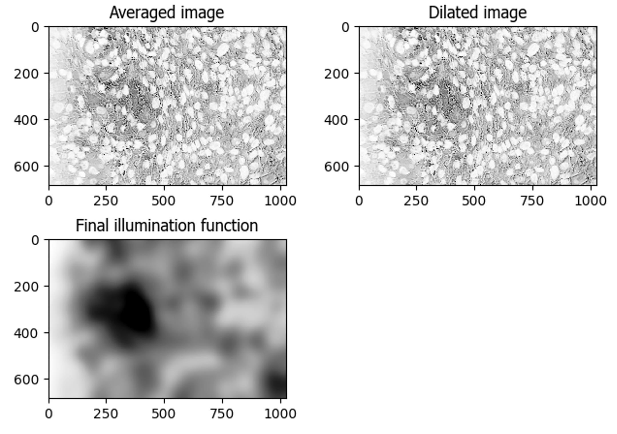
Figure 4. CorrectIlluminationCalculate module. Representative outputs showing correction of background illumination patterns.
Step 7. CorrectIlluminationApply module
The CorrectIlluminationApply module (Figure 5) in CellProfiler is used to apply the previously computed illumination function to the hematoxylin grayscale image. This step corrects uneven background shading and normalizes intensity across the field of view, thereby improving the accuracy and consistency of downstream nuclear segmentation.
1. Select the input image: “nuclei_gray” (from the UnmixColors module).
2. Name the output image: “CorrNuclei”.
3. Select the illumination function: “IllumNuclei” (from the CorrectIlluminationCalculate module).
4. Select how the illumination function is applied: “Divide”. Division is appropriate for correcting multiplicative illumination artifacts commonly observed in brightfield microscopy.
5. Set output image values less than 0 or equal to 0: “Yes”.
6. Set output image values greater than 1 or equal to 1: “Yes”.
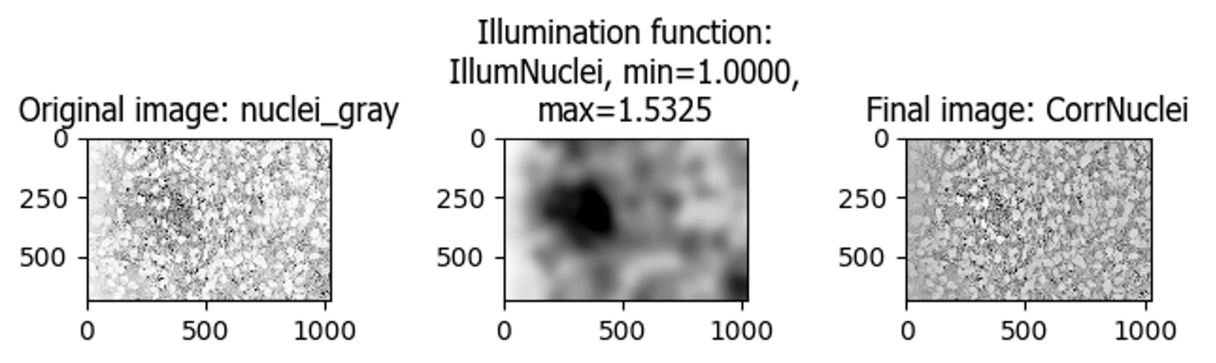
Figure 5. CorrectIlluminationApply module. Representative screenshot showing the application of the previously computed illumination function.
Step 8. IdentifyPrimaryObjects module
The IdentifyPrimaryObjects module (Figure 6) in CellProfiler is used to detect and segment nuclei from the corrected hematoxylin channel (“CorrNuclei”). Accurate nuclear segmentation is critical, as nuclei serve as reference objects for defining whole cells and subsequent membrane regions for DAB intensity quantification.
1. Use advanced settings: “Yes”.
2. Select the input image: “CorrNuclei” (from the CorrectIlluminationApply module).
3. Name the primary objects to be identified: “Nuclei”.
4. Typical diameter of objects (Min, Max): “15–60 pixels”. Objects outside this size range are excluded to remove debris (too small) and merged clusters or artifacts (too large).
5. Discard objects outside the diameter range: “Yes”.
6. Discard objects touching the border of the image: “Yes”.
7. Threshold strategy: “Global”. A single threshold value is applied across the entire image.
8. Thresholding method: “Robust Background”. This method estimates background intensity while excluding outliers, making it suitable for brightfield tissue images.
9. Lower outlier fraction: “0.02”.
10. Upper outlier fraction: “0.6”.
11. Averaging method: “Mean”.
12. Variance method: “Standard deviation”.
13. Number of deviations: “3”.
14. Threshold smoothing scale: “2”.
15. Threshold correction factor: “1”.
16. Lower and upper bounds on threshold: “0.0–1.0”.
17. Method to distinguish clumped objects: “Intensity”.
18. Method to draw dividing lines between clumped objects: “Shape”.
19. Automatically calculate size of smoothing filter for declumping: “Yes”.
20. Automatically calculate minimum allowed distance between local maxima: “Yes”.
21. Speed up by using lower-resolution images to find local maxima: “Yes”.
22. Display accepted local maxima: “No”.
23. Fill holes in identified objects: “After both thresholding and declumping”.
24. Handling of objects if an excessive number is identified: “Continue”.
Note: The selected parameters were optimized for the given image set; however, slight adjustments may be required depending on image resolution, staining intensity, and tissue characteristics.
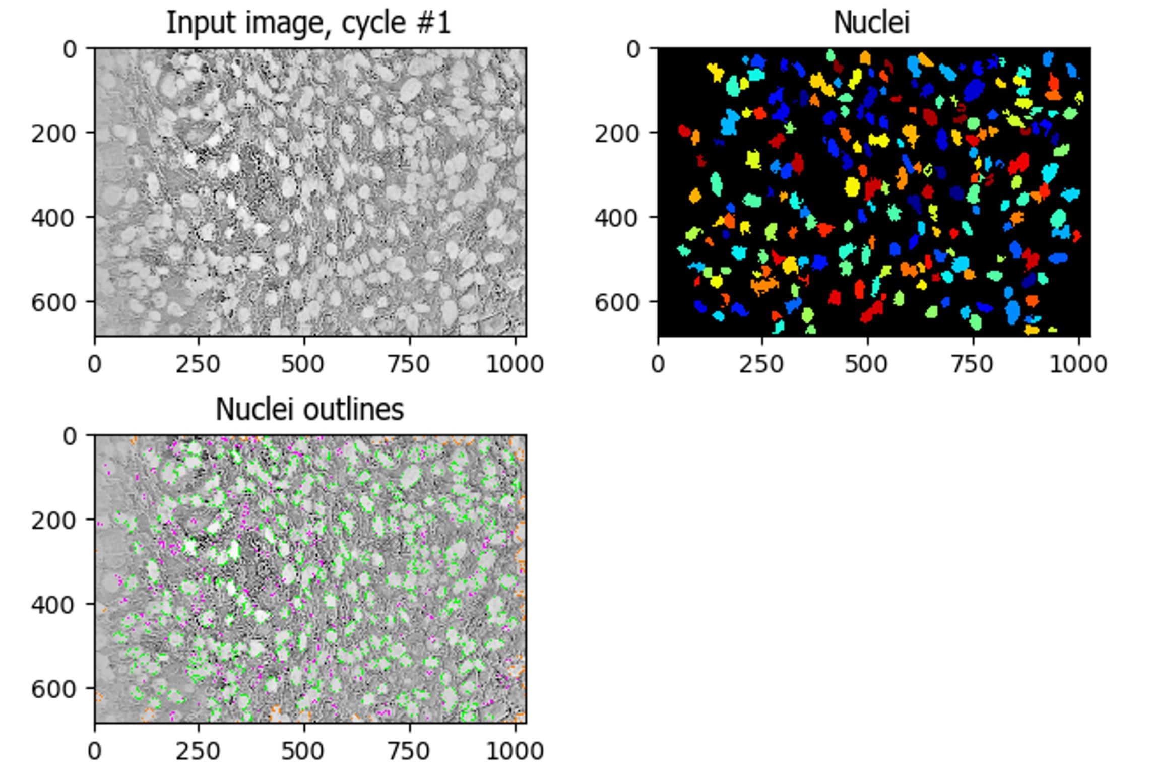
Figure 6. IdentifyPrimaryObjects module. Representative CellProfiler output showing the identification of primary object (nuclei) and segmentation of the nucleus.
Step 9. CorrectIlluminationCalculate module (DAB channel)
The CorrectIlluminationCalculate module (Figure 7) in CellProfiler was applied to the DAB-separated image (“protein_gray”) using the same settings as described in Step 6, with the exception of the smoothing filter size.
1. Input image: “protein_gray”
2. Output image: “IllumProtein”
3. Smoothing filter size: “100” (optimized for DAB channel)
Note: Illumination correction was calculated independently for each microscopic field to compensate for field-specific variations in illumination caused by the microscope optics, light source, and minor differences in tissue thickness. Because the images analyzed were individual brightfield microscopic fields rather than whole-slide images, the predominant intensity variation was technical rather than biological. A large Gaussian smoothing filter (100 pixels) was used to estimate only low-frequency background illumination while preserving local DAB staining patterns.
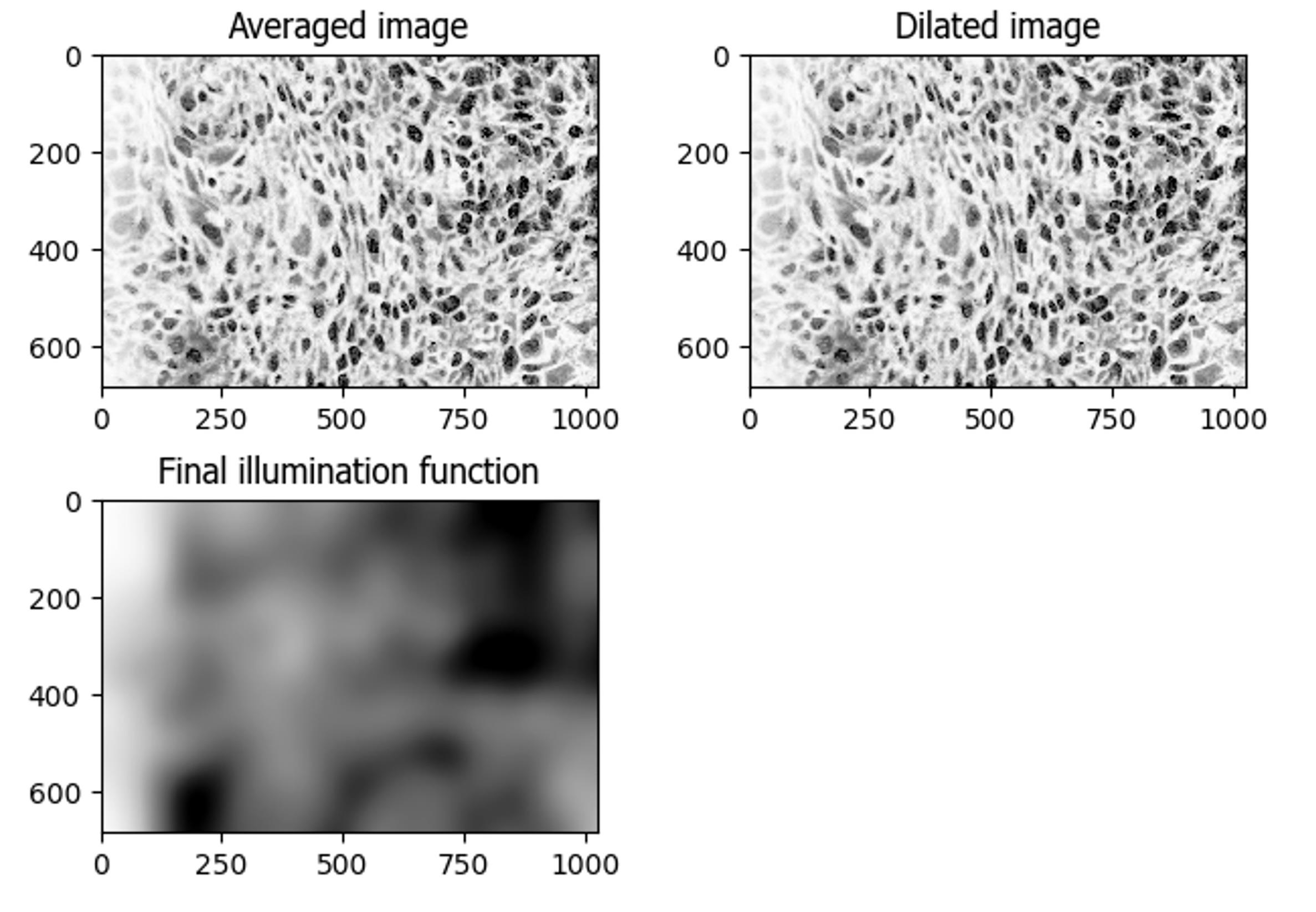
Figure 7. CorrectIlluminationCalculate module. Representative screenshot showing the application of the CorrectIlluminationCalculate Module in DAB-separated images.
Step 10. CorrectIlluminationApply module (DAB channel)
The CorrectIlluminationApply module (Figure 8) in CellProfiler was applied as described in step 7, using:
1. Input image: “protein_gray”
2. Illumination function: “IllumProtein”
3. Output image: “CorrProtein”.
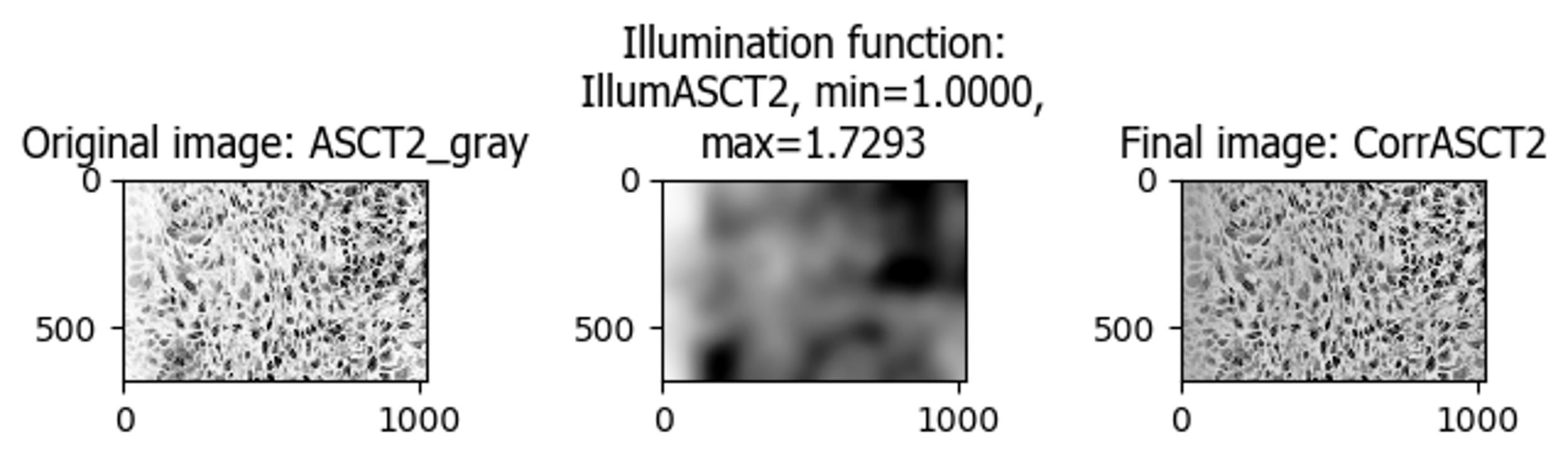
Figure 8. CorrectIlluminationApply module. Representative output showing the application of the module in illumination-corrected DAB-separated images.
Step 11. IdentifySecondaryObjects module
The IdentifySecondaryObjects module (Figure 9) is used to define whole-cell regions using nuclei as seeds for downstream membrane intensity measurement. It expands each segmented nucleus to approximate the full cell boundary. This step is essential because membrane DAB intensity must be measured within defined cellular regions rather than across the entire image.
1. Select the input image: “CorrProtein” (from the CorrectIlluminationApply module).
2. Select the input objects: “Nuclei” (from the IdentifyPrimaryObjects module).
3. Name the objects to be identified: “preCell”.
4. Select the method to identify the secondary objects: “Propagation”. Propagation expands outward from each nucleus based on image intensity gradients and is suitable when DAB staining provides contrast for defining cell boundaries.
5. Threshold strategy: “Global”.
6. Thresholding method: “Minimum Cross-Entropy”. This method determines an optimal threshold by minimizing cross-entropy between foreground and background, making it suitable for DAB images with variable intensity distributions.
7. Threshold smoothing scale: “2”.
8. Threshold correction factor: “1”.
9. Lower and upper bounds on threshold: “0.0–1.0”.
10. Log transform before thresholding: “No”.
11. Regularization factor: “0.05”.
12. Fill holes in identified objects: “Yes”.
13. Discard secondary objects touching the border of the image: “Yes”.
14. Discard the associated primary objects: “No”.
The resulting “preCell” objects represent approximated whole-cell regions derived from nuclear seeds and DAB intensity gradients.
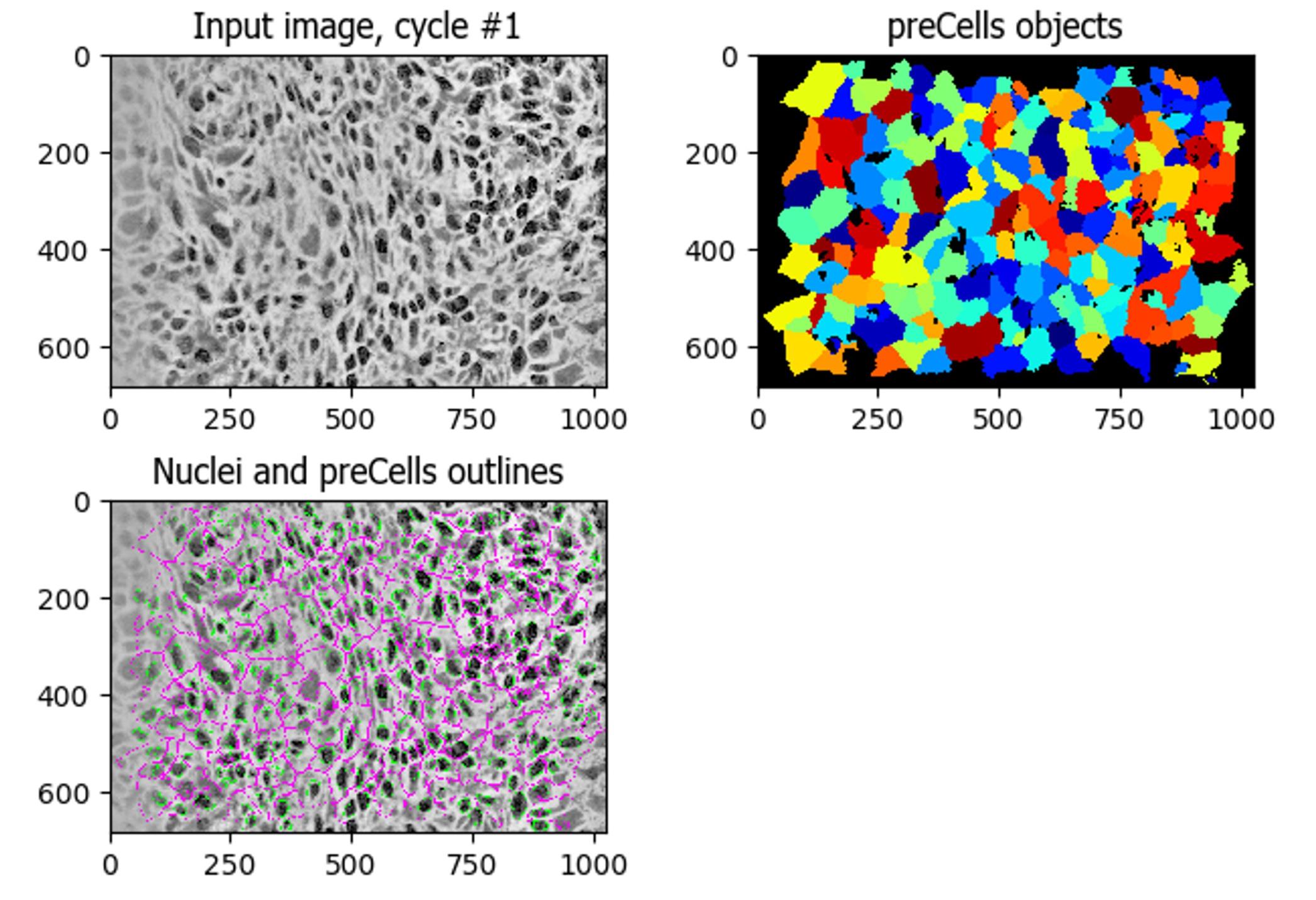
Figure 9. IdentifySecondaryObject module. Representative output showing the expansion of segmented nuclei to generate whole-cell objects using the IdentifySecondaryObjects module. Propagation based on image intensity gradients approximates cell boundaries for subsequent membrane identification.
Step 12. IdentifyTertiaryObjects module
The IdentifyTertiaryObjects module (Figure 10) is used to define membrane-associated regions by excluding nuclear areas from whole-cell objects. It identifies membrane regions by subtracting nuclear objects from the corresponding whole-cell (“preCell”) objects. This enables selective quantification of DAB staining in the non-nuclear compartment.
1. Select the larger identified objects: “preCell” (from the IdentifySecondaryObjects module). These represent the full-cell boundaries.
2. Select the smaller identified objects: “Nuclei” (from the IdentifyPrimaryObjects module). These represent nuclear regions to be excluded.
3. Name the tertiary objects to be identified: “Membrane”.
4. Shrink smaller objects prior to subtraction: “No”.
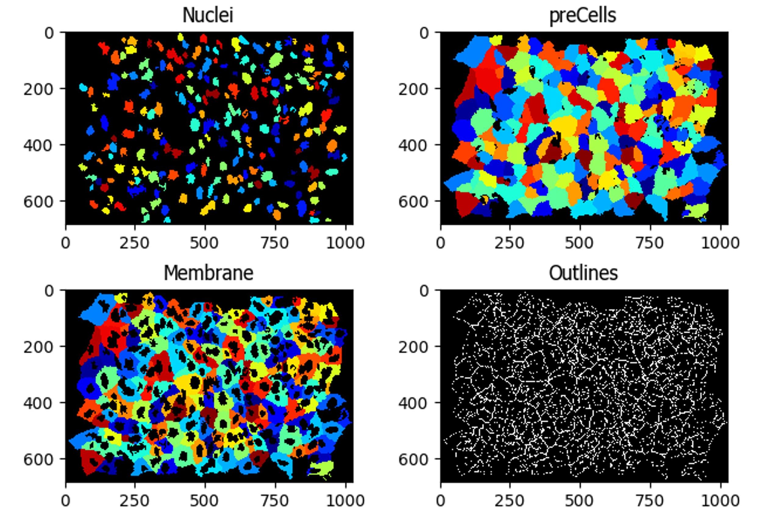
Figure 10. IdentifyTertiaryObjects module. Representative images illustrating the generation of membrane-associated objects by subtracting nuclear regions from whole-cell objects.
Step 13. Threshold module
The Threshold module (Figure 11) is used to convert the grayscale DAB image into a binary image to distinguish positive staining from background. In this step, CellProfiler classifies pixels as either foreground (positive staining) or background based on their intensity values. Since DAB-positive regions appear darker in the unmixed image, thresholding helps isolate the true immunohistochemical signal from weak nonspecific staining and background noise.
1. Select the input image: “Protein_gray” [from the UnmixColors (Step 5) module].
2. Name the output image: “Protein_positive”.
3. Select the threshold strategy: “Global”. The thresholding strategy determines the type of input that is used to calculate the threshold based on the whole image or image sub-regions.
4. Select the thresholding method: “Otsu”. This approach calculates the two classes of pixels (foreground and background) by minimizing the variance within each class.
5. Select whether the thresholding is “Two-class” or “Three-class”. Two-class thresholding distinguishes images based on two classes: foreground (region of interest) and background.
6. Threshold smoothing scale: “0.0”.
7. Threshold correction factor: “1.1”.
8. Lower and upper bounds on threshold: “0.0–1.0”.
9. Log transform before thresholding: “No”.
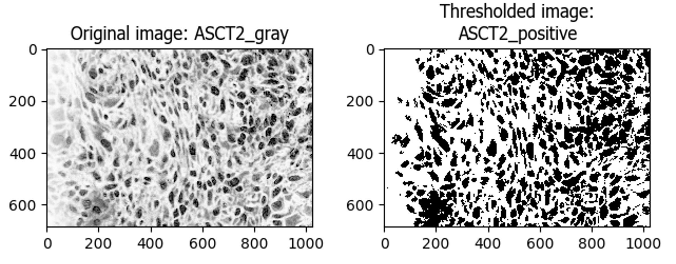
Figure 11. Threshold module. Representative images showing the thresholding of the DAB channel to identify positively stained regions for quantitative analysis.
Step 14. MeasureObjectIntensity module
The MeasureObjectIntensity module (Figure 12) is used to quantify DAB intensity within membrane-associated regions on a per-cell basis. It extracts quantitative intensity features from defined objects. In this workflow, DAB intensity is measured within “Membrane” objects to assess membrane-associated protein expression.
1. Select images to measure: “Protein_gray” (from UnmixColors module).
2. Select objects to measure: “Membrane” (from the IdentifyTertiaryObjects module). Measurement is restricted to membrane-associated regions (whole cell minus nucleus), excluding nuclear signal.
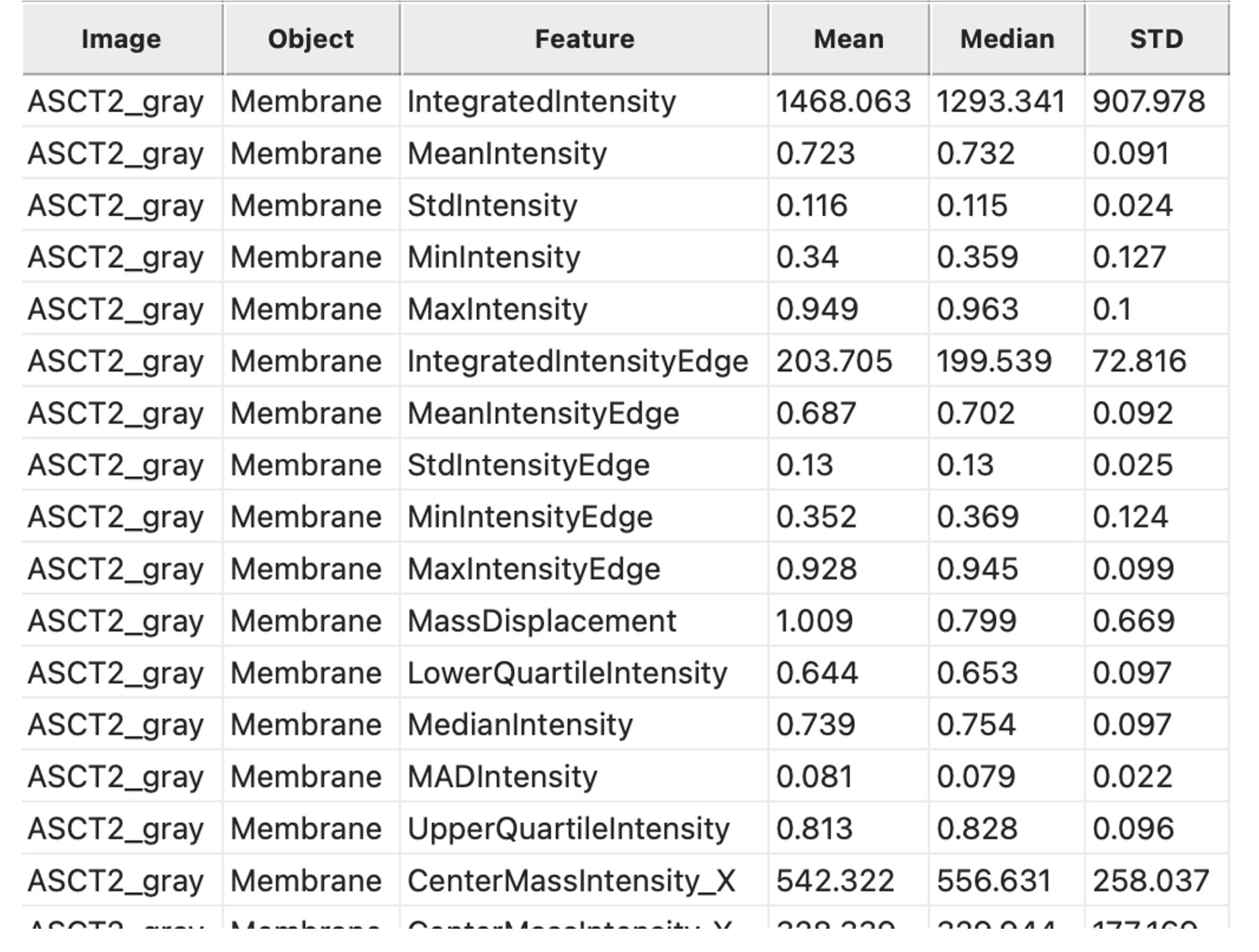
Figure 12. MeasureObjectIntensity module. Representative spreadsheet output generated by the MeasureObjectIntensity module showing membrane-associated DAB intensity measurements and the proportion of positively stained tissue area.
Step 15. MeasureImageAreaOccupied module
The MeasureImageAreaOccupied module (Figure 13) is used to quantify membranous staining within the tissue section and is particularly useful for heterogeneous immunohistochemical patterns where mean intensity alone may not accurately reflect protein expression.
1. Measure the area occupied by: “Binary image”.
2. Select binary images to measure: “Protein_positive” (from the Threshold module).

Figure 13. MeasureImageAreaOccupied module. Representative spreadsheet output generated by the MeasureImageAreaOccupied module showing the proportion of positively stained tissue area.
Note: The image analysis was performed on manually selected microscopic fields containing tumor tissue. The images were cropped to remove the scale bar, thereby containing the tumor region while minimizing background and empty regions. Consequently, the total cropped image area was used as the reference denominator for estimating the proportion of DAB-positive objects. For analyses involving heterogeneous tissue sections or whole-slide images containing variable amounts of stroma or background, the generation of a tissue or tumor region-of-interest mask is recommended to provide a biologically relevant reference area.
Step 16. ExportToSpreadsheet module
The ExportToSpreadsheet module in CellProfiler is used to export all measured object features (e.g., membrane DAB intensity values) into spreadsheet files for further statistical analysis and visualization.
1. Select the column delimiter: “Comma (",")”. Data are exported in CSV format for compatibility with downstream analysis tools.
2. Set the output file location: Default Output Folder.
3. Add a prefix to file names: “Yes”. Filename prefix: [Sample ID].
4. Overwrite existing files without warning: “No”.
5. Add image metadata columns to object data file: “No”.
6. Add image file and folder names to object data file: “No”.
7. Select the measurements to export: “No”.
8. Export per-image summary statistics (mean, median, standard deviation): “No”.
D. Randomization of values
1. Select the required integrated intensity values from the final .csv file obtained from CellProfiler and copy them into a new Microsoft Excel file. Repeat this step for all samples.
2. Since CellProfiler quantifies hundreds to thousands of individual cells per image, random sampling is performed to obtain a representative subset of cells for downstream statistical analysis while avoiding user selection bias.
3. Insert a new column titled “Random Values” adjacent to the obtained intensity values. Use the =RAND() function on Excel and drag and drop to assign random values to all your intensity values (Figure 14).
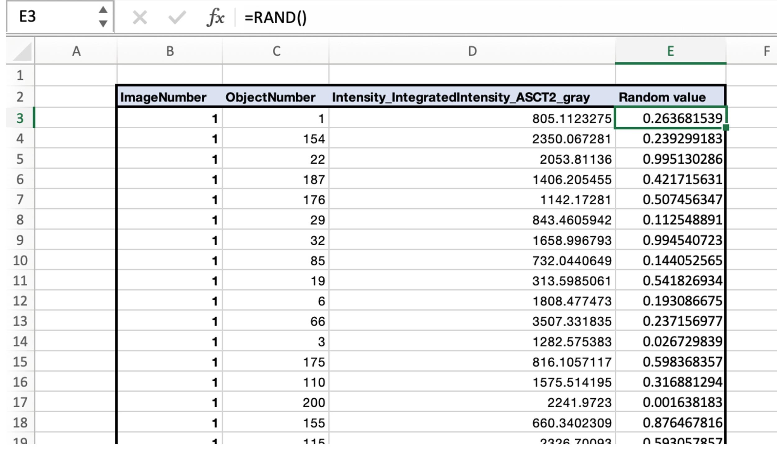
Figure 14. Assignment of random values in Excel. The =RAND() function, which is built into Excel, is used. This assigns a unique number between 0 and 1 to all selected cells. Random values can be assigned to all intensity values by dragging and dropping.
4. Once each sample has been assigned a random value, select the number of cells to be analyzed across all samples so uniformity can be maintained.
5. This Excel file can be visualized graphically through standard statistical packages according to the user’s requirements.
E. Data analysis
1. After random values are assigned, select all data columns, including the column with random numbers.
2. Using the sort function of Excel, sort the Random column (smallest to largest).
3. After sorting, select the first 200 objects or more. The number of objects should be uniform across different sample types.
4. Load a separate Excel page and label the sample name. Copy and paste the 200 objects that were sorted.
5. Repeat for different samples.
6. For visualization and calculation of statistical significance, GraphPad Prism can be used.
Note: The grouped table format was loaded in GraphPad Prism. The Groups were labeled with the sample name, and values were pasted in the column accordingly. The values were analyzed using one-way ANOVA followed by Dunnett’s multiple comparison test. A p-value <0.05 was considered statistically significant. A violin plot was used to visualize the data.
General notes and troubleshooting
General notes
1. Perform all IHC staining under identical experimental conditions using the same antibody dilution, incubation time, chromogen development time, and imaging parameters to minimize technical variability.
2. The CellProfiler parameters described in this protocol were optimized for membrane-associated DAB staining of ASCT2 in FFPE cervical cancer tissues. Minor adjustment of segmentation parameters may be required for other tissue morphologies, biomarkers, and imaging systems.
3. Acquire using identical microscope settings (objective, illumination, exposure time, white balance, and camera settings) for all experimental groups. Avoid modifying brightness, contrast, gamma, or color balance after image acquisition, as these adjustments may affect intensity-based quantification.
4. Capture representative tissue regions while excluding tissue folds, section edges, necrotic areas, staining artifacts, air bubbles, and out-of-focus fields.
5. Use high-quality brightfield images with adequate resolution and minimal background staining. Images should be acquired under consistent illumination to ensure accurate color deconvolution and segmentation.
6. If images contain embedded scale bars, remove them using the Crop module before analysis to prevent non-biological objects from being detected during segmentation.
7. Analyze all samples using the same CellProfiler pipeline and parameter settings throughout the study to ensure reproducibility and comparability between experimental groups.
8. This protocol deals with a small cohort of manually acquired images. However, larger datasets can be processed with available metadata and sample IDs derived from high-throughput imaging systems using CellProfiler.
Troubleshooting
| Problem | Possible cause | Solution |
|---|---|---|
| Poor nuclear segmentation | Weak hematoxylin staining or uneven illumination | Increase hematoxylin staining quality and verify illumination correction settings before segmentation |
| Membrane boundaries are not accurately detected | Weak membrane DAB staining or incorrect propagation parameters | Adjust the threshold correction factor or propagation settings in the IdentifySecondaryObjects module and verify staining quality |
| Excessive background detected as positive staining | High nonspecific DAB staining or tissue artifacts | Reduce DAB development time, optimize antibody dilution, and exclude artifact-containing regions before analysis |
| Cells are merged into large objects | Incorrect object diameter or threshold parameters | Modify the minimum and maximum object diameter and optimize declumping settings in the IdentifyPrimaryObjects module |
| Large variation between images | Different microscope illumination or camera settings | Acquire all images using identical microscope, camera, and exposure settings throughout the experiment |
| Scale bar or labels detected as objects | Images contain embedded annotations | Remove the scale bar and annotations using the Crop module before analysis |
| Low reproducibility between datasets | Different CellProfiler parameters used for different image sets | Use a single validated pipeline with identical parameter settings for all images in the study |
| CellProfiler processing is slow | Large image size or insufficient computer memory | Close unnecessary applications, analyze images in batches, or reduce image size while preserving sufficient resolution for segmentation |
Validation of protocol
The CellProfiler workflow was validated using ASCT2 immunohistochemical staining in FFPE human cervical cancer tissue sections representing high, low, and negative ASCT2 expression (Figure S1). Representative brightfield images demonstrated distinct membrane-associated DAB staining intensities among the groups (Figure 15A). CellProfiler segmentation consistently identified the membrane-associated, non-nuclear cellular compartment across staining intensities (Figure 15B). DAB-positive pixels were subsequently identified using intensity thresholds, and integrated DAB intensity within the segmented compartment was quantified (Figure 15C). ASCT2-high tissues showed significantly greater integrated DAB intensity than ASCT2-low and negative controls (Figure 15D). Manual H-score analysis performed with pathologist assistance similarly showed significantly higher scores in ASCT2-high tissues compared with the other groups (Figure 15E). Statistical significance was assessed using one-way ANOVA followed by Dunnett’s multiple-comparison test. Overall, the CellProfiler workflow (File S1, Video S1) reliably distinguished ASCT2 expression levels and generated quantitative measurements consistent with conventional H-score assessment, supporting its utility for membrane-associated DAB IHC quantification.
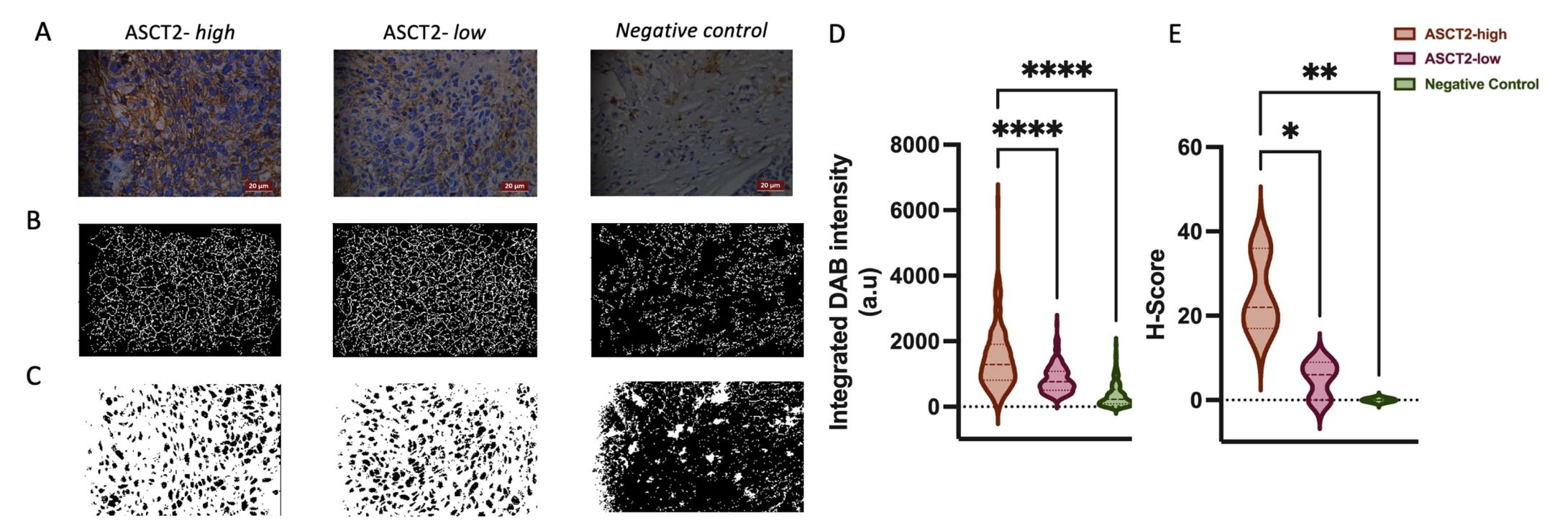
Figure 15. Validation of the CellProfiler workflow for quantification of ASCT2 DAB immunohistochemistry in FFPE human cervical cancer tissue sections. (A ) Representative brightfield images of DAB-immunostained FFPE human cervical cancer tissue sections demonstrating ASCT2-high, ASCT2-low, and negative control staining. Images were acquired at 40× magnification. Scale bars, 20 μm. (B) Representative segmentation outputs generated by CellProfiler showing the segmented membrane-associated (non-nuclear) cellular compartment used for quantitative analysis. Nuclei were first identified from the hematoxylin channel, and the non-nuclear cellular compartment was generated by propagation from the nuclei using the corrected DAB image. (C) Representative thresholded images used for quantification of DAB-positive regions in the respective groups. White pixels represent DAB-positive signals, and black pixels represent DAB-negative signals. (D) Quantification of integrated DAB intensity (IntegratedIntensity, arbitrary intensity units [a.u.]) measured within the segmented membrane-associated (non-nuclear) cellular compartment using the CellProfiler MeasureObjectIntensity module. Higher values indicate greater total membrane-associated ASCT2 immunoreactivity. Data were obtained from n = 3 independent FFPE cervical cancer specimens each, for ASCT2-high, ASCT2-low, and negative control (no primary antibody), analyzing four fields per specimen with 200 randomly selected cells per group. Statistical significance was determined using one-way ANOVA followed by Dunnett’s multiple-comparison test. ****P < 0.0001. (E) Manual H-score analysis of ASCT2 immunohistochemical staining in FFPE human cervical cancer tissue sections. H-scores were determined by a pathologist using the conventional semi-quantitative scoring method based on staining intensity and the percentage of positively stained tumor cells. Higher H-scores indicate stronger ASCT2 membrane-associated immunoreactivity. The H-score results demonstrate a staining pattern consistent with the CellProfiler-derived integrated DAB intensity (a.u.), supporting the validity of the automated quantification. Data represent n = 3 independent tissue specimens. Statistical significance was determined using one-way ANOVA followed by Dunnett’s multiple-comparison test. *P < 0.05, **P < 0.01.
Supplementary information
The following supporting information can be downloaded here:
1. File S1. CellProfiler pipeline
2. Figure S1. Representative images for ASCT2-high, ASCT2-low, and negative control
3. Video S1. Tutorial video of the CellProfiler workflow
Acknowledgments
We thank the Department of Pathology, Sri Ramachandra Institute of Higher Education and Research, for the processing of tissues and preparation of slides.
Part of this work was funded by Board of Research in Nuclear Sciences (BRNS) No. 44/14/10/2025-BRNS/1288 to Rajesh Kumar Gandhirajan.
Author contributions
Conceptualization, R.K.G.; Investigation, K.K., N.R., N.N., R.M.; Writing—Original Draft, K.K., N.R., N.N., R.M.; Writing—Review & Editing, R.M., R.K.G., G.V., L.D.J.; Funding acquisition, R.K.G.; Supervision, R.K.G., G.V., L.D.J.
Competing interests
The authors declare no conflicts of interest.
Ethical considerations
Ethics approval (REF: IEC-NI/22/JUL/83/94) was obtained from the Institutional Ethics Committee of Sri Ramachandra Institute of Higher Education and Research.
References
- Ramos-Vara, J. A. (2005). Technical Aspects of Immunohistochemistry. Vet Pathol. 42(4): 405–426. https://doi.org/10.1354/vp.42-4-405
- Kim, S. W., Roh, J. and Park, C. S. (2016). Immunohistochemistry for Pathologists: Protocols, Pitfalls, and Tips. J Pathol Transl Med. 50(6): 411–418. https://doi.org/10.4132/jptm.2016.08.08
- Shi, S. R., Liu, C. and Taylor, C. R. (2007). Standardization of Immunohistochemistry for Formalin-fixed, Paraffin-embedded Tissue Sections Based on the Antigen-retrieval Technique: From Experiments to Hypothesis. J Histochem Cytochem. 55(2): 105–109. https://doi.org/10.1369/jhc.6p7080.2006
- Goldsmith, J. D., Troxell, M. L., Roy-Chowdhuri, S., Colasacco, C. F., Edgerton, M. E., Fitzgibbons, P. L., Fulton, R., Haas, T., Kandalaft, P. L., Kalicanin, T., et al. (2024). Principles of Analytic Validation of Immunohistochemical Assays: Guideline Update. Arch Pathol Lab Med. 148(6): e111–e153. https://doi.org/10.5858/arpa.2023-0483-cp
- Taylor, C. R. and Levenson, R. M. (2006). Quantification of immunohistochemistry—issues concerning methods, utility and semiquantitative assessment II. Histopathology. 49(4): 411–424. https://doi.org/10.1111/j.1365-2559.2006.02513.x
- Rizzardi, A. E., Johnson, A. T., Vogel, R. I., Pambuccian, S. E., Henriksen, J., Skubitz, A. P., Metzger, G. J. and Schmechel, S. C. (2012). Quantitative comparison of immunohistochemical staining measured by digital image analysis versus pathologist visual scoring. Diagn Pathol. 7(1): 42. https://doi.org/10.1186/1746-1596-7-42
- Madabhushi, A. and Lee, G. (2016). Image analysis and machine learning in digital pathology: Challenges and opportunities. Med Image Anal. 33: 170–175. https://doi.org/10.1016/j.media.2016.06.037
- Gurcan, M., Boucheron, L., Can, A., Madabhushi, A., Rajpoot, N. and Yener, B. (2009). Histopathological Image Analysis: A Review. IEEE Rev Biomed Eng. 2: 147–171. https://doi.org/10.1109/rbme.2009.2034865
- Carpenter, A. E., Jones, T. R., Lamprecht, M. R., Clarke, C., Kang, I. H., Friman, O., Guertin, D. A., Chang, J. H., Lindquist, R. A., Moffat, J., et al. (2006). CellProfiler: image analysis software for identifying and quantifying cell phenotypes. Genome Biol. 7(10): R100. https://doi.org/10.1186/gb-2006-7-10-r100
- McQuin, C., Goodman, A., Chernyshev, V., Kamentsky, L., Cimini, B. A., Karhohs, K. W., Doan, M., Ding, L., Rafelski, S. M., Thirstrup, D., et al. (2018). CellProfiler 3.0: Next-generation image processing for biology. PLoS Biol. 16(7): e2005970. https://doi.org/10.1371/journal.pbio.2005970
- Van Eycke, Y. R., Allard, J., Salmon, I., Debeir, O. and Decaestecker, C. (2017). Image processing in digital pathology: an opportunity to solve inter-batch variability of immunohistochemical staining. Sci Rep. 7(1): e1038/srep42964. https://doi.org/10.1038/srep42964
- Roszkowiak, L., Korzynska, A., Siemion, K., Zak, J., Pijanowska, D., Bosch, R., Lejeune, M. and Lopez, C. (2021). System for quantitative evaluation of DAB&H-stained breast cancer biopsy digital images (CHISEL). Sci Rep. 11(1): 9291. https://doi.org/10.1038/s41598-021-88611-y
- Deng, Y., Cai, B. and Wang, X. (2025). A fully automated quantitative analysis method based on deep learning algorithms for immunohistochemical staining expression intensities. Intelligent Oncology 1(3): 256–264. https://doi.org/10.1016/j.intonc.2025.06.001
- Ruifrok, A. C., Katz, R. L. and Johnston, D. A. (2003). Comparison of Quantification of Histochemical Staining By Hue-Saturation-Intensity (HSI) Transformation and Color-Deconvolution. Anal Quant Cytol Histol. 11(1): 85–91. https://doi.org/10.1097/00129039-200303000-00014
Article Information
Publication history
Received: Jun 2, 2026
Accepted: Aug 4, 2026
Available online: Aug 25, 2026
Published: Sep 20, 2026
Copyright
© 2026 The Author(s); This is an open access article under the CC BY-NC license (https://creativecommons.org/licenses/by-nc/4.0/).
How to cite
Krishnakumar, K., Rasheed, N., Nithyanandan, N., Murali, R., Joseph, L. D., Venkatraman, G. and Gandhirajan, R. K. (2026). Digital Quantification of Membrane DAB Immunohistochemical Staining in FFPE Cervical Cancer Tissues Using an Open-Source CellProfiler Pipeline. Bio-protocol 16(18): e5817. DOI: 10.21769/BioProtoc.5817.

 Download Citation in RIS Format
Category
Bioinformatics and Computational Biology
Cell Biology > Cell imaging > Fixed-cell imaging
Cancer Biology > General technique > Biochemical assays
Do you have any questions about this protocol?
Post your question to gather feedback from the community. We will also invite the authors of this article to respond.
 Post a Question


