


- Protocols

- Articles and Issues
- For Authors
- About
- Become a Reviewer


A MATLAB-Based Image Processing Protocol for Quantitative Differentiation of Diseased and Healthy Plant Tissue From Digital Leaf Images



(*Contributed equally to this work, §Technical contact: pankajborahmajuli@gmail.com) Published: Vol 16, Iss 16, Aug 20, 2026 DOI: 10.21769/BioProtoc.5798 Views: 257
Reviewed by: Ying LiAnonymous reviewer(s)
 PDF
PDF  Ask a question
Original research article
The authors used this protocol in:

Mar 2026
Advertisement


Protocol Collections
Comprehensive collections of detailed, peer-reviewed protocols focusing on specific topics




Abstract
Accurate quantification of plant disease severity is essential for evaluating host–pathogen interactions and assessing the effectiveness of disease management strategies. Traditional visual scoring methods and manual estimation of infected tissue are widely used but are often subjective and prone to observer bias. Digital image analysis offers an objective alternative by enabling automated identification and quantification of symptomatic plant tissues based on color and spatial characteristics.
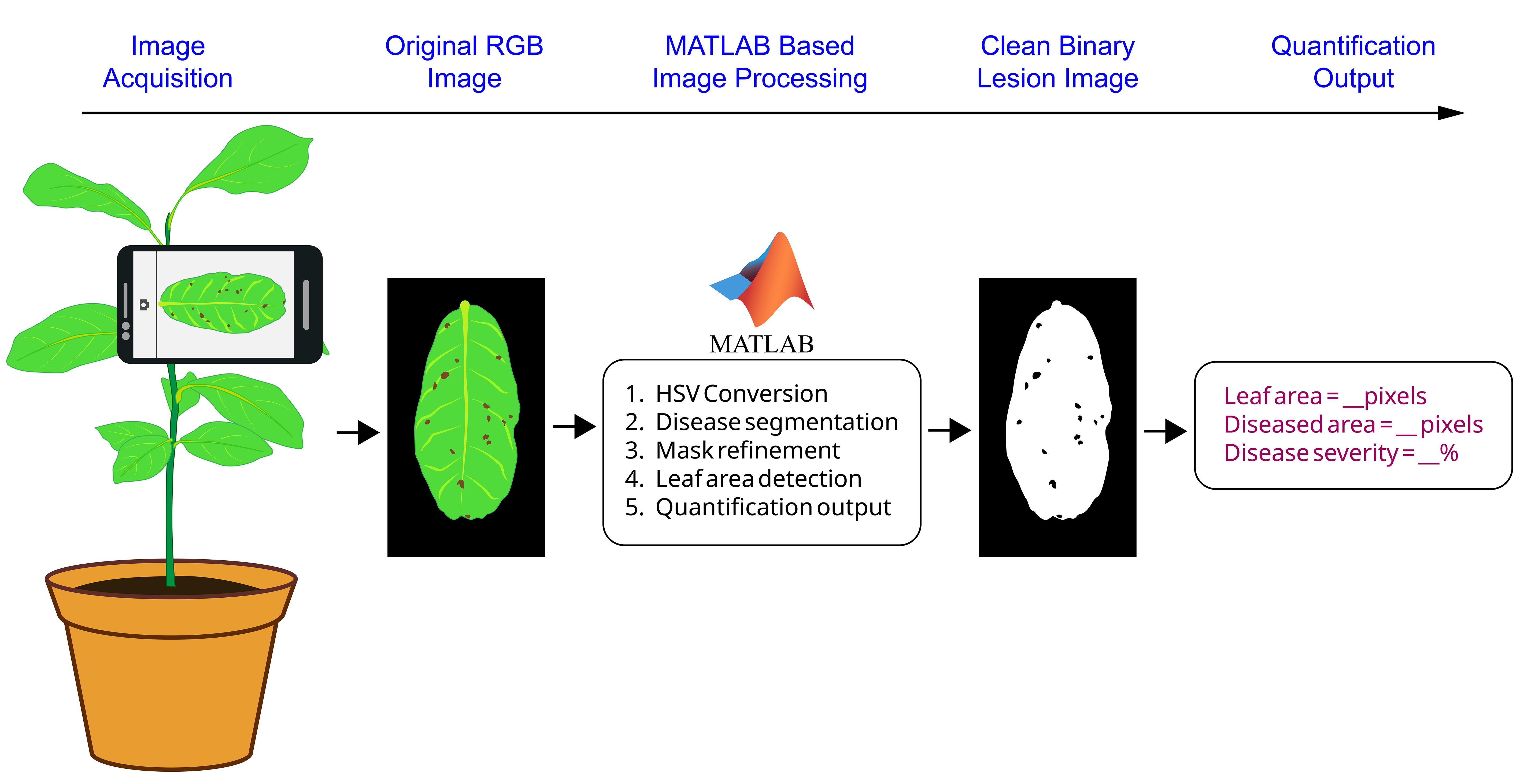
Here, we present a MATLAB-based image processing protocol for differentiating diseased and healthy plant tissue from digital leaf images. The workflow involves acquisition of standardized leaf images, conversion of RGB images into hue-saturation-value (HSV) color space, segmentation of diseased tissue using defined HSV thresholds, refinement of the segmented mask through morphological operations, and extraction of the whole leaf area. The protocol then calculates the diseased area and total leaf area in pixels and computes the percentage of infected tissue. The method uses MATLAB together with the Image Processing Toolbox and can be implemented using simple scripts. This protocol enables rapid and reproducible quantification of disease severity in plant leaves exhibiting visually distinct symptoms such as necrotic lesions or blight patches. By minimizing observer bias and providing quantitative measurements of infected area, the protocol offers a practical and reproducible approach for plant disease phenotyping and evaluation of disease management strategies across diverse plant-pathogen systems where diseased tissues can be clearly distinguished from healthy tissues under reasonably controlled imaging conditions.
Key features
• A reproducible MATLAB-based workflow for separating diseased and healthy plant tissue using color-space segmentation.
• Applicable to plant diseases where symptomatic tissue contrasts clearly with healthy tissue (necrosis, blight lesions, rot patches).
• Requires digital leaf images, MATLAB, and the MATLAB Image Processing Toolbox for image processing and disease quantification.
• Enables rapid calculation of diseased leaf area and disease severity using automated pixel-based quantification.
Keywords: Plant disease phenotyping Image-based disease quantification
MATLAB image processing
Leaf lesion segmentation
Disease severity analysis
Digital plant pathology
Image-based disease quantification
MATLAB image processing
Leaf lesion segmentation
Disease severity analysis
Digital plant pathology
Graphical overview
Background
Accurate quantification of plant disease severity is fundamental for studying plant–pathogen interactions, evaluating disease management strategies, and screening host resistance. Traditionally, disease severity has been assessed using visual rating scales or by estimating the percentage of symptomatic tissue on plant organs. Although such approaches are widely used in plant pathology, they are inherently subjective and may introduce observer bias and variability among evaluators [1,2]. These limitations can reduce reproducibility and may affect the statistical interpretation of disease assessment in experimental studies.
To overcome these constraints, digital image analysis has increasingly been adopted as a more objective and reproducible approach for plant disease phenotyping. Image-based disease assessment enables automated detection and quantification of symptomatic regions by analyzing color, texture, and spatial characteristics of infected tissues. Several studies have demonstrated that image analysis methods can significantly improve accuracy and consistency in disease measurement compared to visual estimates [3,4]. Such approaches are particularly effective for diseases that produce visible symptoms such as necrotic lesions, blights, spots, or rotting tissues that contrast clearly with healthy plant tissue.
Among the different approaches used in image-based disease detection, color-space segmentation has proven to be particularly effective for separating symptomatic and healthy regions in plant images. The hue-saturation-value (HSV) color space is commonly used in plant image analysis because it separates chromatic information from intensity, making it more robust to variations in illumination compared to the traditional RGB color model [5]. HSV-based segmentation has been successfully applied in several plant phenotyping studies, including leaf segmentation, stress detection, and disease symptom quantification.
Image analysis pipelines often combine color segmentation with morphological operations to improve the accuracy of tissue classification. Morphological image processing techniques such as opening, closing, and hole filling are widely used to remove noise, refine segmented regions, and generate continuous masks representing diseased areas [6]. When combined with pixel-based area calculation, these techniques allow precise measurement of diseased tissue relative to total leaf area, enabling quantitative estimation of disease severity.
Various image analysis platforms, such as ImageJ, specialized plant phenotyping software, and machine learning–based tools have been developed for plant disease quantification [4,7]. However, many of these systems require specialized plugins, large training datasets, or complex workflows that may limit their accessibility for routine experimental use. In contrast, simple threshold-based segmentation approaches implemented in scripting environments such as MATLAB provide a flexible and reproducible alternative for disease quantification when symptoms exhibit clear visual contrast with healthy tissue and images are acquired under reasonably controlled conditions. The present protocol does not introduce a new image-processing algorithm; rather, it provides a detailed, step-by-step implementation of an established HSV threshold-based workflow that can be readily adopted, reproduced, and adapted by researchers for routine disease quantification.
The protocol described here provides a MATLAB-based workflow for quantitative differentiation of diseased and healthy plant tissue from digital leaf images using HSV color segmentation combined with morphological image processing. The method involves the acquisition of standardized leaf images, the conversion of RGB images to HSV color space, the segmentation of diseased regions based on defined threshold ranges, the refinement of the segmented mask using morphological operations, and pixel-based quantification of diseased and total leaf area. The protocol requires MATLAB together with the Image Processing Toolbox and does not depend on machine learning models or external image-analysis software.
Although the method was developed using citrus canker symptoms, the workflow may be adapted to other plant diseases that produce visually distinguishable symptoms, such as necrotic lesions, blights, leaf spots, anthracnose, or other forms of conspicuous tissue discoloration. Because segmentation relies on fixed HSV threshold values, users may need to recalibrate the threshold ranges and associated image-processing parameters when applying the protocol to different plant species, disease symptoms, imaging systems, or illumination conditions. Accordingly, this protocol is intended primarily as a practical, reproducible workflow for disease quantification under reasonably controlled imaging conditions rather than as a universally applicable segmentation method.
Materials and reagents
Biological materials
Plant leaves showing visually distinguishable disease symptoms, photographed in situ while attached to the plant (Citrus limon, cultivar Kaji Nemu) (plants maintained at the Experimental Farm, Department of Horticulture, Assam Agricultural University, Jorhat, Assam, India; plants used in greenhouse experiments for citrus canker caused by Xanthomonas citri pv. citri).
Laboratory supplies
1. Field notebook for labeling and tracking photographed samples
2. Plant labels or sample identification tags
3. Measuring scale
Equipment
1. Smartphone camera capable of capturing high-resolution RGB images (Apple Inc., model: iPhone 16)
2. Computer or laptop capable of running MATLAB. Recommended minimum specifications: processor, Intel i3 or equivalent; RAM ≥ 4 GB; operating system, Windows/Linux/macOS
3. Tripod stabilizer for the smartphone camera (optional but recommended for consistent image capture) (IMS Mercantiles Pvt. Ltd., catalog number: DTR 550 LW)
Software and datasets
1. MATLAB R2014b (MathWorks, Natick, MA, USA)
2. MATLAB Image Processing Toolbox (required for execution of the workflow)
3. MATLAB script for segmentation of diseased and healthy leaf tissue and pixel-based area calculation (included in this protocol)
4. Digital images in JPEG (.jpg, .jpeg) or PNG (.png) format acquired under reasonably uniform illumination and against a contrasting background
5. GitHub repository containing the MATLAB source code, README file with installation and execution instructions, and representative example image(s): https://github.com/pankajborahmajuli-source/Leaf-Disease-Detection-MATLAB-Code/blob/main/README.md
6. Representative leaf images used for validation of the protocol are available in the associated research article [8] where the method was applied
7. (Optional) GNU Octave (with the Image package installed) may also be used after minor syntax modifications, including replacement of MATLAB-specific functions where necessary
Software compatibility
This workflow was developed and tested using MATLAB R2014b together with the Image Processing Toolbox. The function im2bw is retained to ensure compatibility with MATLAB R2014b. In newer MATLAB releases, imbinarize may be used as the recommended alternative with only minor syntax modifications. The workflow may also be adapted for GNU Octave after installation of the Image package and minor adjustments to MATLAB-specific syntax.
Procedure
A. Image acquisition of symptomatic leaves
1. Select plants showing visible disease symptoms on leaves. Choose leaves where diseased tissue, such as necrotic lesions or brown lesions, contrasts clearly with healthy green tissue.
2. Ensure that the selected leaf surface is clearly visible and not overlapped by neighboring leaves or plant structures.
3. Capture the image while the leaf remains attached to the plant using the smartphone camera listed in the Equipment section.
4. Position the camera 25–30 cm from the leaf surface and hold the camera perpendicular to the leaf plane to minimize geometric distortion.
5. Capture the image under uniform natural or diffused lighting conditions. Avoid direct sunlight, strong shadows, or reflective glare on the leaf surface.
6. Ensure that the entire leaf area is visible within the image frame and that symptomatic regions are clearly distinguishable from healthy tissue.
7. Capture images using the native resolution of the smartphone camera (minimum recommended resolution: 8 megapixels).
8. Save the image in JPEG or PNG format and transfer the image file to the computer used for MATLAB analysis. Representative symptomatic leaves photographed in situ prior to image processing are shown in Figure 1.
Critical: Maintain consistent camera distance, orientation, and illumination conditions for all images collected within the same experiment to ensure reliable color-based segmentation. For optimal performance, images should be captured under reasonably uniform illumination using consistent camera settings and against a plain, contrasting background. Strong shadows, reflective glare, complex backgrounds, overlapping leaves, or substantial variation in illumination may reduce segmentation accuracy and may require recalibration of the HSV threshold values before analysis.
Note: The workflow accepts RGB leaf images in JPEG (.jpg, .jpeg) and PNG (.png) formats. Images should preferably contain a single clearly visible leaf with visually distinguishable disease symptoms. Images that do not satisfy these criteria may produce inaccurate segmentation results and should be reacquired whenever possible.
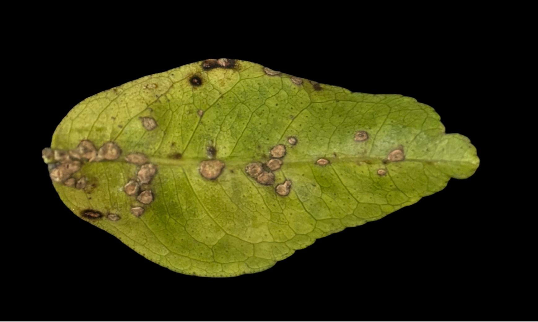
Figure 1. Representative progression of citrus canker symptoms on a lemon leaf at 60 days after inoculation with Xanthomonas citri. Image published with permission from the journal Vegetos, Springer Nature, eISSN: 2229-4473.
B. Importing images into MATLAB
1. Transfer the captured image files to the computer running MATLAB R2014b.
2. Place all images to be analyzed in a single working directory.
3. Open MATLAB and set the working directory to the folder containing the images.
4. Execute the MATLAB script described in this protocol to initiate the image processing workflow. The complete MATLAB code used for the analysis is provided at the end of the Procedure section.
5. When the file selection dialog appears, select the image to be analyzed.
6. MATLAB loads the selected image and displays the original leaf image (Figure 2).
Expected outcome: After selecting the image file, MATLAB imports the RGB image and displays it in a figure window (Figure 2). The imported image serves as the input for all subsequent processing steps, including HSV conversion, disease segmentation, morphological refinement, and disease-area calculation. Users should visually confirm that the selected image has been imported correctly and that the entire leaf is clearly visible before proceeding.
Pause point: Image files can be stored after acquisition and analyzed later without affecting the analysis workflow.
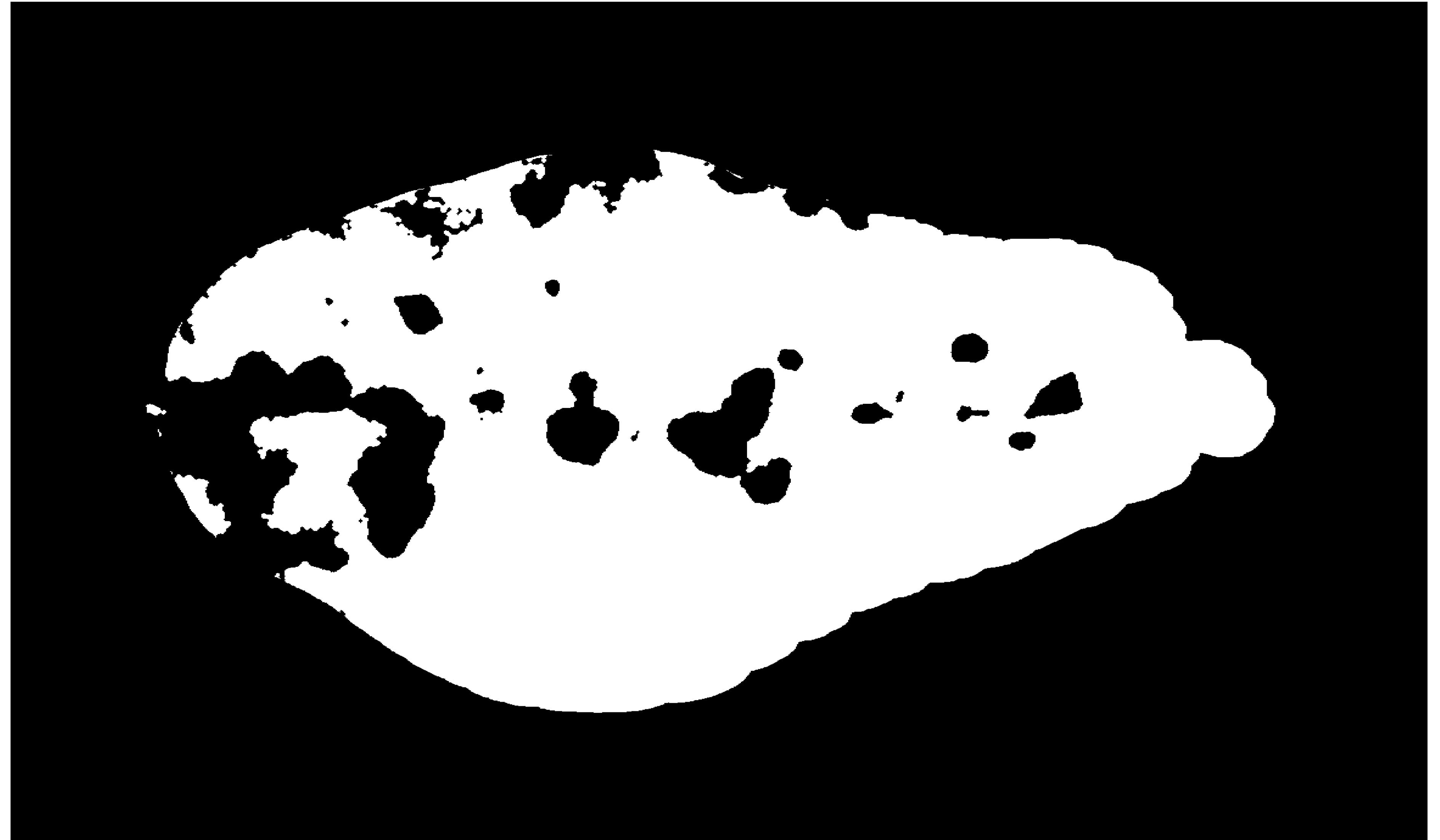
Figure 2. Representative MATLAB-processed binary image of citrus canker symptoms on a lemon leaf at 60 days after inoculation. Image published with permission from the journal Vegetos, Springer Nature, eISSN: 2229-4473.
C. Conversion of RGB image to HSV color space
1. Convert the imported RGB image into HSV color space using the rgb2hsv function.
2. Extract the three HSV channels corresponding to hue (H), saturation (S), and value (V).
3. Store these channels for subsequent segmentation of diseased tissue.
Critical: HSV color space separates chromatic information from brightness and improves discrimination between symptomatic and healthy tissue compared with direct RGB thresholding. This separation facilitates more consistent identification of diseased tissues exhibiting distinct color changes, although segmentation accuracy still depends on image quality and appropriate selection of HSV threshold values.
D. Segmentation of diseased tissue using HSV thresholds
1. Use the HSV channels extracted in section C to identify pixels corresponding to diseased tissue.
2. Define threshold ranges for the H, S, and V channels that correspond to the color characteristics of necrotic symptomatic regions.
3. Apply the defined threshold conditions to the H, S, and V channels to generate binary masks representing candidate diseased pixels.
4. Combine the binary masks using logical operations to generate a disease mask representing pixels corresponding to symptomatic tissue.
5. Visualize the resulting segmentation output in MATLAB to confirm that the diseased regions are correctly detected.
Note: The HSV threshold values used in this protocol were selected empirically by repeatedly examining representative leaf images acquired under controlled illumination. Multiple threshold combinations were evaluated, and the final values were chosen because they consistently separated visually diseased tissues from healthy tissues while minimizing misclassification of background pixels and healthy leaf regions. The selected threshold values used for disease segmentation are summarized in Table 1. These values were optimized for the representative image dataset used in this study and should therefore be regarded as dataset-specific rather than universally applicable.
Table 1. HSV threshold values used for disease segmentation
| Parameter | Threshold | Purpose |
|---|---|---|
| Hue (H) | 0.05–0.15 | Identifies yellow-brown symptomatic tissues in the representative dataset used in this study. |
| Saturation (S) | >0.20 | Removes weakly saturated pixels and reduces background interference. |
| Value (V) | 0.20–0.85 | Excludes very dark shadowed regions and highly reflective pixels. |
Critical: The HSV threshold values directly influence segmentation accuracy because they determine which pixels are classified as diseased tissue. Threshold values that are too restrictive may exclude genuine lesions (false negatives), whereas overly permissive thresholds may incorrectly classify healthy tissue or background as diseased (false positives). When applying this protocol to different plant species, disease symptoms, imaging systems, or illumination conditions, users should inspect representative images, evaluate the segmentation output visually, and adjust the HSV thresholds as necessary to achieve accurate lesion detection.
E. Morphological refinement of the disease mask
1. Apply morphological opening to the disease mask to remove small isolated pixels resulting from segmentation noise.
2. Apply morphological closing to connect fragmented symptomatic regions belonging to the same lesion.
3. Fill internal holes in the binary disease mask to obtain a continuous representation of necrotic tissue.
4. Display the refined mask in MATLAB to confirm that symptomatic regions are accurately represented.
Note: Morphological opening was performed using a disk-shaped structuring element with a radius of 2 pixels to remove small isolated pixels and segmentation noise while preserving lesion boundaries. Morphological closing was subsequently performed using a disk-shaped structuring element with a radius of 4 pixels to connect fragmented lesion regions and smooth small discontinuities within the segmented diseased tissue. These parameter values were selected empirically using representative images from the present study and provided consistent refinement of the disease mask. Depending on image resolution, lesion size, and image quality, users may adjust the structuring element size to optimize segmentation performance.
Critical: The size of the structuring element directly influences the refinement process. Excessively large structuring elements may remove small lesions or merge adjacent lesions, whereas very small structuring elements may fail to remove segmentation noise. Users should visually inspect the refined disease mask before proceeding to disease-area calculation and adjust the structuring element size if necessary.
F. Extraction of total leaf area
1. Convert the original RGB image into grayscale using the MATLAB function rgb2gray.
2. Apply automatic thresholding using the graythresh function to separate the leaf from the background.
3. Convert the thresholded grayscale image into a binary mask representing the entire leaf area.
4. Fill holes in the binary mask to ensure that the leaf area forms a continuous region.
5. Apply morphological opening to remove background noise that may appear in the binary mask.
6. Display the resulting leaf mask to verify that the entire leaf surface has been correctly segmented.
Critical: Accurate leaf segmentation requires sufficient contrast between the leaf surface and the surrounding background. Images with complex or similarly colored backgrounds may require adjustment of the segmentation parameters.
G. Differentiation of healthy and diseased tissue
1. Use the refined disease mask obtained in section E and the total leaf mask obtained in section F to distinguish between healthy and diseased regions.
2. Subtract the disease mask from the leaf mask to obtain the healthy leaf region.
3. Display the resulting binary image showing the spatial distribution of healthy and diseased tissues.
4. Verify visually that necrotic regions have been correctly classified as diseased pixels and that the remaining pixels correspond to healthy leaf tissue.
Critical: Errors in either disease segmentation or leaf segmentation may affect the final classification of healthy and diseased tissues. Before proceeding to area calculation, visually compare the binary classification image with the original RGB image to confirm that symptomatic regions have been correctly identified and that healthy leaf tissues and background pixels have not been incorrectly classified.
H. Calculation of diseased area percentage
1. Count the number of pixels corresponding to diseased tissue using the refined disease mask.
2. Count the total number of pixels representing the entire leaf area using the leaf mask.
3. Calculate the percentage of diseased area using the following formula:
Disease percentage = (number of diseased pixels / total number of leaf pixels) × 100
4. Display the calculated values for diseased area, total leaf area, and percentage diseased area in the MATLAB Command Window.
Expected outcome: The workflow generates (i) the original RGB leaf image, (ii) the final binary image showing the differentiated healthy and diseased tissues, and (iii) quantitative measurements of diseased area (pixels), total leaf area (pixels), and percentage diseased area displayed in the MATLAB Command Window. Before accepting the calculated disease percentage, users should visually verify that the segmented diseased regions correspond closely to the symptomatic tissues in the original image. A representative MATLAB interface and output generated using the workflow are shown in Figure 3.
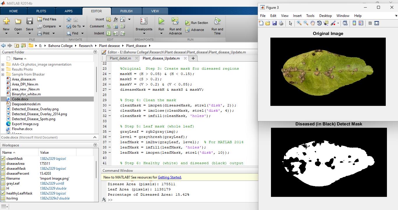
Figure 3. Representative MATLAB interface showing implementation of the hue-saturation-value (HSV)-based disease segmentation workflow. The interface displays the original RGB leaf image, the corresponding binary disease mask, and the quantitative outputs, including diseased area, total leaf area, and percentage diseased area calculated by the workflow.
MATLAB code used for image processing and disease quantification
The MATLAB script used to perform image loading, HSV conversion, disease segmentation, mask refinement, leaf area extraction, and pixel-based disease quantification is provided below.
Note: The following MATLAB script implements the complete workflow described above, including image import, RGB-to-HSV conversion, HSV thresholding, morphological refinement, leaf segmentation, and pixel-based disease area calculation. The script was developed and tested using MATLAB R2014b together with the Image Processing Toolbox.
clc;clear;% Step 1: Load the image[filename, pathname] = uigetfile({'*.jpg;*.png;*.jpeg'}, 'Select an Image');img = imread(fullfile(pathname, filename));figure, imshow(img), title('Original Image')% Step 2: Convert to HSVhsvImg = rgb2hsv(img);H = hsvImg(:,:,1);S = hsvImg(:,:,2);V = hsvImg(:,:,3);% Step 3: Create mask for diseased regionsmaskH = (H > 0.05) & (H < 0.15);maskS = (S > 0.2);maskV = (V > 0.2) & (V < 0.85);diseaseMask = maskH & maskS & maskV;% Step 4: Clean the maskcleanMask = imopen(diseaseMask, strel('disk', 2));cleanMask = imclose(cleanMask, strel('disk', 4));cleanMask = imfill(cleanMask, 'holes');% Step 5: Leaf mask (whole leaf)grayLeaf = rgb2gray(img);level = graythresh(grayLeaf);leafMask = im2bw(grayLeaf, level);leafMask = imfill(leafMask, 'holes');leafMask = imopen(leafMask, strel('disk', 10));% Step 6: Healthy leaf maskhealthyLeafMask = leafMask & ~cleanMask;% Step 7: Display resultsfigure;imshow(img);title('Original Leaf Image');figure;imshow(healthyLeafMask);title('Diseased (in Black) Detect Mask');% Step 8: Save outputimwrite(healthyLeafMask, 'Healthy_vs_Diseased_BW.png');% Step 9: Area calculationdiseaseArea = sum(cleanMask(:));leafArea = sum(leafMask(:));fprintf('Disease Area (pixels): %d\n', diseaseArea);fprintf('Leaf Area (pixels): %d\n', leafArea);if leafArea > 0 diseasePercent = (diseaseArea / leafArea) * 100;else diseasePercent = 0;endfprintf('Percentage of Diseased Area: %.2f%%\n', diseasePercent);Critical: The HSV threshold values used in this script correspond to the representative image dataset used in this study. When applying the workflow to different plant species, disease symptoms, image resolutions, or illumination conditions, users should visually inspect the segmentation output and adjust the threshold values where necessary to achieve accurate disease segmentation.
Data analysis
The MATLAB script described in this protocol generates quantitative measurements of disease severity from digital leaf images by calculating the number of pixels corresponding to diseased tissue and the total number of pixels representing the leaf area. The percentage of diseased tissue is calculated using the following equation:
Disease percentage = (diseased pixels/total leaf pixels) × 100
Each analyzed image represents one observational unit, typically corresponding to a single leaf. When multiple leaves are assessed within the same experimental unit (e.g., plant or treatment replicate), the calculated disease severity values may be averaged to obtain a representative estimate for that unit. Before statistical analysis, users should visually verify that the segmentation output accurately represents the symptomatic regions in each image and exclude images with obvious segmentation errors from further analysis.
The resulting disease severity values can be used for statistical analyses depending on the experimental design employed in the study. In experiments where multiple treatments or genotypes are arranged in designs such as completely randomized design (CRD) or randomized block design (RBD), treatment effects can be evaluated using analysis of variance (ANOVA). If significant differences are detected, post hoc multiple comparison tests such as Tukey’s honest significant difference test may be used to determine pairwise differences among treatments. In experiments comparing only two groups, statistical differences in disease severity may be evaluated using Student’s t-test. When disease severity is measured across multiple time points to evaluate disease progression, the data can be analyzed using two-way ANOVA, repeated-measures ANOVA, or mixed-effects models, depending on the structure of the experimental replication and the sampling design.
Before performing statistical tests, it is advisable to examine the dataset for normality and homogeneity of variance. Percentage disease severity data may be analyzed directly when the assumptions of parametric tests are satisfied. If these assumptions are violated, appropriate data transformation, such as the arcsine square-root transformation, may be performed before statistical analysis. Following statistical analysis, graphical visualization of disease severity data facilitates the interpretation of treatment effects and temporal disease development. Visualization methods may include bar plots displaying mean disease severity across treatments with associated variability measures such as standard error, box plots illustrating the distribution of disease severity among replicates, and line graphs representing disease progression across time points.
These statistical analyses and graphical visualizations can be performed using several commonly used statistical software platforms. For example, the R statistical environment allows analysis of variance to be performed using the aov() function, while post hoc comparisons may be conducted using functions such as TukeyHSD() or functions available in packages such as agricolae. Data manipulation and organization can be carried out using packages such as dplyr, and graphical visualization can be generated using ggplot2, which provides flexible tools for producing bar plots, box plots, and line graphs suitable for publication. Similar analyses may also be performed using other statistical software such as SPSS, GraphPad Prism, Python-based statistical environments, or Origin. The choice of statistical methods and visualization approaches should be determined based on the experimental design, number of treatments, and the objectives of the study.
Validation of protocol
The reliability of this protocol was validated through its application in controlled experiments evaluating disease progression on citrus leaves. The protocol was used to quantify symptomatic tissue by distinguishing necrotic lesions from healthy leaf regions using HSV-based image segmentation and pixel-based area calculations. In the validation study, leaf images were collected from multiple plants subjected to different experimental treatments and time points. The MATLAB-based image processing pipeline successfully generated consistent segmentation outputs that allowed quantitative comparison of disease severity across treatments. The resulting measurements were subsequently used for statistical analysis of disease incidence, disease severity, and treatment efficacy. The segmentation outputs generated by the MATLAB workflow correspond to the MATLAB-processed images presented in Figure 2, which illustrate the differentiation between healthy and diseased tissue regions following image analysis. These outputs demonstrate the ability of the protocol to reliably identify symptomatic regions and quantify disease severity based on pixel-based measurements. The protocol was developed and optimized using representative images of citrus canker symptoms acquired under standardized imaging conditions. The representative example presented here is intended to demonstrate the workflow rather than to establish universal segmentation performance across different plant species or disease types.
This protocol (or parts of it) has been used and validated in the following research article:
• Purkayastha et al. [8]. Zinc-based nutritional antimicrobials as a dual-action strategy against Xanthomonas citri in Citrus limon. Vegetos (Figures 2 and 3).
The successful application of this method in experimental disease evaluation demonstrates that the protocol provides a reproducible and objective approach for quantifying plant disease severity from digital leaf images. The accuracy of the workflow depends on image quality, symptom visibility, and the appropriate selection of HSV threshold values. When the protocol is applied to different plant species, disease symptoms, imaging systems, or illumination conditions, users should verify the segmentation results visually and adjust the HSV threshold values where necessary before quantitative analysis.
General notes and troubleshooting
General notes
1. The accuracy of disease segmentation in this protocol depends strongly on the contrast between diseased and healthy tissue in the captured images. Symptoms that produce clear visual differences in color or texture relative to healthy tissue are most suitable for analysis using the HSV-based segmentation approach described here. Diseases that do not produce distinct visual symptoms or that cause very subtle discoloration may require adjustment of segmentation thresholds or alternative image analysis methods.
2. Image acquisition conditions influence the performance of the segmentation algorithm. Variations in lighting intensity, shadow formation, or reflections on the leaf surface may alter color values in the image and affect threshold-based detection of diseased regions. To minimize variability, it is recommended to capture all images under consistent illumination conditions and with a similar camera orientation and distance from the leaf surface.
3. The threshold values used for HSV segmentation may require adjustment when applying the protocol to different plant species, diseases, or imaging environments. Differences in lesion coloration, background color, and camera settings can influence the HSV ranges corresponding to symptomatic tissue. Preliminary inspection of sample images and testing of threshold ranges may be necessary when adapting the protocol to new experimental systems.
4. The protocol is applicable to a wide range of plant diseases in which symptomatic regions can be visually distinguished from healthy tissue. This includes diseases producing necrotic lesions, blight symptoms, or other clearly discolored regions. The approach can therefore be adapted to various host–pathogen systems, provided that the symptomatic regions exhibit sufficient visual contrast relative to the surrounding healthy tissue.
5. The segmentation approach used in this protocol is based on pixel classification and therefore provides relative measurements of diseased area rather than absolute physical area unless a spatial scale reference is included during image acquisition. If absolute measurements of lesion size are required, a scale marker can be included in the image during photography and used for spatial calibration.
6. The workflow is intended for plant diseases that produce visually distinguishable symptoms under reasonably controlled imaging conditions. When applying the protocol to different plant species, disease symptoms, image resolutions, or illumination conditions, optimize the HSV threshold values and visually verify the segmentation output before quantitative analysis.
Troubleshooting
Problem 1: Diseased regions are not correctly detected in the segmented output image.
Possible cause: The HSV threshold values used for segmentation do not correspond to the color characteristics of the disease symptoms in the analyzed images.
Solution: Adjust the HSV threshold ranges used in the segmentation step by examining the color values of symptomatic regions in the image and modifying the threshold parameters accordingly.
Problem 2: Healthy tissue is incorrectly classified as diseased tissue.
Possible cause: Variations in illumination or background color may produce pixel values similar to those of symptomatic regions.
Solution: Capture images under uniform lighting conditions and avoid backgrounds with colors similar to the leaf surface. Adjust HSV threshold values to better discriminate between healthy and diseased tissue.
Problem 3: The leaf area is not correctly segmented from the background.
Possible cause: Insufficient contrast between the leaf surface and the background in the captured image.
Solution: Capture images against a background that contrasts clearly with the leaf surface or adjust the grayscale threshold used during leaf mask generation.
Problem 4: Small lesions are removed during morphological processing.
Possible cause: The structuring element used in morphological operations may be too large, causing removal of small symptomatic regions.
Solution: Reduce the size of the structuring element used during morphological opening or closing to preserve smaller lesions while still removing noise artifacts.
Problem 5: Diseased tissue is substantially over-segmented or under-segmented.
Possible cause: The selected HSV threshold values are not suitable for the symptom color, image resolution, camera settings, or illumination conditions of the analyzed image.
Solution: Compare the segmented output with the original RGB image and adjust the hue, saturation, and value threshold ranges incrementally until the visible symptomatic regions are adequately detected with minimal classification of healthy tissue or background. If satisfactory segmentation cannot be achieved, reacquire the image under more uniform illumination or exclude it from quantitative analysis.
Acknowledgments
Bhaskar Dowarah and Pankaj Borah contributed equally to this work. Conceptualization, B.D., P.B.; Investigation, B.D., P.B., A.K., B.N.; Software and MATLAB coding, P.B.; Writing—Original Draft, B.D.; Writing—Review & Editing, B.D., P.B., R.A.L., A.K., B.N., A.Y.; Supervision, B.N., A.K.
This research received no external funding.
This protocol was described and validated in Purkayastha et al. [8].
The graphical overview and schematic illustrations presented in this protocol were created using Adobe Illustrator (Adobe Inc., San Jose, California, USA).
Competing interests
The authors declare that they have no financial or non-financial competing interests related to this work. The authors confirm that they have no affiliations with or involvement in any organization or entity with any financial interest (such as employment, consultancy, stock ownership, patent applications, or funding) or non-financial interest (such as personal or professional relationships) that could have influenced the work reported in this manuscript.
Ethical considerations
This study does not involve human participants, animals, or clinical trials. Therefore, ethical approval and informed consent were not required. All experiments were conducted in accordance with standard laboratory biosafety and research guidelines.
References
- Bock, C. H., Poole, G. H., Parker, P. E. and Gottwald, T. R. (2010). Plant Disease Severity Estimated Visually, by Digital Photography and Image Analysis, and by Hyperspectral Imaging. Crit Rev Plant Sci. 29(2): 59–107. https://doi.org/10.1080/07352681003617285
- Nutter, Jr., F. W. (1993). Assessing the Accuracy, Intra-rater Repeatability, and Inter-rater Reliability of Disease Assessment Systems. Phytopathology. 83(8): 806–812. https://doi.org/10.1094/phyto-83-806
- Bock, C. H., Parker, P. E., Cook, A. Z. and Gottwald, T. R. (2008). Visual Rating and the Use of Image Analysis for Assessing Different Symptoms of Citrus Canker on Grapefruit Leaves. Plant Dis. 92(4): 530–541. https://doi.org/10.1094/pdis-92-4-0530
- Mahlein, A. K. (2016). Plant Disease Detection by Imaging Sensors – Parallels and Specific Demands for Precision Agriculture and Plant Phenotyping. Plant Dis. 100(2): 241–251. https://doi.org/10.1094/pdis-03-15-0340-fe
- Meyer, G. E., Mehta, T., Kocher, M. F., Mortensen, D. A. and Samal, A. (1998). Textural Imaging and Discriminant Analysis for Distinguishing Weeds for Spot Spraying. Trans ASAE. 41(4): 1189–1197. https://doi.org/10.13031/2013.17244
- Gonzalez, R. C. and Woods, R. E. (2018). Digital Image Processing (4th ed.). New York: Pearson Education.
- Schindelin, J., Arganda-Carreras, I., Frise, E., Kaynig, V., Longair, M., Pietzsch, T., Preibisch, S., Rueden, C., Saalfeld, S., Schmid, B., et al. (2012). Fiji: an open-source platform for biological-image analysis. Nat Methods. 9(7): 676–682. https://doi.org/10.1038/nmeth.2019
- Purkayastha, A., Dowarah, B., Kashyap, A., Nath, B. C., Bhattacharyya, P. N., Borah, P., Laskar, R. A. and Neog, B. (2026). Zinc-based nutritional antimicrobials as a dual-action strategy against Xanthomonas citri in Citrus limon. Vegetos.: e1007/s42535–026–01647–1. https://doi.org/10.1007/s42535-026-01647-1
Article Information
Publication history
Received: May 18, 2026
Accepted: Jul 22, 2026
Available online: Aug 5, 2026
Published: Aug 20, 2026
Copyright
© 2026 The Author(s); This is an open access article under the CC BY-NC license (https://creativecommons.org/licenses/by-nc/4.0/).
How to cite
Dowarah, B., Borah, P., Laskar, R. A., Yasin, A., Kashyap, A. and Neog, B. (2026). A MATLAB-Based Image Processing Protocol for Quantitative Differentiation of Diseased and Healthy Plant Tissue From Digital Leaf Images. Bio-protocol 16(16): e5798. DOI: 10.21769/BioProtoc.5798.

 Download Citation in RIS Format
Category
Plant Science > Plant immunity > Disease symptom
Plant Science > Plant physiology > Phenotyping
Bioinformatics and Computational Biology
Do you have any questions about this protocol?
Post your question to gather feedback from the community. We will also invite the authors of this article to respond.
 Post a Question


