


- Protocols

- Articles and Issues
- For Authors
- About
- Become a Reviewer


Engineering MRI-Based Programmable Genetic Sensors Using the MAPPER Platform

Published: Vol 16, Iss 17, Sep 5, 2026 DOI: 10.21769/BioProtoc.5795 Views: 185
Reviewed by: Gundeep KaurAnonymous reviewer(s)
 PDF
PDF  Ask a question
Original research article
The authors used this protocol in:

Jan 2026
Advertisement


Protocol Collections
Comprehensive collections of detailed, peer-reviewed protocols focusing on specific topics




Abstract
Genetically encodable reporters that produce signals detectable in deep tissues offer a powerful tool for noninvasive monitoring of molecular events in vivo. Although magnetic resonance imaging (MRI) is a standard technique for noninvasive clinical imaging, its wider application in detecting molecular activities has been constrained by the lack of programmable sensors. This limitation is in stark contrast to the widespread use of fluorescent reporter–derived sensors in cultured cells and in transparent specimens. To overcome this limitation, we recently developed the modular aquaporin-based protease-activatable probe for enhanced reporting (MAPPER) platform. This sensor engineering framework integrates a metal-free MRI reporter derived from human aquaporin-1 (hAqp1) with synthetic protease-based circuits. This integration facilitates the modular and scalable creation of a wide range of sensors by regulating protease activity through precise molecular events, such as protein–protein interactions, pharmacological inhibition, and second messenger signaling. In this paper, we present a detailed protocol for constructing and deploying sensors using the MAPPER paradigm. The protocol encompasses genetic design, lentiviral production, stable cell line generation, biochemical and microscopic validation of sensor function, diffusion-weighted MRI, and MR image analysis to quantify sensor signals in terms of the apparent diffusion coefficient. We describe two distinct MAPPER architectures: DD-MAPPER, which leverages protease-controlled protein degradation, and ER-MAPPER, which utilizes protease-controlled, subcellular trafficking. The MAPPER framework allows adaptation to various molecular targets without the need to redesign the core MRI reporter mechanism, making MAPPER a versatile platform for noninvasive biosensing in living cells and tissues.
Key features
• MAPPER enables programmable, protease-controlled switching of aquaporin-1-based diffusion weighted-MRI signals in genetically modified mammalian cells.
• The protocol covers two complementary biosensor architectures (DD-MAPPER and ER-MAPPER) that exploit different post-translational regulatory mechanisms to modulate MRI signals.
• Stable MAPPER cell lines are generated via lentiviral transduction, allowing long-term, selection-free biosensor expression across multiple mammalian cell types.
• The sensor is fully modular; proteases and protease-based logic circuits can be substituted without altering the hAqp1 reporter, enabling rapid adaptation to new molecular targets.
Keywords: MRI Noninvasive biosensors
Aquaporins
Reporter genes
Protease circuits
Diffusion-weighted MRI
Noninvasive biosensors
Aquaporins
Reporter genes
Protease circuits
Diffusion-weighted MRI
Graphical overview
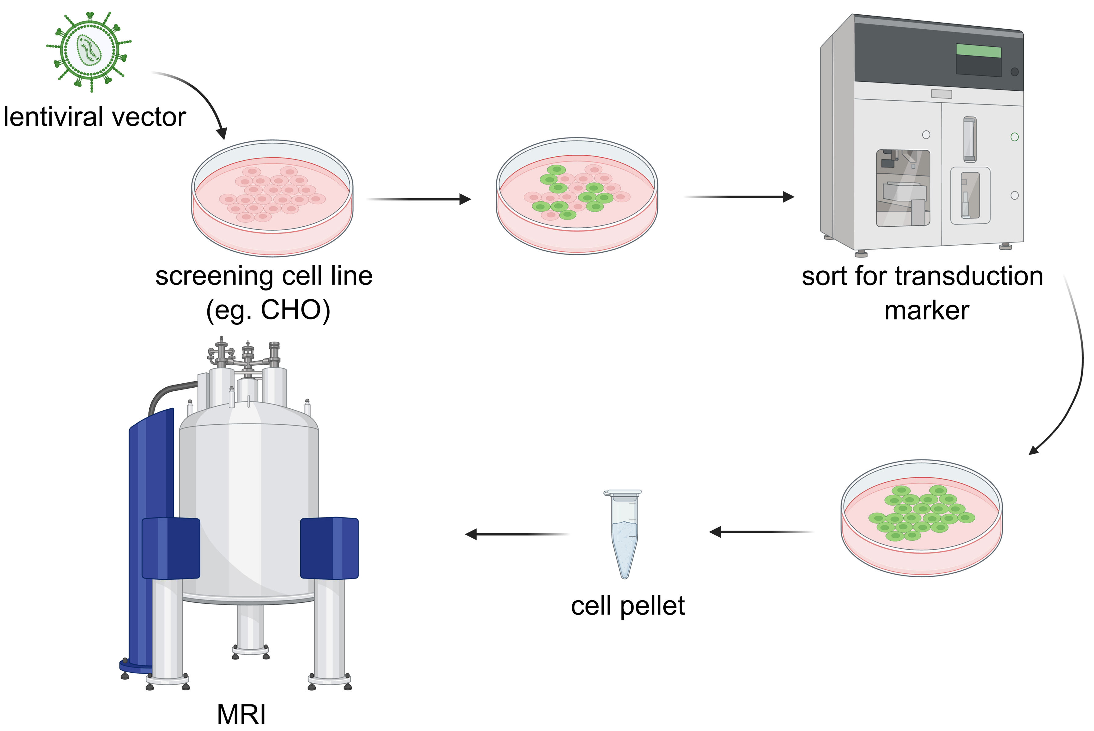
Workflow for generating and imaging MAPPER-expressing cells. CHO cells are stably transduced with lentiviral vectors encoding MAPPER constructs, sorted by fluorescence-activated cell sorting (FACS) to select successfully transduced cells, expanded to confluence, pelleted by centrifugation, and imaged by diffusion-weighted magnetic resonance imaging (MRI). MAPPER: modular aquaporin-based protease-activatable probe for enhanced reporting.
Background
The ability to monitor molecular events in living tissues noninvasively is a long-standing goal of biomedical research [1]. Understanding how diseases such as cancer, neurodegeneration, and inflammation develop at the molecular level requires tools that can report on biological events such as enzyme activation, protein–protein interactions, signaling, and drug action, within intact, optically opaque experimental models. Magnetic resonance imaging (MRI) is uniquely suited to this challenge: it generates high-resolution (from millimeters in humans to ~100 μm in rodents), three-dimensional images of soft tissue without utilizing ionizing radiation and has no depth constraint, making it one of the few modalities compatible with longitudinal molecular imaging in whole animals in both research and clinical settings.
Consequently, the development of genetically encoded reporters that produce detectable MRI signals has been an active area of research for over two decades [2–6]. Genetically encoded reporters for MRI can be broadly categorized by their contrast mechanism: metal-based reporters that alter T1 or T2/T2* relaxation times by accumulating paramagnetic ions, and water-exchange reporters that increase the apparent diffusion coefficient (ADC) of cellular water detectable by diffusion-weighted MRI. The latter is the foundation of the modular aquaporin-based protease-activatable probe for enhanced reporting (MAPPER) platform described in this protocol. Early approaches focused on metalloprotein overexpression by engineering cells to accumulate iron via ferritin or transferrin receptor overexpression, producing local perturbations in T2 or T2* relaxation rates that could be detected using standard T2-weighted imaging protocols similar to blood oxygenation level–dependent functional MRI (BOLD-fMRI) [7–9]. While these reporters have been used successfully in cell-tracking studies, they carry notable limitations. They are constitutively active, signal magnitude depends on expression level rather than on a specific molecular event, and, critically, require exogenous iron supplementation to generate sufficient MRI contrast. Together, these properties make them poorly suited to biosensing applications that require a switchable, activity-dependent readout. A second class of reporters exploits paramagnetic metal-binding proteins, including engineered variants of the dopamine- and serotonin-sensing MRI reporters developed by directed evolution [2], and calcium-responsive reporters based on calprotectin-driven chelation of manganese [10]. These provide genuine biosensing functionality but still require exogenous metal cofactors, limiting their applicability in vivo and raising translational concerns. A third class exploits chemical exchange saturation transfer (CEST), in which highly charged polypeptides, such as polylysine, exchange protons with bulk water at a distinct frequency offset, generating contrast without paramagnetic metals [11]. While promising, CEST reporters suffer from relatively low sensitivity compared to metal-based approaches. More recently, gas vesicle–based acoustic reporters derived from aquatic microorganisms have been developed and shown to function in mammalian cells, offering a distinct and genetically encodable contrast mechanism [12]. However, the large genetic payload required for gas vesicle biosynthesis, combined with the lower depth penetration of ultrasound compared to MRI, constrains their widespread practical deployment.
Aquaporin-based reporters represent a conceptually different and practically attractive strategy. Aquaporins are compact, single-gene transmembrane water channels that accelerate transcellular water exchange, producing a measurable increase in the ADC detectable by diffusion-weighted MRI (DW-MRI), a sequence available on virtually every clinical and preclinical MRI scanner with no exogenous contrast agent required. Human aquaporin-1 (hAqp1) was established as a genetically encoded MRI reporter by our lab in 2016 [5], and subsequent work demonstrated its safety and utility across diverse mammalian cell types [13] and in vivo. Notably, hAqp1 has been used as a gene reporter to track viral delivery across the blood–brain barrier (BBB), trace neural connectivity in the rodent brain, and monitor tumor progression in mice. Despite these advances, a key limitation remained: aquaporin-based reporters lacked a general, modular framework for coupling the reporter to arbitrary molecular inputs. Each new biosensor application required independent engineering of the aquaporin protein itself, with no guarantee that the sensing domain would modulate channel activity as intended.
The MAPPER platform described in this protocol addresses this limitation by decoupling the reporter (hAqp1) from the sensing module [14]. Rather than engineering the aquaporin directly, MAPPER places hAqp1 under the post-translational control of synthetic viral protease circuits, a strategy that exploits the well-characterized programmability of protease-based signaling architectures developed in the synthetic biology field [15,16]. Two complementary mechanisms are provided: DD-MAPPER, in which hAqp1 stability is controlled by a protease-cleavable destabilizing domain (DD) [17–19], and ER-MAPPER, in which hAqp1 membrane trafficking is regulated by a protease-cleavable endoplasmic reticulum retention signal (ER) [20]. Because the protease recognition sequence and not the aquaporin itself is the point of input integration, a new molecular target can be detected simply by rewiring the upstream protease circuit: substituting a different protease, splitting the protease across two interacting proteins to sense protein–protein interactions, or placing protease expression under ligand-dependent post-transcriptional control. This modularity sharply reduces the engineering burden compared with prior reporter strategies and, critically, has been validated across diverse mammalian cell types and multiple target classes without requiring optimization of the core reporter for each application.
One potential limitation of MAPPER-based sensors is the latency associated with protease-based regulation; signal changes reflect cumulative protease activity over several minutes to hours, rather than capturing instantaneous molecular events. This mechanism is similar to that of integral sensors in optical imaging and offers several practical benefits, such as a higher signal-to-noise ratio and applicability in awake, ambulatory animals. Another limitation of MAPPER is the larger genetic footprint of these sensors because of their circuit-based (rather than conventional single protein–based) architecture. Although most MAPPER constructs remain within the packaging limits of lentiviral vectors (~9.2 kb), delivering MAPPERs via adeno-associated viral vectors (AAVs) will likely require splitting the sensor across multiple AAVs for co-transduction. Within this context, it is worth noting that a distinct advantage of MAPPERs is their entirely post-transcriptional operational mechanism, which potentially allows for delivery as mRNA-encoded devices in lipid nanoparticles. This approach circumvents the packaging limitations inherent to viral gene delivery vectors and may be particularly beneficial for the in vivo delivery of gene-based diagnostics, which do not require sustained or permanent genetic modification of cells and tissues.
In summary, the primary advantage of MAPPER over existing MRI reporter technologies is its programmability, offering a sensor engineering platform vis-à-vis a single bespoke biosensor. Beyond the applications demonstrated in the original publication, we anticipate that MAPPER will be useful across a broad biomedical space, from capturing various stages of signal transduction in physiological and disease states to longitudinally tracking the functional outcomes of gene- and cell-based medicines.
Materials and reagents
Biological materials
1. NEB® stable competent E. coli (NEB, catalog number: C3040H)
2. CHO Tet-On® 3G cell line (Clontech, catalog number: 631195)
3. HEK293T (ATCC, catalog number: CRL-3216)
4. pPkg (second-generation lentiviral packaging plasmid, Addgene #12259)
5. pVSV-G (second-generation lentiviral envelope plasmid, Addgene #8454)
6. DD-MAPPER for TEV (Addgene #248354)
7. ER-MAPPER for TEV (Addgene #248355)
8. TEV on inducible CMV Tet ON promoter (Addgene #248360)
Reagents
Cell culture reagents
1. DMEM (4.5 g/L glucose, L-glutamine, sodium pyruvate, phenol red) (Corning, catalog number: MT10013CM)
2. Fetal bovine serum (FBS) (GenClone, catalog number: 25-550)
3. Penicillin-Streptomycin (Pen/Strep) (10,000 U/mL) (Gibco, catalog number: 15140-122)
4. TrypLETM Express Enzyme (1×), phenol red (Gibco, catalog number: 12605-010)
5. PBS (10×, pH 7.4, diluted to 1× in MilliQ water and autoclaved before use) (Apex BioResearch Products, catalog number: 18-244)
6. Sodium butyrate (Thermo Scientific, catalog number: A11079)
7. Polybrene (10 mg/mL, dilute to 8 mg/mL using autoclaved MilliQ water as a 1,000× stock) (Sigma-Aldrich, catalog number: TR-1003-G)
8. Lenti-XTM Concentrator (TaKaRa, catalog number: 631232)
Transfection and cloning reagents
9. LB agar, Miller (Fisher Bioreagents, catalog number: BP1425-500)
10. SOC medium (NEB, catalog number: B9035S)
11. Monarch DNA Gel Extraction kit (NEB, catalog number: T1120L)
12. Ampicillin (GOLDBIO, catalog number: A-301-100)
13. PEI (25 kDa, linear) (Polysciences, catalog number: 23966)
14. Q5® High-Fidelity 2× master mix (New England Biolabs, catalog number: M0492S)
15. PureYieldTM Plasmid Miniprep System (Promega, catalog number: A1223)
16. PureYieldTM Plasmid Midiprep System (Promega, catalog number: A2495)
17. 50× TAE buffer (Thermo Scientific, catalog number: B49)
18. Agarose LE (Goldbio, catalog number: A-201-100)
19. Doxycycline hyclate (Sigma-Aldrich, catalog number: D9891)
20. Gibson assembly master mix; prepared using the protocol described by Miller Lab (https://pengxulab.weebly.com/uploads/7/9/3/5/79359982/gibson_assembly_%E2%80%93_samuel_miller_lab_uw_seattle.pdf)
Chemical reagents
21. 12 M HCl (Sigma-Aldrich, catalog number: 320331-500ML)
22. NaOH (Sigma-Aldrich, catalog number: 881-500G)
23. CuSO4.5H2O (Sigma-Aldrich, catalog number: 939315-100G)
Solutions
1. DMEM complete medium (see Recipes)
2. PEI transfection stock (see Recipes)
3. Sodium butyrate 1 M (see Recipes)
4. Agarose gel (see Recipes)
5. 1% agarose phantom gel with 0.15 g/L CuSO4 (see Recipes)
Recipes
1. DMEM complete medium
| Reagent | Final concentration | Quantity or volume |
|---|---|---|
| DMEM (4.5 g/L glucose, L-glutamine, phenol red) | n/a | 450 mL |
| FBS | n/a | 50 mL |
| Pen/Strep | 10,000 U/mL | 5 mL (100 U/mL) |
Mix all reagents, aliquot into 50 mL tubes, and store at 4 °C until use.
2. PEI transfection stock (0.258 mg/mL, 500 mL)
| Reagent | Final concentration | Quantity or volume |
|---|---|---|
| PEI (25 kDa) | 0.258 mg/mL | 129 mg |
| MilliQ water | n/a | 450 mL |
| 12 M HCl | n/a | As required |
| 10 M NaOH | n/a | As required |
Pour ~450 mL of Milli-Q H2O into a 500 mL glass beaker with stirring. Add 129 mg of linear 25 kDa PEI. Add concentrated HCl dropwise until pH < 2.0 (~800 μL of 12 M HCl). Stir for 2–3 h until PEI is fully dissolved; a small amount of fine fiber particles that do not dissolve is normal and does not affect performance. Add concentrated NaOH dropwise until pH 7.0 (~500 μL of 10 M NaOH). Transfer to a 500 mL glass cylinder and adjust the final volume to 500 mL with MilliQ H2O. Filter-sterilize through a 0.22 μm membrane. Aliquot 10 mL per tube. Store at -20 °C for long-term storage and 4 °C for day-to-day use.
3. Sodium butyrate 1 M, 10 mL
| Reagent | Final concentration | Quantity or volume |
|---|---|---|
| Sodium butyrate | 1 M | 1.1 g |
| MilliQ water | n/a | 10 mL |
Filter-sterilize through a 0.22 μm membrane and store at 4 °C.
4. Agarose gel (for DNA gel electrophoresis)
| Reagent | Final concentration | Quantity or volume |
|---|---|---|
| Agarose | 0.9% w/v | 0.45 g |
| 50× TAE buffer | 1× | 1 mL |
| Deionized water | n/a | 49 mL |
Microwave in 30-s intervals with swirling between each interval, until the solution reaches a full boil, the agarose is completely dissolved, and the solution is clear. Pour into the casting tray with the combs inserted in place. Let the gel form by letting it sit undisturbed for approximately 15–20 min. Remove the comb before use.
5. 1% agarose phantom gel with 0.15 g/L CuSO4 (per 100 mL; adjust to phantom volume)
| Reagent | Final concentration | Quantity or volume |
|---|---|---|
| Agarose | 1% w/v | 1 g |
| CuSO4.5H2O | 0.15 g/L | 15 mg |
| Deionized water | 100 mL |
Combine agarose, CuSO4·5H2O, and deionized water in a heat-resistant flask. Microwave in 30-s intervals with swirling between each interval, until the solution reaches a full boil, the agarose is completely dissolved, and the solution is clear. Pour the solution into the phantom mold before it begins to gel. Once the solution has cooled sufficiently (surface is no longer steaming), place 200 μL PCR tubes into the phantom. Ensure all tubes remain upright throughout cooling.
Critical: Tube tilt at this stage will be permanent once the gel sets, causing systematic errors in MRI ROI placement. Use the weighted phantom stopper (see Equipment) to keep tubes fixed while the gel solidifies. Note that the MRI image will display the mirror image of the physical tube layout.
Pause point: Sealed phantoms can be stored at 4 °C for up to 4 weeks. Inspect for gel cracking, mold growth, or tube drift before each use.
Laboratory supplies
1. 200 μL PCR tubes (Olympus plastics, catalog number: 24-154)
2. 1.5 mL microcentrifuge tubes, sterilized (MBPS Inc., catalog number: MC15-S)
3. Syringe (10 mL) (BD Syringe, catalog number: 309604)
4. 0.22 μm syringe filter (GenClone, catalog number: 25-244)
5. Vacuum bottle top filter (Millipore, catalog number: S2GPT05RE)
6. Aspirating pipettes, 2 mL (Fisherbrand, catalog number: 14-955-135)
7. Serological pipettes 5, 10, and 25 mL (Fisherbrand, catalog numbers: 13-678-11D, 13-678-11E, 13-678-11)
8. 15 and 50 mL conical centrifuge tubes (Thermo Scientific, catalog numbers: 12-565-268, 12-565-270)
9. Tissue culture plates, 10 cm (Fisherbrand, catalog number: FB012924)
10. Tissue culture–treated 6-well plates (Corning, catalog number: 07-200-83)
Equipment
1. Class II Type A2 biosafety cabinet (ThermoFisher Scientific, 1300 series, model: 1377)
2. CO2 incubator, 37 °C, 5% CO2 (ThermoFisher Scientific, model: Forma steri-cycle i160 LK)
3. Refrigerated centrifuge with swing-bucket rotor (ThermoFisher Scientific, catalog number: 75004521)
4. Microcentrifuge/benchtop centrifuge, up to 16,000× g (ThermoFisher Scientific, catalog number: 75002431)
5. Thermocycler for PCR (Applied Biosystems SimpliAmp Thermal Cycler, catalog number: A24812)
6. NanoDrop OneC (Thermo Scientific, catalog number: 13-400-519)
7. Cell sorter (Sony, model: MA900)
8. Diffusion-weighted MRI scanner, Bruker 7 T vertically oriented, actively shielded super-wide bore scanner, 154 mm bore diameter
9. Radiofrequency (RF) probe, 66 mm diameter (MiniSWB90, Bruker, model: 1P T134743)
Software and datasets
1. ImageJ/Fiji, version 2.x (NIH, free; https://imagej.net/software/fiji), used for ROI selection, mean gray value extraction, and basic DW-MRI image processing
2. ParaVision 6.0.1 (Bruker BioSpin, commercial license required; https://www.bruker.com); used for DW-MRI data acquisition and raw image export
3. SnapGene or Benchling (SnapGene: DSBio, commercial; https://www.snapgene.com; Benchling: free for academic use; https://www.benchling.com); used for MAPPER construct design, primer design, and sequence verification
4. MATLAB R2022a Update 4 (version 9.12.0.200938, MathWorks, commercial license required; https://www.mathworks.com); used for ADC fitting and data visualization. The Matlab code used for generating ADC values from the mean grey value and effective b-values has been deposited to GitHub (https://github.com/asishninanchacko-cloud/Bio-Protocols) and archived on Zenodo (https://doi.org/10.5281/zenodo.21045388).
Procedure
A. MAPPER genetic construct design and cloning
A1. Overview of MAPPER construct architecture
MAPPER constructs consist of three modular components assembled in a lentiviral backbone under the human EF1α promoter: (i) the MRI reporter, human aquaporin-1 (hAqp1) with an FLAG epitope tag after Q43; (ii) a 3× protease recognition sequence with GSG linkers in between (here, we will discuss the TEV protease for which the cleavage sequence we used is ENLYFQS, which can be replaced by your protease of interest); and (iii) a regulatory domain; either a destabilizing domain (DD) from FKBP12 or the estrogen receptor ligand-binding domain or Rpn4 (DD-MAPPER), or the ER retention tetrapeptide KKYL (ER-MAPPER).
A2. PCR amplification of insert sequences
Once you design your MAPPER construct with the desired protease cleavage sequence, order the gblock optimized for mammalian cell expression from IDT (or a similar service) with 12–15 bp overlap to the backbone and follow these steps to amplify the backbone.
1. Prepare 25 μL PCR reactions using 2× Q5 high-fidelity master mix: 12.5 μL of 2× Q5 high-fidelity master mix, 1 μL of template plasmid (1–10 ng/μL), 1.25 μL of forward primer (10 μM), 1.25 μL of reverse primer (10 μM), and 9 µL of nuclease-free water.
2. Run the following thermocycler program: 98 °C for 30 s; [98 °C for 10 s, Tanneal for 30 s, 72 °C for 30 s/kb] × 30 cycles; 72 °C for 2 min; hold at 10 °C. Calculate Tanneal using the NEB Tm Calculator (https://tmcalculator.neb.com).
3. Purify PCR products by running a DNA gel (see Recipes) and purifying using the Monarch DNA Gel Extraction kit. Elute in 15 μL of nuclease-free water. Store at -20 °C.
A3. Restriction-free Gibson assembly of MAPPER constructs
Note: This protocol uses a restriction enzyme–free cloning approach. Vector backbone and insert fragments are gel-purified PCR products (section A2). No restriction digestion or DpnI treatment is required prior to assembly.
1. Thaw one 15 μL aliquot of Gibson assembly master mix on ice immediately before use.
2. Add 5 μL of the combined gel-purified DNA fragments (vector + insert at equimolar amounts; 20–200 ng of total DNA) to the 15 μL master mix aliquot (total reaction volume, 20 μL). Mix gently by pipetting 5–6 times. Do not vortex.
3. Incubate at 50 °C for 15–60 min in a thermocycler or heat block. For two-fragment assemblies, 15 min is sufficient; for three or more fragments, incubate for 45–60 min.
4. Place on ice. Transform 1–5 μL of the assembly reaction into 25 μL chemically competent NEB stable cells: add DNA to cells, incubate on ice for 30 min, heat-shock at 42 °C for 30 s, return to ice for 5 min, add 900 μL of SOC medium, shake at 30 °C for 1 h, then plate 150 μL on LB agar with ampicillin (100 μg/mL).
Critical: NEB stable cells must be used instead of standard cloning strains (e.g., DH5α, NEB10β) for propagation of lentiviral transfer vectors. The long terminal repeat (LTR) sequences in the pLenti backbone are prone to recombination and deletion in recA+ strains, which would produce truncated, non-functional constructs that may still yield colonies but fail to produce virus. Grow all cultures containing lentiviral backbone plasmids at 30 °C rather than 37 °C to further minimize recombination.
5. Grow colonies overnight at 30 °C. Pick up to four colonies for miniprep cultures (5 mL LB/ampicillin). Verify insertion by nanopore sequencing.
Critical: Verify the complete coding sequence of hAqp1, the TEVP recognition site, and the DD or KKYL regulatory domain by sequencing before proceeding to lentiviral production.
A4. Endotoxin-free Midiprep for transfection-grade plasmid
1. Inoculate a verified clone into 100 mL LB/ampicillin. Grow at 37 °C and 250 rpm for 20 h.
2. Pellet cells at 5,000× g for 10 min. Purify plasmid using the Promega PureYield Midiprep kit following the manufacturer’s protocol with a vacuum manifold.
3. Elute with 800 μL of nuclease-free water. Measure A260/A280 and A260/A230 on the NanoDrop.
Note: Accept the preparation if A260/A280 > 1.8 and A260/A230 > 2.2.
Pause point: Purified plasmid DNA can be stored at -20 °C indefinitely. Proceed to section B when ready.
B. Lentiviral production and stable cell line generation
B1. HEK 293T cell seeding and transfection for lentiviral packaging
1. Day 0: Seed HEK 293T cells at a 1:6 split ratio from a confluent 10 cm plate into a fresh 10 cm plate containing 10 mL of DMEM complete medium.
2. Day 1: Confirm cells are 70% confluent before transfection. Proceed with PEI-mediated transfection.
Critical: Use HEK 293T cells at passage ≤15 only. Higher passage cells produce significantly lower lentiviral titers.
3. Prepare DNA mix in a 1.5 mL tube: 22 μg of pLenti-MAPPER + 22 μg of pPkg + 4.5 μg of pVSV-G. Bring to 600 μL with 150 mM NaCl. Vortex for 5 s.
4. Prepare PEI mix: 485 μL of PEI stock (0.258 mg/mL) + 115 μL of 150 mM NaCl. Vortex for 5 s.
5. Combine DNA and PEI solutions. Vortex for 10–15 s. Incubate at room temperature for exactly 12 min.
6. Add the 1.2 mL complex dropwise to the HEK 293T plate. Rock gently to distribute. Incubate at 37 °C and 5% CO2.
7. Twenty-four hours post-transfection (hpt), add 100 μL of 1 M sodium butyrate to the existing medium (final concentration 10 mM). Do not aspirate the medium.
Note: Sodium butyrate is a histone deacetylase inhibitor that substantially increases lentiviral yields. Do not exceed 10 mM or add before 24 hpt, as higher concentrations are cytotoxic to HEK 293T cells.
B2. Viral supernatant collection and concentration
1. Seventy-two hours post-transfection, collect the entire spent medium from the plate. Centrifuge at 500× g for 10 min at 4 °C. Transfer the clarified supernatant to a fresh 15 mL tube. Store on ice or at 4 °C.
2. Add 1 volume Lenti-X concentrator to 3 volumes viral supernatant (e.g., 3 mL of Lenti-X to 9 mL of supernatant). Mix gently by inversion.
3. Incubate the tube upright at 4 °C for 24 h.
4. Centrifuge at 1,500× g for 45 min at 4 °C. An off-white pellet should be visible at the tube bottom.
5. Aspirate and discard the supernatant completely. Resuspend the pellet in 1/100th of the original supernatant volume (typically 90–100 μL) of DMEM complete medium or PBS using gentle pipetting. Do not vortex.
6. Aliquot 25 μL per tube. Store at -80 °C. Use within 6 months. Avoid repeated freeze-thaw cycles.
B3. Lentiviral transduction of target cell lines (spinfection method)
1. Seed target cells at multiple densities to ensure 40%–50% confluence at the time of transduction. For CHO cells, use 1:16, 1:8, and 1:6 splits across three wells of a 6-well plate. Add 2 mL of DMEM complete medium per well.
2. Preheat the tissue culture room tabletop centrifuge to 30 °C by spinning at 2,500 rpm for at least 90 min before spinfection.
3. Prepare the transduction mixture in a 1.5 mL tube: 25 μL of concentrated virus + DMEM complete medium to a total volume of 800 μL + 1 μL of 1,000× polybrene stock (8 mg/mL, final concentration 8 μg/mL). Mix gently.
4. Aspirate medium from the target cell well. Add the 800 μL transduction mixture to one well of the 6-well plate.
5. Centrifuge the 6-well plate at 1,050× g at 30 °C for 90 min.
Critical: Centrifuging virus and cells together concentrates viral particles at the cell surface and dramatically increases transduction efficiency, particularly at low multiplicity of infection (MOI). Preheating the centrifuge to 30 °C prevents cold-shock-induced cell death.
Note: Lentiviral titer was not measured in this protocol. Instead, we used a fixed volume of concentrated viral supernatant per transduction well, prepared from a standardized plasmid input (22 μg of transfer plasmid per 10 cm plate of HEK 293T cells), and we used the same gating strategy in FACS between constructs to ensure the same transduction levels. To maximize transduction efficiency and ensure robust overexpression of MAPPER constructs, 25 μL of virus prepared at the end of section B2 was used per well. If transduction efficiency, assessed by fluorescence microscopy at 48 h post-transduction, is less than 20%, discard the viral stock and repeat lentiviral production with freshly transfected HEK 293T cells. At this step, remaking the virus from a different plasmid picked at step A3.5 often proved more effective.
6. Return the plate to the 37 °C, 5% CO2 incubator for 48 h without changing medium.
7. After 48 h, add 200 μL of TrypLE to lift all cells from the transduced well. Resuspend in 10 mL of DMEM complete medium. Seed into a fresh 10 cm plate. Allow cells to expand for 5–7 days with regular medium changes.
8. Sort the cells for fluorescence using fluorescence-activated cell sorting.
Note: Use Figure 1 as a guide for the gate parameters; for a three-color sort, sort efficiency for single-cell sorting (up to 100 cells per well) is higher than 95%.
9. Confirm stable MAPPER expression by western blot for FLAG-hAqp1 before proceeding to MRI experiments.
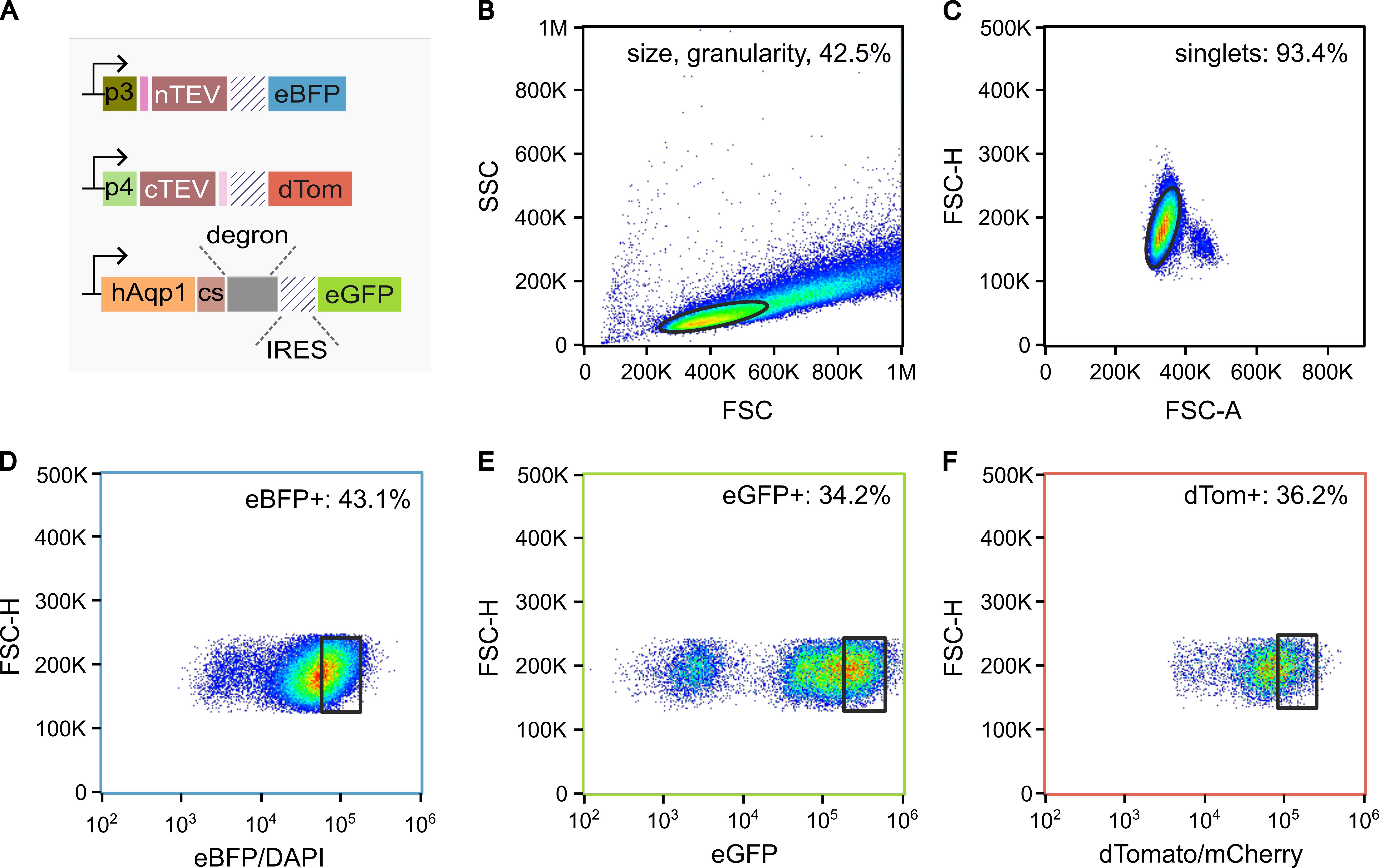
Figure 1. Representative gating strategy for three-color fluorescence-activated cell sorting (FACS) of triply transduced MAPPER cells. (A) Live cells are first selected by size and granularity, followed by singlet discrimination to exclude doublets. (B–F) Fluorescence gates are then applied sequentially for EBFP, dTomato, and EGFP to identify cells stably expressing all three constructs. The MAPPER sensor construct (EGFP) is always transduced last, and the final sort is performed while maintaining the gates established for the previously sorted EBFP and dTomato populations (adapted from Chacko et al. [14], Science Advances, used under CC BY-NC 4.0.). MAPPER: modular aquaporin-based protease-activatable probe for enhanced reporting.
Note: Only use transduced cells for approximately 4 weeks from thaw. Lentiviral expression from stable integrants typically remains stable for this period; prolonged culture may reduce expression due to epigenetic silencing. Prepare 3–5 cryostocks after initial expansion. If you are using the TEV sensor, make sure to transduce the cells with the TEV sensor (Addgene #248360) using the same protocol before transducing with MAPPER. TEV expression needs to be turned on a day before sorting by adding 5 μg/mL doxycycline. Each time a new construct is introduced, cells must be re-sorted for all fluorescent selection markers to confirm stable multi-transgene expression before proceeding to MRI experiments. Serial transductions are recommended as opposed to co-transductions. Western blot for the construct with and without TEV must show a difference in intensity of the bands as well as a change in size. Representative western blots can be found in the original article [14].
C. High-density polyethylene (HDPE) cell pellet phantom fabrication and agarose gel preparation
C1. Phantom design and fabrication
The cell pellet phantom described in this protocol has been developed in the Mukherjee laboratory, optimized for reproducible, high-throughput DW-MRI of cell pellets in PCR tubes. All phantom components are precision-milled from HDPE. HDPE is the material of choice because it is MRI-compatible, produces no MRI signal, is chemically inert to agarose and biological buffers, autoclavable, and dimensionally stable under repeated use.
The phantom consists of three components: an outer cylindrical holder, a molding disc, and a weighted phantom stopper.
1. The outer holder has an outer diameter of 38 mm, sized to fit within the RF volume coil used for imaging (see Equipment). The inner cavity accommodates the molding disc and provides the agarose bath surrounding the PCR tubes during MRI.
2. The molding disc is a circular HDPE disc that seats at the top of the holder cavity via a lip at its perimeter. The disc contains an array of through-holes sized to accept standard 200 μL PCR tubes. Well depth is optimized to approximately twice the height of a PCR tube to ensure full tube support and prevent tilting. Multiple disc layouts are available depending on experimental throughput requirements: 9-hole, 13-hole, and 19-hole configurations are available, with hole placement designed to break radial symmetry so that each tube position is uniquely identifiable in the MRI image. Tube registration between scan sessions is achieved by recording the tube layout diagram at phantom loading (see step D10).
3. The phantom stopper is a weighted HDPE component that sits on top of the molding disc during agarose casting. It keeps PCR tubes fixed in an upright position while the agarose cools and solidifies, preventing tube tilt artifacts that would otherwise be permanent once the gel sets. The stopper is also used during MRI scans to prevent movements during the scan. Contact the corresponding author for technical drawings and fabrication specifications.
Note: The phantom components can be fabricated by 3D printing as an alternative to HDPE milling for laboratories without access to a machine shop. We recommend printing in HDPE filament or, as a widely available alternative, polylactic acid (PLA), both of which are MRI-compatible and produce no detectable signal under the acquisition parameters described in this protocol. All dimensions required for machining or 3D printing the phantom components are provided in Figure 2, and a schematic of the displacement casting and phantom assembly is provided in Figure 3.
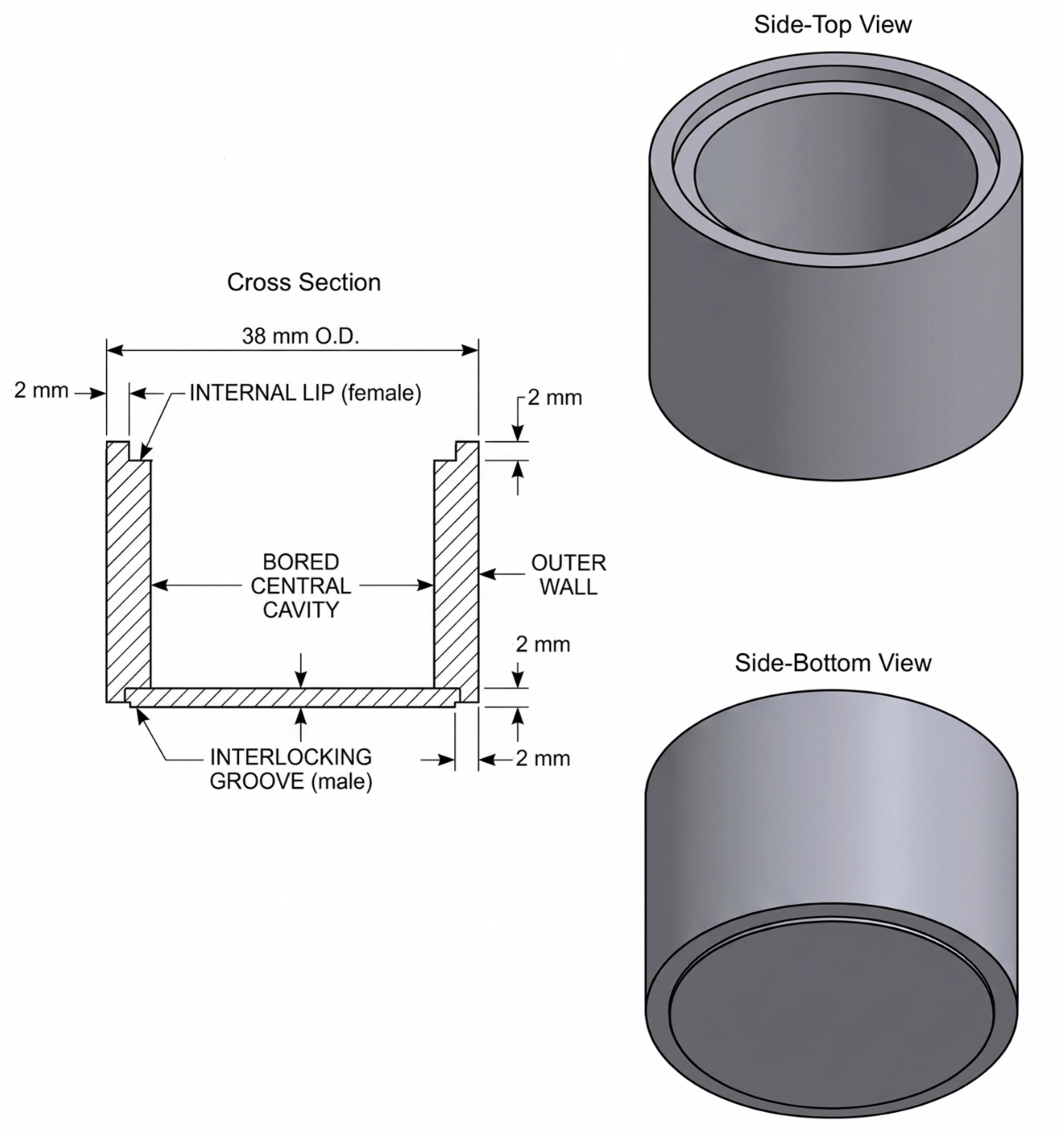
Figure 2. Technical views of the magnetic resonance imaging (MRI) phantom holder. Detailed schematic illustrating the modular high-density polyethylene (HDPE) cylindrical unit. The cross-sectional view (left) highlights the solid wall hatching and the dual-purpose internal top lip. The isometric top and bottom views (right) show the 38-mm outer diameter (O.D.) geometry and the internal bored cavity optimized for agarose displacement and thermal stability.
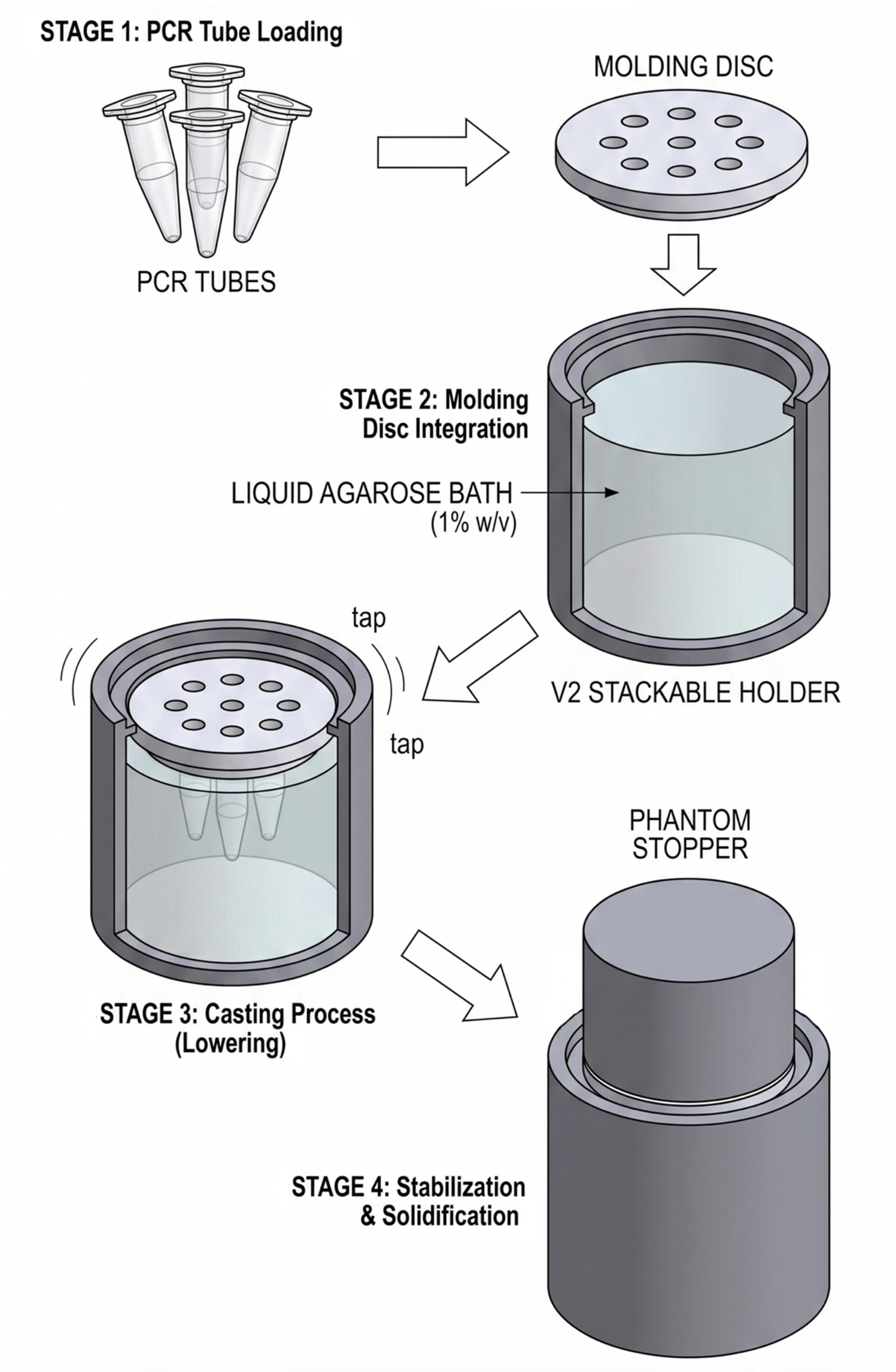
Figure 3. Sequential schematic of the displacement casting and phantom assembly. The modular system is integrated through a four-stage process to ensure a bubble-free imaging matrix. (Stage 1) PCR tubes (0.2 mL) are pre-loaded into the high-density polyethylene (HDPE) molding disc matrix until the tube caps sit flush against the disc surface. (Stage 2) The stackable holder is filled with liquid 1% (w/v) agarose. (Stage 3) The disc-tube assembly is lowered into the holder; the downward displacement forces liquid agarose up around the tubes, while the disc is securely seated on the internal top lip. Mechanical tapping is applied to mitigate air artifacts. (Stage 4) The weighted phantom stopper is positioned on the top unit to stabilize the assembly and fix the vertical orientation of the tubes during the solidification phase.
C2. Agarose gel preparation and phantom casting
Note: Pre-made phantoms stored in the cold room can be reused for up to 4 weeks. If a pre-made phantom with intact gel is available, proceed directly to section E.
1. Calculate the total gel volume required based on the inner dimensions of the phantom holder. Prepare 20% excess volume to account for cooling shrinkage and spillage. Combine agarose (1% w/v) and CuSO4·5H2O (0.15 g/L) in deionized water (see Recipes). Microwave in 30-s intervals with swirling between intervals, until the solution reaches a full boil and is completely clear.
2. Remove from heat. Allow the solution to cool to approximately 50–55 °C with occasional stirring to prevent premature solidification. Monitor temperature with a thermometer.
3. Before pouring, place the molding disc into the holder and insert placeholder 200 μL PCR tubes into each well to reserve tube positions. Ensure all tubes are fully upright and seated at the correct depth.
Critical: Placeholder tubes must be in place before pouring. Attempting to insert tubes into partially set agarose will disturb the gel and create air pockets around the tubes.
4. Pour the cooled agarose slowly into the phantom holder until the gel level reaches just below the top of the molding disc. Avoid introducing air bubbles; remove any surface bubbles with a pipette tip before the gel begins to set.
5. Place the weighted phantom stopper on top of the molding disc to hold the placeholder tubes fixed and upright while the gel cools.
6. Allow the phantom to cool at room temperature for 20–30 min, then transfer to 4 °C for at least 1 h to fully solidify the gel.
7. Remove the phantom stopper and placeholder tubes. The phantom is now ready for loading with cell pellet tubes.
Pause point: Sealed phantoms can be stored at 4 °C for up to 4 weeks. Inspect for gel cracking, mold growth, or tube position drift before each use.
D. Mammalian cell pellet preparation and loading into the phantom
1. Grow MAPPER-expressing cells (on-state and off-state conditions, plus appropriate controls) in separate 10 cm plates to 80%–90% confluence.
2. If you are expressing TEV from a CMV Tet ON promoter, add 5 μL of 10 mg/mL doxycycline (final concentration of 5 μg/mL) to the on-state cells, 24 h prior to the MRI.
3. Wash cells with 4 mL of PBS (leave PBS on cells for 2 min per wash to remove residual serum). Aspirate PBS. Add 1 mL of TrypLE and incubate at 37 °C for 5 min. Tap the plate 3–4 times to dislodge cells.
4. Inactivate trypsin with 9 mL of DMEM complete medium. Triturate gently 4–6 times. Transfer to a 15 mL centrifuge tube.
5. Pellet cells at 350× g for 5 min at room temperature. Aspirate medium completely.
6. Wash the cell pellet with 2 mL of PBS. Centrifuge at 350× g for 5 min. Aspirate supernatant.
7. Resuspend the cell pellet gently in 150 μL of PBS per sample.
Note: One full plate of 90% confluent CHO cells would give you enough cells for a single pellet in a 200 μL PCR tube.
8. Transfer the PBS/cell resuspension to a 200 μL PCR tube per condition.
9. Place PCR tubes in a PCR tube rack that fits your centrifuge rotor. Centrifuge at 500× g for 5 min to form a compact cell pellet at the bottom of each tube.
10. Load the PCR tubes containing cell pellets into the agarose phantom. Record the position of each tube carefully.
Critical: MRI will produce a mirror image of the physical layout (Figure 4). Include a labeled diagram of tube positions in your lab notebook. Complete steps D8 onward as quickly as possible and proceed immediately to MRI acquisition. Cell pellets should not be left at room temperature for more than 30 min before scanning, as cell death and metabolic changes alter ADC values.
11. Seal the phantom top with the molding disc and, if available, the phantom stopper to secure PCR tube positions during transport to the MRI scanner. Protect the whole setup from movements using a paper tape. Then, attach the phantom to a plastic cylinder of the same diameter using a paper tape and insert it into the MRI bore for scanning.
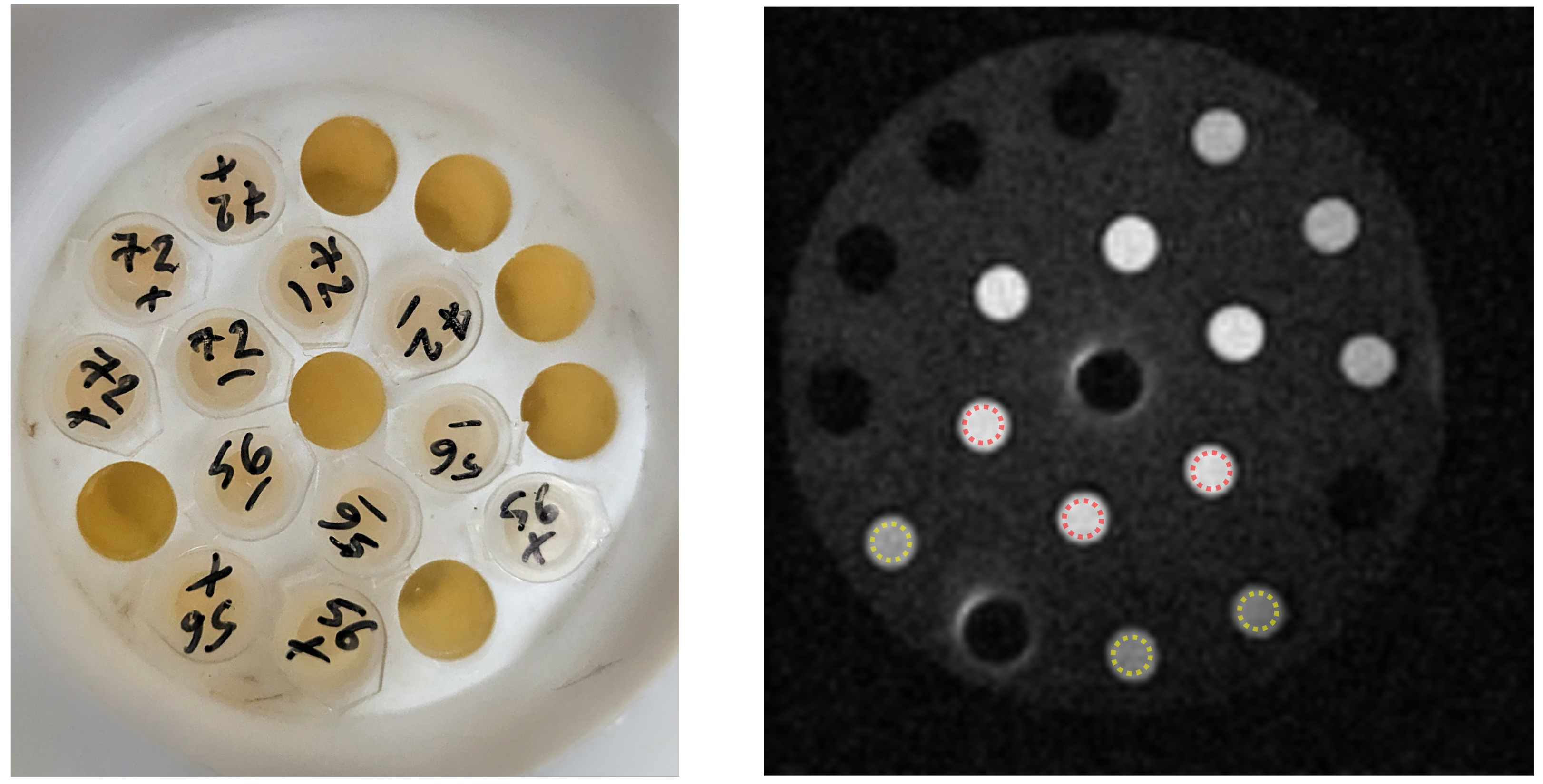
Figure 4. Magnetic resonance imaging (MRI) images. Mirror image (right) of the pellets arranged in the phantom (left). The regions of interest (ROIs) in the MRI image in red are the tubes labeled “56-” in the phantom, and the yellow ROIs are “56+.”
E. Diffusion-weighted MRI acquisition
1. Contact your institutional MRI core facility well in advance to schedule scanner time and discuss the DW-MRI protocol. Provide the phantom dimensions and confirm bore compatibility (the standard phantom tube, outer diameter 40 mm, fits in a standard small-animal MRI volume coil; a phantom of 38 mm diameter is used for cell pellets).
Critical: Temperature critically affects the apparent diffusion coefficient of water in biological samples. Acquire all MRIs at a constant temperature.
2. Acquire DW-MRI data using a stimulated echo (STE) sequence. Recommended parameters are shown in Table S1. Consult scanner documentation for equivalent sequence names.
3. Export DW-MRI images in DICOM format for offline analysis (section F).
Note: Acquire a scout/localizer image first to confirm phantom orientation and PCR tube visibility before running the full DWI sequence. Verify that all PCR tubes appear as distinct, non-overlapping regions before acquiring the complete multi-b-value dataset.
F. MRI image analysis: ROI selection, mean gray value extraction, and ADC calculation
F1. ImageJ/Fiji: Region of interest selection and mean gray value extraction
1. Open Fiji.
2. Open the DW-MRI images in Fiji: go to File > Import > Bio-Formats and select the DICOM images. In the dialogue box Bio-Formats Import Options, ensure that view stacks with: hyperstack is enabled before clicking OK.
3. To enlarge the MRI image, click E on your keyboard and set X scale to 2 (this will automatically set the Y scale to 2).
4. Navigate to the b = 0 image (highest signal, lowest contrast). Identify each PCR tube by its position using the reference diagram recorded at phantom loading.
5. Select a circular ROI over the cell pellet region; use the Oval Selection tool. Draw the ROI to encompass only the densely packed cell pellet region at the tube bottom, avoiding the tube wall and agarose. Keep the ROI area constant across the pellets.
6. With the ROI active, open the ROI Manager; click T to save the ROI. Repeat for each tube position, adding all ROIs to the manager.
7. Apply the saved ROIs to each b-value image in the stack; in the ROI Manager, click More > Multi Measure. In the Multi Measure dialogue box, check Measure all 4 slices and One row per slice. Ensure only Mean Gray Value is checked under Analyze > Set Measurements.
Note: Check “show all” and “labels” to keep track of the wells. Here, we are analyzing the data for pANC56 – TEV and pANC56 + TEV from Figure 4. pANC56 is ER-MAPPER.
8. Export results: File > Save As... Save as a .csv file with columns. The columns contain mean grey values corresponding to all six wells selected, and the four rows correspond to the four b-values.
F2. ADC fitting and statistical analysis
Note: All ADC fitting is performed in MATLAB using the nonlinear least squares fitting function fitnlm. The full annotated script is available at the GitHub repository listed in the Software and datasets section (ADC_calc).
1. Open MATLAB. Organize the mean signal intensity values exported from Fiji (section F1) into a matrix A, where each row corresponds to one b-value acquisition and each column corresponds to one ROI (PCR tube). For a typical experiment with 6 ROIs and 4 b-values, A is a 4 × 6 matrix.
2. Enter the number of ROIs at numROIs (here, numROIs = 6).
3. Open the method file from the MRI run and find the effective b-values, often represented as Effb.
Note: The nominal b-values specified in the MRI acquisition protocol (e.g., 0, 400, 600, and 800 s/mm2) are not the values that should be used for ADC fitting. The actual effective b-values reported in the scanner method file must be entered into the MATLAB script for each experiment, as they depend on acquisition parameters such as slice thickness and imaging gradients. Failure to update the effective b-values will result in inaccurate ADC estimates.
4. Fit the mono-exponential decay model S(b) = S0 × exp(-b × ADC). The output parameters are S0 (signal at b = 0) and ADC (in units of mm2/s if b-values are in s/mm2; convert to μm2/ms for reporting by multiplying by 103).
5. Calculate mean ADC and standard deviation across biological replicates (minimum n = 3 independent experiments). Compare on-state vs. off-state conditions using an unpaired two-tailed Student’s t-test. Report p-values and effect sizes.
6. Expected on-state ADC increase: ≥67% increase in diffusivity above off-state for DD-MAPPER; 98% for ER-MAPPER in CHO cells.
Note: Raw data (mean gray values, effective b-value, and ADC outputs from the original publication) for ER-MAPPER are deposited as Dataset S1.
Quality control for ADC values: In our experience, wild-type CHO cells consistently yield a mean ADC of approximately 0.17–0.24 μm2/ms under the acquisition parameters described in Table S1 at room temperature. As a practical quality-control criterion, any ROI yielding an ADC value greater than 0.25 μm2/ms in untreated wild-type cells should be flagged and the dataset inspected for technical issues before proceeding with analysis. Common causes of anomalously high ADC values in cell pellet phantoms include cell death, poor viability, or the temperature of the cell pellet at the time of imaging.
Data analysis
DW-MRI data are analyzed by fitting the mono-exponential signal decay model S(b) = S0 × exp(-b × ADC) to mean signal intensities extracted per ROI across multiple b-values (section F). The ADC is reported in μm2/ms. A minimum of three biological replicates is recommended for each condition to distinguish biological variability from measurement noise.
Statistical comparisons between on-state and off-state conditions, or between MAPPER-expressing and parental cell lines, are performed using unpaired two-tailed Student’s t-tests for two-group comparisons, or one-way ANOVA with Tukey post hoc correction for multi-group experiments. All data should be presented as mean ± standard deviation, with individual replicate values shown.
MATLAB code for calculating ADC is available at the GitHub repository listed in the Software and datasets section. A representative dataset for ER-MAPPER is given in the supplementary section. A detailed description of the ADC fitting approach and its validation against known aquaporin-expressing cell lines is provided in the original research article [14] and its Supplementary information.
Note: In this protocol, ADC fitting was performed in MATLAB R2022b using the fitnlm function. However, because the monoexponential model S(b) = S0 × exp(-b × ADC) has only two free parameters (S0 and ADC), it can be fitted using any software capable of nonlinear least-squares regression to an exponential decay function. Users should enter the four effective b-values as the x-variable and the corresponding mean gray values exported from Fiji (section F1) as the y-variable.
Validation of protocol
This protocol has been used and validated in the following research article:
Chacko et al. [14]. A programmable genetic platform for engineering noninvasive biosensors. Science Advances (2026).
Key validation data from that article directly relevant to this protocol include DW-MRI ADC measurements in cell pellet phantoms demonstrating ADC increase in on-state vs. off-state cells across five cell types.
A representative dataset for ER-MAPPER is provided in Supplementary data Table S1.
General notes and troubleshooting
General notes
1. Infrastructure requirements and feasibility assessment: Before beginning this protocol, readers should assess whether the required infrastructure is available at their institution. MAPPER requires access to three specialized facilities that may not be available in all research settings: a BSL2 facility for lentiviral production, fluorescence-activated cell sorting, and a diffusion-weighted MRI scanner.
2. Safety considerations: All work involving lentiviral vectors and mammalian cell culture must be conducted in compliance with institutional biosafety committee guidelines. Researchers must complete institutional BSL-2 training and obtain approval before beginning this protocol.
a. Biosafety level: All steps involving lentiviral vector production (sections B1–B2), transduction (section B3), and culture of transduced cells (section D) must be performed under BSL-2 containment in an approved Class II Type A2 biosafety cabinet. Personal protective equipment (PPE) is required at all times during cell culture and viral work: laboratory coat, nitrile gloves (double-glove during viral production and transduction), and eye protection.
b. Lentiviral vectors: The lentiviral vectors used in this protocol are replication-incompetent, second-generation split-packaging system vectors and do not carry any oncogenes or immunosuppressive genes. Nevertheless, they must be treated as BSL-2 biohazardous material. All liquid waste containing viral particles (spent transfection medium, viral supernatant, transduction medium) must be decontaminated by adding sodium hypochlorite to a final concentration of 10% (v/v) and allowing a minimum contact time of 30 min before disposal down the sink. Solid waste (pipette tips, tubes, gloves) that has contacted the virus must be autoclaved before disposal as biohazardous waste per institutional guidelines.
3. Signal-to-noise ratio assessment for diffusion-weighted MRI data: The use of large effective b-values in diffusion-weighted imaging reduces image SNR (signal to noise ratio) and can result in systematic overestimation of ADC values when the diffusion-weighted signal approaches the rectified noise floor. Before performing ADC fitting (section F2), verify that signal quality is acceptable across the full range of effective b-values acquired. To determine noise distribution, fit the voxel-wise signal intensities measured in background regions of the image, regions devoid of any signal source such as cells or agarose, to a Rician distribution, from which the mean (η) and 95th percentile of the noise floor are computed. SNR at a given effective b-value is then calculated as SNR = S(b)/(η × √(2/π)), where S(b) is the mean signal intensity of the ROI at that b-value. In our experiments using the acquisition parameters described in Table S1, SNR values across all cell types and all effective b-values ranged from approximately 4.0 to 28.2 (Table S6 in [21]). All values remained above both the mean of the noise distribution and its 95th percentile, confirming that the signal did not approach the rectified noise floor under these conditions. As a practical quality control threshold, reject any ROI dataset where the signal intensity at the highest effective b-value falls below the 95th percentile of the background noise distribution. This is most likely to occur in strongly aquaporin-expressing cells (fast diffusion regime) at the highest b-values. If SNR is insufficient, increase the number of averages or reduce the maximum effective b-value used in the acquisition. Note that SNR is most critical to verify for on-state MAPPER cells, which produce the highest diffusivity signals and therefore the fastest signal decay with b-value.
Troubleshooting
Problem 1: Aquaporin bands not visible on western blots.
Possible cause: Heat denaturation can cause membrane proteins to aggregate in higher concentrations.
Solution: Use alternate denaturation strategies specific to membrane proteins. We were able to resolve it by renaturing the protein using 10 min of sonication in an ultrasonic bath instead of using heat denaturation.
Supplementary information
The following supporting information can be downloaded here:
1. Table S1. Recommended DW-MRI acquisition parameters for cell pellet phantoms.
2. Dataset S1. Mean grey values obtained using ImageJ for different ROIs corresponding to four effective b-values.
Acknowledgments
We thank J. Hu for the assistance with the MRI experiments. This work was supported by the National Institutes of Health (R35-GM133530 and R01-NS128278 to A.M.), the U.S. Army Research Office via the Institute for Collaborative Biotechnologies cooperative agreement W911NF-19-D-0001-0009 (to A.M.), and a grant 2024-338493 from the Chan Zuckerberg Initiative DAF, an advised fund of Silicon Valley Community Foundation (to A.M.). The research made use of the shared facilities of the Materials Research Science and Engineering Center (MRSEC) at UC Santa Barbara (NSF DMR- 2308708). The UC Santa Barbara MRSEC is a member of the Materials Research Facilities Network. Thomas Tang was supported by the National Defense Science and Engineering Graduate (NDSEG) Fellowship. Accordingly, this material is based upon work supported by the Air Force Office of Scientific Research under award number FA9550-25-C-B010 in the amount of $144,500.
This protocol was used in [14].
The following figures were created using BioRender: Graphical overview, https://BioRender.com/vt5hj2p.
Author contributions
A.N.C.: Writing—original draft, review, and editing, conceptualization, investigation, methodology, data curation, validation, formal analysis, visualization. Y.H.: Resources. R.E.B.: Resources, methodology. T.T.: Resources. A.M.: Writing—review, and editing, conceptualization, methodology, resources, funding acquisition, data curation, supervision, formal analysis, project administration.
Competing interests
The authors declare no conflicts of interest.
References
- Yun, J., Baldini, M., Chowdhury, R. and Mukherjee, A. (2022). Designing Protein‐Based Probes for Sensing Biological Analytes with Magnetic Resonance Imaging. Anal Sens. 2(5): e202200019. https://doi.org/10.1002/anse.202200019
- Shapiro, M. G., Westmeyer, G. G., Romero, P. A., Szablowski, J. O., Küster, B., Shah, A., Otey, C. R., Langer, R., Arnold, F. H., Jasanoff, A., et al. (2010). Directed evolution of a magnetic resonance imaging contrast agent for noninvasive imaging of dopamine. Nat Biotechnol. 28(3): 264–270. https://doi.org/10.1038/nbt.1609
- Airan, R. D., Bar‐Shir, A., Liu, G., Pelled, G., McMahon, M. T., van Zijl, P. C. M., Bulte, J. W. M. and Gilad, A. A. (2012). MRI biosensor for protein kinase A encoded by a single synthetic gene. Magn Reson Med. 68(6): 1919–1923. https://doi.org/10.1002/mrm.24483
- Hai, A., Cai, L. X., Lee, T., Lelyveld, V. S. and Jasanoff, A. (2016). Molecular fMRI of Serotonin Transport. Neuron. 92(4): 754–765. https://doi.org/10.1016/j.neuron.2016.09.048
- Mukherjee, A., Wu, D., Davis, H. C. and Shapiro, M. G. (2016). Non-invasive imaging using reporter genes altering cellular water permeability. Nat Commun. 7(1): e1038/ncomms13891. https://doi.org/10.1038/ncomms13891
- Desai, M., Sharma, J., Slusarczyk, A. L., Chapin, A. A., Ohlendorf, R., Wisniowska, A., Sur, M. and Jasanoff, A. (2021). Hemodynamic molecular imaging of tumor-associated enzyme activity in the living brain. eLife. 10: e70237. https://doi.org/10.7554/elife.70237
- Genove, G., DeMarco, U., Xu, H., Goins, W. F. and Ahrens, E. T. (2005). A new transgene reporter for in vivo magnetic resonance imaging. Nat Med. 11(4): 450–454. https://doi.org/10.1038/nm1208
- Bartelle, B. B., Szulc, K. U., Suero-Abreu, G. A., Rodriguez, J. J. and Turnbull, D. H. (2013). Divalent metal transporter, DMT1: A novel MRI reporter protein. Magn Reson Med. 70(3): spcone–spcone. https://doi.org/10.1002/mrm.24948
- Pereira, S. M., Herrmann, A., Moss, D., Poptani, H., Williams, S. R., Murray, P. and Taylor, A. (2016). Evaluating the effectiveness of transferrin receptor‐1 (TfR1) as a magnetic resonance reporter gene. Contrast Media Mol I. 11(3): 236–244. https://doi.org/10.1002/cmmi.1686
- Ozbakir, H. F., Miller, A. D. C., Fishman, K. B., Martins, A. F., Kippin, T. E. and Mukherjee, A. (2021). A Protein-Based Biosensor for Detecting Calcium by Magnetic Resonance Imaging. ACS Sens. 6(9): 3163–3169. https://doi.org/10.1021/acssensors.1c01085
- Gilad, A. A., McMahon, M. T., Walczak, P., Winnard, P. T., Raman, V., van Laarhoven, H. W. M., Skoglund, C. M., Bulte, J. W. M. and van Zijl, P. C. M. (2007). Artificial reporter gene providing MRI contrast based on proton exchange. Nat Biotechnol. 25(2): 217–219. https://doi.org/10.1038/nbt1277
- Bourdeau, R. W., Lee-Gosselin, A., Lakshmanan, A., Farhadi, A., Kumar, S. R., Nety, S. P. and Shapiro, M. G. (2018). Acoustic reporter genes for noninvasive imaging of microorganisms in mammalian hosts. Nature. 553(7686): 86–90. https://doi.org/10.1038/nature25021
- Miller, A. D., Chowdhury, S. P., Hanson, H. W., Linderman, S. K., Ghasemi, H. I., Miller, W. D., Morrissey, M. A., Richardson, C. D., Gardner, B. M., Mukherjee, A., et al. (2024). Engineering water exchange is a safe and effective method for magnetic resonance imaging in diverse cell types. J Biol Eng. 18(1): 30. https://doi.org/10.1186/s13036-024-00424-5
- Chacko, A. N., Dhanabalan, K. M., Wan, J., Chien, R., Anderson, N. T., Xu, B., Pham, K., Tiwari, R. and Mukherjee, A. (2026). A programmable genetic platform for engineering noninvasive biosensors. Sci Adv. 12(3): eaec1211. https://doi.org/10.1126/sciadv.aec1211
- Gao, X. J., Chong, L. S., Kim, M. S. and Elowitz, M. B. (2018). Programmable protein circuits in living cells. Science. 361(6408): 1252–1258. https://doi.org/10.1126/science.aat5062
- Fink, T., Lonzarić, J., Praznik, A., Plaper, T., Merljak, E., Leben, K., Jerala, N., Lebar, T., Strmšek, Å., Lapenta, F., et al. (2018). Design of fast proteolysis-based signaling and logic circuits in mammalian cells. Nat Chem Biol. 15(2): 115–122. https://doi.org/10.1038/s41589-018-0181-6
- Miyazaki, Y., Imoto, H., Chen, L. c. and Wandless, T. J. (2012). Destabilizing Domains Derived from the Human Estrogen Receptor. J Am Chem Soc. 134(9): 3942–3945. https://doi.org/10.1021/ja209933r
- Banaszynski, L. A., Chen, L. c., Maynard-Smith, L. A., Ooi, A. G. L. and Wandless, T. J. (2006). A Rapid, Reversible, and Tunable Method to Regulate Protein Function in Living Cells Using Synthetic Small Molecules. Cell. 126(5): 995–1004. https://doi.org/10.1016/j.cell.2006.07.025
- Ha, S. W., Ju, D. and Xie, Y. (2012). The N-terminal domain of Rpn4 serves as a portable ubiquitin-independent degron and is recognized by specific 19S RP subunits. Biochem Biophys Res Commun. 419(2): 226–231. https://doi.org/10.1016/j.bbrc.2012.01.152
- Stornaiuolo, M., Lotti, L. V., Borgese, N., Torrisi, M. R., Mottola, G., Martire, G. and Bonatti, S. (2003). KDEL and KKXX Retrieval Signals Appended to the Same Reporter Protein Determine Different Trafficking between Endoplasmic Reticulum, Intermediate Compartment, and Golgi Complex. Mol Biol Cell. 14(3): 889–902. https://doi.org/10.1091/mbc.e02-08-0468
- Chacko, A. N., Miller, A. D., Dhanabalan, K. M. and Mukherjee, A. (2024). Exploring the potential of water channels for developing genetically encoded reporters and biosensors for diffusion-weighted MRI. J Magn Reson. 365: 107743. https://doi.org/10.1016/j.jmr.2024.107743
Article Information
Publication history
Received: May 19, 2026
Accepted: Jul 14, 2026
Available online: Aug 3, 2026
Published: Sep 5, 2026
Copyright
© 2026 The Author(s); This is an open access article under the CC BY-NC license (https://creativecommons.org/licenses/by-nc/4.0/).
How to cite
Readers should cite both the Bio-protocol article and the original research article where this protocol was used:
- Chacko, A., He, Y., Borg, R. E., Tang, T. and Mukherjee, A. (2026). Engineering MRI-Based Programmable Genetic Sensors Using the MAPPER Platform. Bio-protocol 16(17): e5795. DOI: 10.21769/BioProtoc.5795.
- Chacko, A. N., Dhanabalan, K. M., Wan, J., Chien, R., Anderson, N. T., Xu, B., Pham, K., Tiwari, R. and Mukherjee, A. (2026). A programmable genetic platform for engineering noninvasive biosensors. Sci Adv. 12(3): eaec1211. https://doi.org/10.1126/sciadv.aec1211

 Download Citation in RIS Format
Category
Biological Engineering > Synthetic biology > Genetic modification
Molecular Biology > Protein > Activity
Biophysics > NMR spectroscopy > NMR imgaing
Do you have any questions about this protocol?
Post your question to gather feedback from the community. We will also invite the authors of this article to respond.
 Post a Question


