


- Protocols

- Articles and Issues
- For Authors
- About
- Become a Reviewer


scDynaBar: A Step-By-Step Experimental and Computational Guide for Time-Resolved CRISPR Barcoding at Single-Cell Resolution

Published: Vol 16, Iss 17, Sep 5, 2026 DOI: 10.21769/BioProtoc.5793 Views: 205
Reviewed by: Joseph BownessAnonymous reviewer(s)
 PDF
PDF  Ask a question
Original research article
The authors used this protocol in:

May 2026
Advertisement


Protocol Collections
Comprehensive collections of detailed, peer-reviewed protocols focusing on specific topics




Abstract
CRISPR-Cas9 barcoding technologies enable cells to record molecular events as permanent genetic changes that can be read out retrospectively. This protocol describes the implementation of a CRISPR-based recording system that gradually accumulates mutations over extended periods and is compatible with standard single-cell RNA sequencing (scRNA-seq) workflows. By temporally regulating CRISPR activity, the system generates mutational barcodes that can be captured together with individual cell transcriptomes. These barcodes are subsequently decoded using computational reconstruction approaches to infer temporal information, enabling the joint analysis of cellular states and time-resolved molecular histories. This approach provides a single-cell-compatible framework for studying dynamic biological processes in heterogeneous mouse embryonic stem cell (mESC)-derived systems, with potential extension to other biological systems.
Key features
• Extended temporal recording: Self-targeting guide RNAs drive progressive and cumulative barcode divergence over time.
• Simultaneous barcode and transcriptome detection: Joint recovery of genetic barcodes and whole transcriptomes from the same single cell using standard scRNA-seq workflows.
• In inducible scDynaBar designs: Cas9 barcode editing can be coupled to specific biological stimuli or cell-state transitions, e.g., transition of mESCs into the 2C-like state.
Keywords: CRISPR barcoding Single-cell RNA-seq
Self-targeting guide RNA
Mouse embryonic stem cells
Temporal recording
Molecular clock
Single-cell RNA-seq
Self-targeting guide RNA
Mouse embryonic stem cells
Temporal recording
Molecular clock
Graphical overview
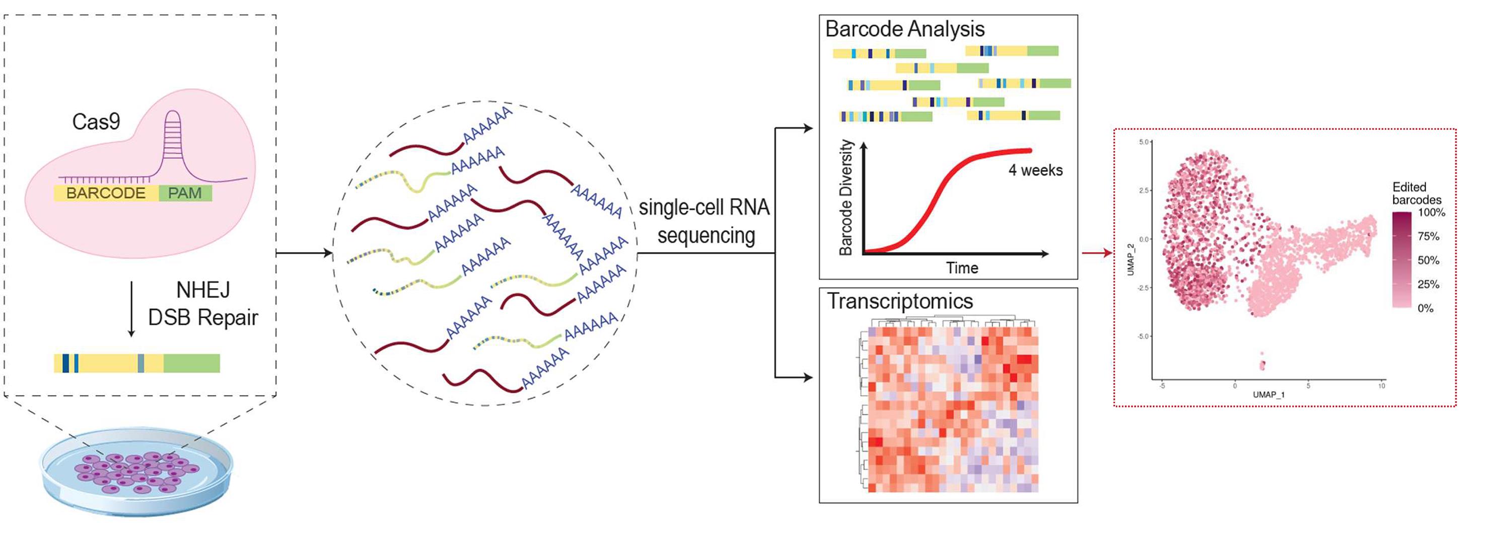
Graphical overview of the scDynaBar workflow
Background
Cellular behavior is inherently dynamic and changes in response to developmental programs and environmental signals. Capturing these time-resolved processes remains challenging because widely used approaches trade temporal resolution for scalability and molecular depth. Live-cell fluorescence microscopy can provide direct temporal measurements, but long-term imaging is constrained by phototoxicity/photobleaching and by practical limits in throughput and downstream analysis, particularly in complex or in vivo contexts [1,2]. In parallel, computational approaches that infer dynamics from single-cell RNA sequencing (scRNA-seq), such as RNA velocity and pseudotime methods, show limited temporal resolution [3,4].
DNA-based cellular “memory” systems have therefore emerged as powerful tools to record transient biological signals as permanent genomic changes that can be retrospectively decoded [5,6]. Many CRISPR-enabled recorders implement a “write” operation by inducing mutations or programmable edits at defined loci, thereby generating genetic barcodes that store information about cell history, lineage relationships, or stimulus exposure [5–7]. Importantly, CRISPR-based recording strategies can be coupled to sequencing-based readouts to integrate recorded information with single-cell profiling to jointly interrogate cellular state and history [8]. Together, these advances have led to a growing repertoire of molecular recording systems [6–15].
A specific goal within this space is to encode elapsed time through continuous or progressive mutagenesis [16,17]. Self-targeting guide RNA designs and related “DNA clock” strategies can generate mutations that accumulate over time, enabling retrospective estimation of event timing or duration [16,17]. However, this strategy is not readily compatible with standard 3′ scRNA-seq workflows, as the mutational barcodes are not polyadenylated, complicating joint analysis of transcriptomes and barcodes in the same cells and increasing experimental overhead [16]. As a result, there is a need for recording systems that (i) accumulate edits progressively over extended periods and (ii) are directly compatible with widely used scRNA-seq platforms.
This protocol describes the implementation of scDynaBar, a CRISPR-based recording strategy that supports long-term, tunable accumulation of mutational barcodes while remaining compatible with standard scRNA-seq capture [18]. In practical terms, the approach is designed to integrate into common single-cell workflows, enabling simultaneous profiling of transcriptomes and temporal barcodes at single-cell resolution. Compared with microscopy-based longitudinal tracking, this method is scalable and applicable to systems where imaging is impractical; compared with purely inference-based trajectory methods, it generates a physical record of prior activity encoded in DNA. Key limitations include not controlling the copy number, the need for efficient delivery of CRISPR components, calibration of editing rates to the cell type of interest, and accounting for locus- and context-dependent biases in editing outcomes [5,17]. Finally, the system can be adapted to record a wide range of stimuli or signals that can be coupled to Cas9 activity (e.g., via signal-responsive promoters) [7,15].
In the associated study, scDynaBar was implemented using both Cas9 nuclease-based editing and base-editing strategies [10], which both serve the same overall purpose of generating sequence-diversified barcodes that can be recovered by sequencing. Here, we focus on Cas9-based implementation of scDynaBar in mouse embryonic stem cells using both bulk amplicon sequencing and single-cell 10x Genomics 3′ RNA-seq, including barcode-enrichment libraries. We further describe the computational pipeline used to analyze data generated from both experimental setups. Example applications also include 3D gastruloids and a Zscan4-dependent Cas9 induction system, illustrating the use of scDynaBar to track the transition of mouse embryonic stem cells (mESCs) into the 2C-like state.
Materials and reagents
Biological materials
1. E14 mESC line
Reagents
Cell culture
1. DMEM high glucose, pyruvate (Gibco, catalog number: 11995040)
2. Fetal bovine serum (Gibco, catalog number: A5256701)
3. GlutaMax (Gibco, catalog number: 35050061)
4. Pen Strep (Gibco, catalog number: 15140122)
5. Non-essential aminoacids (Gibco, catalog number: 11140050)
6. β-mercaptoethanol (Gibco, catalog number: 31350010)
7. mLif (Stem Cell Institute, Cambridge)
8. DMEM/F12 (Thermo Fisher Scientific, catalog number: 11320033)
9. Neurobasal (Thermo Fisher Scientific, catalog number: 21103049)
10. N2 supplement (Cell Therapy Systems, catalog number: A1370701)
11. B-27 supplement (Thermo Fisher Scientific, catalog number: 17504044)
12. PBS (Thermo Fisher Scientific, catalog number: 14190144)
13. Trypsin-EDTA (Thermo Fisher Scientific, catalog number: 25200056)
14. Accutase (StemPro, catalog number: A1110501)
15. Trypan blue (0.4%) (Gibco, catalog number: 15250061)
16. Gelatin (Sigma, catalog number: G9391)
17. BSA (Gibco, catalog number: 15260037)
18. Fugene (Promega, catalog number: E2311)
19. Cre recombinase Gesicles (Takara, catalog number: 631449)
20. Polybrene (Sigma, catalog number: H9268)
21. 4-hydroxytamoxifen (Sigma, catalog number: H7904)
22. CHIR99021 (Department of Biochemistry, University of Cambridge)
23. Opti-MEMTM I reduced serum medium (Thermo Fisher Scientific, catalog number: 31985062)
RNA sequencing reagents
23. RNeasy Micro Kit (Qiagen, catalog number: 74004)
24. SuperScriptTM II, SuperScriptTM II first-strand buffer (5×) and DTT (100 mM) (Thermo Fisher Scientific, catalog number: 18064014)
25. Betaine (5 M) (Merck, catalog number: B0300)
26. MgCl2 (Promega, catalog number: A3511)
27. dNTPs (10 mM) (Thermo Fisher Scientific, catalog number: 18427013)
28. RNase inhibitor (Promega, catalog number: N2111)
29. KAPA HiFi HotStart ReadyMix (KAPA Biosystems, catalog number: KK2502)
30. AMPure XP beads (Beckman Coulter, catalog number: A63881)
31. 10× Single-Cell 3’ Library & Gel Bead kit v2 (10x Genomics, catalog number: PN120237)
32. Bulk sequencing primers:
a. Reverse transcription: GTGACTGGAGTTCAGACGTGTGCTCTTCCGATCTT(30)
b. First amplicon PCR:
Forward: 5′-ACACTCTTTCCCTACACGACGCTCTTCCGATCT(N/NN/NNN)TCTTGTGGAAAGGACGAAACAC-3′
Reverse: 5′-CAAGCAGAAGACGGCATACGAGATXXXXXXGTGACTGGAGTTCAGACGTGTGCTCTTCCGATCT-3′
c. Second amplicon PCR:
Forward: 5′-AATGATACGGCGACCACCGAGATCTACACTCTTTCCCTACACGACGCTCTTCCGATCT-3′
Reverse: 5′-CAAGCAGAAGACGGCATACGAGAT-3′
33. Single-cell sequencing primers:
a. First amplicon PCR:
Forward: 5′-ACACTCTTTCCCTACACGACGCTCTTCCGATCT(N/NN/NNN)TCTTGTGGAAAGGACGAAACAC-3′
Reverse: 5′-AATGATACGGCGACCACCGAGATCTACACTCTTTCCCTACACGACGCTCTTCCGATCT-3′
b. Second amplicon PCR:
Forward: 5′-CAAGCAGAAGACGGCATACGAGATXXXXXXXXGTGACTGGAGTTCAGACGTGTGCTCTTCCGATCT-3′
Reverse: 5′-AATGATACGGCGACCACCGAGATCTACACTCTTTCCCTACACGACGCTCTTCCGATCT-3′
Solutions
1. Base media for mESCs (see Recipes)
2. Gastruloid media (N2B27) (see Recipes)
Recipes
1. Base media for mESCs
| Component | Initial concentration | Volume (mL) | Final concentration |
|---|---|---|---|
| DMEM high glucose, pyruvate | 100% | 409.5 | 82% |
| Fetal bovine serum | 100% | 75 | 15% |
| GlutaMax | 200 mM | 5 | 2 mM |
| Pen Strep | 100× | 5 | 1× |
| Non-essential aminoacids | 100× | 5 | 1× |
| β-mercaptoethanol | 50 mM | 0.5 | 50 μM |
Add 50 μL of mLif to 50 mL of medium in a 50 mL Falcon to use as the working stock (to avoid repeated heating/cooling cycles of unused media). Use within a week.
2. Gastruloid media (N2B27)
| Component | Initial concentration | Volume (mL) | Final concentration |
|---|---|---|---|
| DMEM/F12 | 100% | 240.75 | 48% |
| Neurobasal | 100% | 240.75 | 48% |
| N2 supplement | 100× | 2.5 | 0.5× |
| B-27 supplement | 50× | 5 | 0.5× |
| GlutaMax | 200 mM | 5 | 2 mM |
| Pen Strep | 100× | 5 | 1× |
| β-mercaptoethanol | 50 mM | 1 | 0.1 mM |
Laboratory supplies
1. 6-well plate, tissue culture treated (Falcon, catalog number: 38016)
2. U-bottom 96-well suspension culture plate (Greiner Bio-One, catalog number: 650185)
3. Serological pipettes and pipette aid
4. Micropipettes, variable volume
5. Pipette tips, variable volume
6. 15 mL Falcon tubes
7. 50 mL Falcon tubes
8. 1.5 mL tubes
9. CountessTM cell counting chamber slides (Thermo Fisher, catalog number: C10228)
10. 50 μm strainer (Sysmex, catalog number: 1050553)
Equipment
1. Incubator with regulated temperature and humidity (37 °C, 5% CO2)
2. Centrifuges
3. Biological safety cabinet
4. 4 °C fridge, -20 °C freezer, and -80 °C freezer
5. Countess II automated cell counter (Thermo Fisher Scientific)
6. BD Aria III or BD Influx High-Speed Cell Sorter (BD Biosciences)
7. 10× Chromium device (10x Genomics, CAS 1000204)
Software and datasets
| Type | Software/dataset/resource | Version | Date | License | Access (free or paid) |
|---|---|---|---|---|---|
| Data | Raw sequencing data (FASTQ; scRNA-seq + single-cell barcode libraries + bulk barcodes) from the paper where this protocol is used [18] are deposited in NCBI GEO (accession: GSE280613 and GSE280614) | GEO terms | Free | ||
| Dataset/resource | Mouse reference genome mm10 (Cell Ranger reference) + GFP sequence (custom reference build) | Free | |||
| Software 1 | Cell Ranger (10x Genomics) | 10.0.0 | 10x Genomics | Free | |
| Software 2 | R | 4.3.2 | Free | ||
| Software 3 | Seurate (CRAN) | 5.4.0 | Free | ||
| Software 4 | ShortRead (Bioconductor) | 1.68.0 | Free | ||
| Software 5 | Biostrings (Bioconductor) | 2.78.0 | Free | ||
| Software 6 | data.table (CRAN) | 1.18.0 | Free | ||
| Code S1 | Bulk barcode extraction/QC: https://github.com/socyol/scDynaBar/blob/main/Bioprotocols/A_bulk_data_analysis/A1_fastq_to_csv.R | main branch | MIT License | Free | |
| Code S2 | Bulk metrics (uncuts/divergence): https://github.com/socyol/scDynaBar/blob/main/Bioprotocols/A_bulk_data_analysis/A2_metrics.R | main branch | MIT License | Free | |
| Code S3 | scRNA-seq processing in Seurat: https://github.com/socyol/scDynaBar/tree/main/Bioprotocols/B_singlecell-data_analysis | main branch | MIT License | Free | |
| Code S4 | Single-cell barcode processing + merge: https://github.com/socyol/scDynaBar/tree/main/Bioprotocols/B_singlecell-data_analysis | main branch | MIT License | Free |
1. R software (R version 4.3.2, 2023-10-31)
2. RStudio Desktop [Version 2023.03.1+446 (2023.03.1+446)]
3. Cell Ranger, free under 10x Genomics (Cell Ranger version 10.0.0, 2025-11-13)
4. Seurat R package (free) (Seurat version 5.4.0)
5. ShortRead Bioconductor package (free) (ShortRead version 1.68.0)
6. Biostrings Bioconductor package (free) (Biostrings version 2.78.0)
7. data.table R package (free) (data.table version 1.18.0)
8. All raw sequencing data have been deposited in GEO (accession numbers GSE280613 and GSE280614). All analysis scripts (bulk and single-cell) are available on GitHub (https://github.com/socyol/scDynaBar/tree/main/Bioprotocols).
Procedure
A. Vector construction
1. The barcoding vector was generated using an optimized piggyBac transposon backbone derived from the system described by Cadinanos and Bradley [19]. The construct consists of a CAG promoter driving mCherry expression, followed by a self-targeting single-guide RNA (sgRNA) expression cassette and a polyadenylation signal.
2. The complete sgRNA cassette sequence (U6 promoter–spacer–sgRNA scaffold) is shown in Figure 1. The spacer sequence used throughout this protocol was GGTATGCGGATGCAATCTCCG.
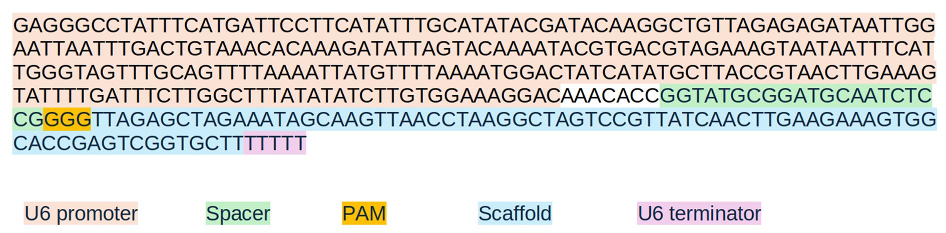
Figure 1. gRNA sequence used
3. The barcoding cassette was assembled by inserting two PCR-amplified synthetic DNA fragments (gBlocks; Integrated DNA Technologies, Coralville, IA, USA) into the piggyBac backbone by restriction enzyme cloning. The piggyBac backbone was digested with BbsI and XhoI, while the insert fragments were digested with BsaI/BamHI and BamHI/XhoI, respectively. Digested DNA fragments were purified using the Monarch PCR & DNA Cleanup kit and Monarch Gel Extraction kit (New England Biolabs) prior to ligation with T4 DNA ligase according to the manufacturer's instructions. Ligation products were transformed into chemically competent Escherichia coli DH5α cells and selected on LB agar plates containing ampicillin. Positive colonies were identified by colony PCR using primers flanking the sgRNA cassette, followed by plasmid purification and sequence verification.
4. The inducible Cas9 construct consists of a bicistronic Cas9-P2A-GFP [9] expression cassette under the control of the CAG promoter, cloned into the same optimized piggyBac backbone. Expression is regulated using a FLEX (Cre-On) switch in which alternating LoxP and Lox2272 sites maintain the coding sequence in an inactive orientation until Cre-mediated recombination irreversibly inverts the cassette into the transcriptionally active orientation, enabling temporal control of Cas9 expression [20]. A CMV-driven geneticin resistance cassette is included to allow selection of stable integrants.
5. For base-editing experiments, the BE3 editor described by Komor et al. [10] was modified by removing the uracil glycosylase inhibitor (UGI) domain to broaden the spectrum of editing outcomes. Whereas the UGI domain in the original BE3 editor promotes precise C:G-to-T:A substitutions, its removal increases the diversity of editing outcomes, including alternative substitutions and indels, thereby enhancing barcode diversity. The resulting nCas9-rAPOBEC1-P2A-GFP expression cassette was incorporated into the same piggyBac backbone under the control of the CAG promoter and the FLEX system. A CMV-driven geneticin resistance cassette was included to enable selection of stable integrants.
6. The pZscan4c-CreERT2 plasmid was generated by placing CreERT2 under the control of the Zscan4c promoter [21]. The vector also contains a CMV-driven puromycin resistance cassette to allow selection of stable transfectants.
7. All plasmids were verified by Sanger sequencing prior to experimental use.
Vector availability: The plasmids described in this protocol are available from the corresponding author upon request.
B. Mouse embryonic stem cell culture
1. Maintenance conditions: Culture E14 mESCs in mESCs basal media on gelatinized tissue-culture plates to support proper attachment. Maintain the cells at 37 °C in a humidified 5% CO2 atmosphere.
2. Feeding and passaging:
a. Exchange the medium daily using mESC basal media to maintain the pluripotent state.
b. Passage the cells every 48 h (every other day). For dissociation, use trypsin-EDTA.
3. Generation of stable clonal lines:
a. Perform cell transfection using Fugene reagent according to the manufacturer’s protocol.
i. Twenty-four hours prior to transfection, seed 300,000 cells in a well of a gelatin-coated six-well plate.
ii. Dilute 5 μg of plasmid DNA in Opti-MEMTM I Reduced Serum Medium and combine with Fugene HD at a 3:1 reagent-to-DNA ratio. The mixture includes the system’s vectors (the barcode cassette and the Cas9 construct) at a final concentration of 1.3 μg and Piggybac transposase at a final concentration of 1 μg.
iii. Incubate the mixture at room temperature for 15 min and then add drop-by-drop to the mESCs culture.
iv. Incubate cells for 24 h, after which a medium change is necessary for recovery for an additional 24 h.
b. Following transfection, apply drug selection (e.g., geneticin at 700 μg/mL for 3 days) and, once recovered, use fluorescence-activated cell sorting (FACS) of mCherry+ cells to enrich positive populations.
c. For single-cell clone expansion: Once the transfected cell populations have been obtained, perform single-cell sorting into gelatin-coated 96-well plates, ensuring that one cell is deposited per well. Culture the cells under appropriate growth conditions and monitor them regularly for colony formation. Allow 2–3 weeks for single cells to recover, proliferate, and expand into clonal colonies.
d. Visually inspect the surviving clones for mCherry fluorescence and select approximately 10 positive clones for genomic DNA extraction, PCR, and Sanger sequencing to confirm the integration of the Cas9 and the mCherry-barcode constructs. Most clones are expected to carry the integrated constructs.
4. Induction protocols:
a. Cas9 activation: Induce the barcoding system by adding Cre recombinase Gesicles to the media supplemented with 6 μg/mL polybrene, according to the manufacturer’s instructions. The efficiency of induction can be checked by FACS after 24–48 h.
b. 2C-like state transition: To track totipotency-like transitions, treat pZscan4c-CreERT2 cells with 1 μM 4-hydroxytamoxifen for 12 days.
C. Gastruloid culture
1. Induction of mESC clonal lines:
a. Maintain the mESC clonal cell line containing the barcoding system under standard serum/mLIF conditions.
b. Induce the barcoding system using Cre recombinase in media supplemented with 6 μg/mL polybrene, following the manufacturer’s instructions.
c. Incubate the cells for 48 h prior to the start of the gastruloid formation protocol.
2. Cell dissociation and gastruloid formation:
a. Dissociate the induced mESCs into a single-cell suspension using trypsin-EDTA.
b. Wash the cells twice with prewarmed PBS.
c. Resuspend the resulting cell pellet in 5 mL of N2B27 medium.
d. Dilute the cells to a final density of 7,500 cells/mL in N2B27 medium.
e. Add 40 μL of this cell suspension to each well of a U-bottom 96-well suspension culture plate to reach a final density of 300 cells per well.
f. Incubate the plates for 48 h at 37 °C to allow for cell aggregation.
3. Chemical induction and maintenance:
a. During the first 48 h, culture aggregates in the initial 40 μL of N2B27 medium.
b. At 48 h, add 150 μL of N2B27 supplemented with 3 μM CHIR99021 directly to each well without removing the original medium (final volume ~190 μL).
c. At 72, 96, and 120 h, carefully remove 150 μL of medium from the side of each well, leaving ~40 μL to avoid disturbing the gastruloid, and replace it with 150 μL of fresh prewarmed N2B27.
4. Harvesting and single-cell preparation:
a. Harvest the gastruloids on day 4.
b. Transfer the gastruloids to an Eppendorf tube, rinse once with PBS, and dissociate them into single cells using Accutase.
c. Wash the cells twice with 5 mL of PBS containing 0.04% BSA to effectively remove the dissociation reagent.
d. Pass the cell suspension through a 50 μm strainer to ensure a high-quality single-cell suspension.
e. Determine total cell count and viability using an automated cell counter (e.g., Countess II) before proceeding to single-cell sequencing.
D. Bulk barcode sequencing (amplicon library)
1. Cell sorting and collection:
a. Following stable integration and induction of the barcoding system, harvest the mixed, non-clonal cell population at the required time points.
b. Dissociate cells into a single-cell suspension and sort for double-positive (GFP+ and mCherry+) populations using a BD Aria III, BD Influx High-Speed Cell Sorter, or similar.
c. Collect at least 10,000 cells.
2. RNA extraction: Extract total RNA from the sorted cell pellets using the RNeasy Micro Kit according to the manufacturer’s instructions.
3. Reverse transcription (RT): Perform reverse transcription to amplify the gRNA loci using an optimized amount of total RNA (1 μg) as input and 1 μL of specific RT primer [5′-GTGACTGGAGTTCAGACGTGTGCTCTTCCGATCT-T(30)-3′] to target the polyadenylated expressed barcodes. Follow the cycling conditions of Table 1 in a final volume of 10 μL of reverse transcriptase mastermix [1× Superscript II first-strand buffer (5×), 2.5 mM DTT, 1 M Betaine, 9 mM MgCl2 (including 1× buffer), 1 mM dNTPs, 100 U SuperScript II (200 U/μL), 5 U RNase inhibitor, and RNase-free water to adjust the reaction volume].
Table 1. Reverse transcription cycling conditions
| Temperature (°C) | Time (min) |
|---|---|
| 42 | 60 |
| 50 | 30 |
| 60 | 10 |
4. Intermediate purification:
a. Allow AMPure XP beads to warm at room temperature for 15 min and vortex thoroughly to resuspend.
b. Spin the cDNA plate and add AMPure XP beads at a 0.8:1 volumetric ratio to each sample.
c. Mix well by pipetting up and down 10 times.
d. Incubate at room temperature for 5–10 min to allow DNA binding.
e. Place the tube on a magnetic stand for 2–5 min, until the beads are fully pelleted and the liquid is clear.
f. Carefully remove and discard the supernatant without disturbing the beads.
g. Keeping the tube on the magnet, wash the beads twice:
i. Add 200 μL of freshly prepared 80% ethanol: add the ethanol, pipette up and down, then eject. Change tips between washes.
ii. Repeat once more for a total of two washes.
h. Let the beads air-dry for 2–5 min. They should look glossy but not cracked (avoid over-drying).
i. Remove the tube from the magnet and resuspend the purified cDNA in a final volume of 12 μL.
5. First-round PCR:
a. Amplify the resulting cDNA in a 20 μL reaction using KAPA HiFi HotStart ReadyMix following the cycling conditions shown in Table 2.
b. Use the following primers to introduce sequence diversity and sample indices:
Forward: 5′-ACACTCTTTCCCTACACGACGCTCTTCCGATCT(N/NN/NNN)TCTTGTGGAAAGGACGAAACAC-3′
Reverse: 5′-CAAGCAGAAGACGGCATACGAGATXXXXXXGTGACTGGAGTTCAGACGTGTGCTCTTCCGATCT-3′ (where XXXXXX represents the unique sample index).
Index specification: The string XXXXXX represents a 6-base custom-designed sample index. These sequences are specific custom designs utilized for sample multiplexing.
Note: The random nucleotides (N, NN, or NNN) in the forward primer are critical to increase sequence diversity for high-quality cluster identification during Illumina sequencing.
Table 2. PCR1 cycling conditions
| Temperature (°C) | Time (min) | Number of cycles |
| 95 | 3 | 1 |
| 98 | 0:20 | 10* |
| 63 | 0:30 | |
| 72 | 0:30 | |
| 72 | 1 | 1 |
*The number of cycles must be optimized depending on the amount of RNA.
6. Intermediate purification:
a. Allow AMPure XP beads to warm at room temperature for 15 min and vortex thoroughly to resuspend.
b. Spin the cDNA plate and add AMPure XP beads at a 0.8:1 volumetric ratio to each sample.
c. Mix well by pipetting up and down 10 times.
d. Incubate at room temperature for 5–10 min to allow DNA binding.
e. Place the tube on a magnetic stand for 2–5 min, until the beads are fully pelleted and the liquid is clear.
f. Carefully remove and discard the supernatant without disturbing the beads.
g. Keeping the tube on the magnet, wash the beads twice:
i. Add 200 μL of freshly prepared 80% ethanol: add the ethanol, pipette up and down, then eject. Change tips between washes.
ii. Repeat once more for a total of two washes.
h. Let the beads air-dry for 2–5 min. They should look glossy but not cracked (avoid over-drying)
i. Remove the tube from the magnet and resuspend the purified DNA in a final volume of 20 μL.
7. Second-round PCR:
a. Perform a second PCR in a 20 μL reaction using KAPA HiFi ReadyMix to incorporate full-length Illumina adapters, following the cycling conditions shown in Table 3.
b. Use the following primers:
Forward: 5′-AATGATACGGCGACCACCGAGATCTACACTCTTTCCCTACACGACGCTCTTCCGATCT-3′
Reverse: 5′-CAAGCAGAAGACGGCATACGAGAT-3′.
Table 3. PCR2 cycling conditions
| Temperature (°C) | Time (min) | Number of cycles |
| 95 | 3 | 1 |
| 98 | 0:20 | 11 |
| 63 | 0:30 | |
| 72 | 0:30 | |
| 72 | 1 | 1 |
8. Final purification and sequencing:
a. Purify the final PCR products again with AMPure XP beads at a 0.8:1 ratio as before and resuspend in 12 μL of water.
b. Check the final product by Bioanalyzer to confirm a single sharp peak at 400–500, quantify, and pool libraries in equimolar amounts.
c. Sequence the library on an Illumina MiSeq platform using a single-end run with 58 cycles (producing a 58 bp amplicon) and an 8-cycle index read, spiking in a sufficient amount of PhiX control DNA (typically ≥20%) to increase base diversity for robust cluster identification.
E. Single-cell enrichment library
1. Cell loading and library preparation:
a. Load a single-cell suspension into the 10× Chromium device.
b. Prepare libraries using the 10x Genomics Single-Cell 3′ Library & Gel Bead Kit v2, following the manufacturer’s instructions.
c. Load each of the samples into a separate lane of the 10× Chromium Control chip.
2. First-round gRNA amplification (amplicon enrichment PCR):
a. Perform amplicon gRNA PCRs for each of the 10x Genomics cDNA samples using 1 μL of the cDNA and KAPA HiFi Readymix.
b. Use the following primers to amplify the barcode loci:
Forward: 5′-ACACTCTTTCCCTACACGACGCTCTTCCGATCT(N/NN/NNN)TCTTGTGGAAAGGACGAAACAC-3′.
Reverse: 5′-AATGATACGGCGACCACCGAGATCTACACTCTTTCCCTACACGACGCTCTTCCGATCT-3′.
Note: Random nucleotides (NNN, NN, and N) are added to the forward primer to introduce sequence diversity.
3. Purification and second-round nested PCR (indexing):
a. Purify the first-round PCR products using AMPure XP beads at a 0.8:1 volumetric ratio.
b. Resuspend the total volume and load it into a second nested PCR using KAPA HiFi Readymix to incorporate sample-specific indices.
c. Use the following indexing primers:
Forward: 5′-CAAGCAGAAGACGGCATACGAGATXXXXXXXXGTGACTGGAGTTCAGACGTGTGCTCTTCCGATCT-3′ (where XXXXXXXX represents the unique sample index).
Reverse: 5′-AATGATACGGCGACCACCGAGATCTACACTCTTTCCCTACACGACGCTCTTCCGATCT-3′.
Index specification: The string XXXXXXXX represents an 8-base custom-designed sample index. These are unique, custom-designed sequences incorporated during primer synthesis.
4. Final purification and sequencing:
a. Perform a final purification of the enriched gRNA libraries using AMPure XP beads at a 0.8:1 volumetric ratio.
b. Check product by Bioanalyzer to confirm the presence of the expected amplicon peak at 400–500 bp.
c. Pool the enriched gRNA libraries and sequence them alongside the corresponding transcriptome libraries on the Illumina NovaSeq platform.
Data analysis
A. Bulk barcode data processing (single-end)
This section describes the workflow used to process demultiplexed FASTQ files and quantify barcode editing in bulk samples using R (Figure 2). Bulk barcode amplicon sequencing is used as an initial calibration step to confirm that barcode editing accumulates over time before moving to single-cell experiments. This bulk analysis also provides an overview of the editing status of each sample, allowing barcode editing levels and barcode diversity to be compared across samples.
FASTQ files are first converted into CSV files to simplify downstream analysis. Each FASTQ read consists of four lines containing the read identifier, the nucleotide sequence, a separator, and the corresponding Phred quality scores. These elements are extracted and stored as separate columns (A1 section). The reads are then screened for the expected flanking regions surrounding the mutable barcode. Only reads containing both flanking regions are retained. Finally, the extracted barcode sequences are compared with the original unedited barcode sequence using pairwise alignment. This allows the detection of editing events within the barcode, including insertions, deletions, and substitutions. Then we can extract the following metrics:
• Coverage: Total number of barcode reads.
• Percentage of uncut barcodes (% Uncuts): Percentage of barcodes that match the original unedited reference barcode/spacer sequence. A high percentage of uncut barcodes indicates low editing activity, whereas a lower percentage indicates increased barcode modification.
• Length: Length, in nucleotides, of each extracted barcode sequence. Changes in barcode length reflect insertion and deletion events introduced during barcode editing.
• Divergence: Normalized measure of barcode modification relative to the original reference barcode/spacer sequence. Divergence is derived from the pairwise alignment score, where lower similarity to the reference sequence corresponds to higher divergence. Higher divergence values indicate greater accumulated editing within the barcode.
The resulting editing metrics are used to quantify barcode modification and diversity across bulk samples (A2 section).
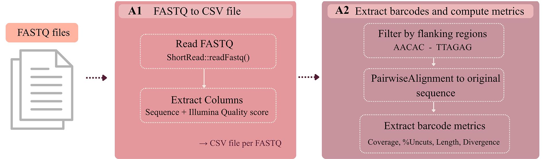
Figure 2. Bulk analysis workflow
All the code for this analysis has been uploaded on GitHub: A1_fastq_to_cvs.R for A1 analysis and A2_metrics.R script for A2.
Note: This pipeline was demonstrated using the publicly available dataset GSE280613; however, the same workflow can be applied to any demultiplexed bulk barcode FASTQ files generated with this library design. The full workflow is implemented in the following repository: socyol/scDynaBar (scripts: Bioprotocols/A_bulk_data_analysis/).
Input: Demultiplexed bulk FASTQ files (*.fastq.gz), one file per sample (Illumina MiSeq single-end), downloaded from GEO accession GSE280613 (example dataset).
Output:
1. Intermediate per-sample CSV files, containing read-level Sequence and Quality_sequence (Phred+33 ASCII) for each read.
2. Per-sample unique barcode tables saved as *_unique_barcode.csv, containing one row per unique barcode with count, Alignment_score, Uncuts, Length, and Divergence (min–max normalized within the sample).
3. Per-sample summary tables saved as *_summary.csv, containing coverage (sum of barcode counts), percent_uncut, and count-weighted mean metrics (e.g., mean Alignment_score and mean Divergence).
4. Combined summary table bulk_summary_all_samples.csv, containing one row per sample with coverage and count-weighted metrics across all processed samples.
A1. Convert FASTQ files to CSV
This section describes how to organize the demultiplexed barcode FASTQ files into a reproducible directory structure and the A1_fastq_to_csv.R script that (i) reads each FASTQ file, (ii) extracts the nucleotide sequence and per-base Phred quality string for every read, and (iii) saves one CSV file per sample for downstream barcode filtering and alignment.
1. Download the barcode FASTQ files.
2. Create a project folder and subfolder for the FASTQ files and output files.
mkdir -p scDynaBar_bulk/FASTQmkdir -p scDynaBar_bulk/Processed_CSVscd scDynaBar_bulk/FASTQ3. Open RStudio and install the required R packages:
## 1) Install CRAN package (data.table)install.packages("data.table")## 2) Install Bioconductor package (ShortRead)if (!requireNamespace("BiocManager", quietly = TRUE)) { install.packages("BiocManager")}BiocManager::install("ShortRead")BiocManager::install("Biostrings")4. Set the input and output directories at the beginning of the script.
fastq_dir <- "/ABS_PATH/scDynaBar_bulk/FASTQ_FOLDER"output_dir <- "/ABS_PATH/scDynaBar_bulk/Processed_CSVs"5. Extract the nucleotide sequence (Sequence) and the per-base Phred quality string (Quality_sequence) for each read by running the functions in the R script. It returns a data frame with one row per read. This function is applied to all FASTQ files.
Expected result: One CSV file per FASTQ is generated in Processed_CSVs/, containing Read, Sequence, Illumina Quality_sequence, and File (Figure 3).

Figure 3. Example output of 1_bulk_analysis.R. Each row corresponds to one sequencing read. The Quality_sequence field stores the raw Phred ASCII string for the full read; the barcode-region substring is extracted in Section A2 to compute QS_Illumina.
Note: This step stores the Phred quality string for each read; it is later used to compute mean Illumina Phred scores for the barcode region.
A2. Extract valid barcodes and compute per-read barcode metrics
This section is performed using the R script A2_metrics.R. The script processes the per-sample CSV files generated in Section A1 to (i) retain reads containing the constant flanking motifs (AACAC and TTAGAG), (ii) extract the barcode sequence located between the flanks, (iii) compute a barcode-level mean Illumina Phred quality score (QS_Illumina) and remove low-quality reads using the default threshold QS_Illumina < 28, (iv) collapse reads into unique barcodes with counts to reduce computation time, and (v) quantify barcode editing by global-local pairwise alignment of each unique barcode to a user-defined reference spacer sequence. The script outputs a per-sample barcode table and a per-sample summary file containing count-weighted editing metrics. The parameters used for the whole analysis are listed in Table 4.
Table 4. Default quality-control and alignment parameters used for scDynaBar barcode analysis
| Parameter | Default value | Description |
|---|---|---|
| flank1 | AACAC | 5′ constant motif (U6 promoter side); reads lacking this motif are discarded |
| flank2 | TTAGAG | 3′ constant motif (cassette side; reads lacking this motif are discarded) |
| spacer | 20 nt gRNA sequence | Reference sequence for pairwise alignment; must match the gRNA used in the sample |
| min_phred | 28 | Minimum mean Phred quality score over the barcode region; reads below this threshold are discarded |
| match | +2 | Substitution matrix score for a nucleotide match |
| mismatch | -1 | Substitution matrix score for a nucleotide mismatch |
| gap_open | 5 | Gap opening penalty for pairwise alignment |
| gap_ext | 5 | Gap extension penalty for pairwise alignment |
| Min_coverage (Bulk) | 200 | Minimum number of barcode reads per sample after filtering; samples below this threshold are excluded |
1. Choose one per-sample CSV file produced in Section A1 (e.g., Processed_CSVs/SAMPLE.csv).
2. Define the reference spacer sequence (21 nt) corresponding to the gRNA used in that sample (GGTATGCGGATGCAATCTCCG in our data).
3. Create an output folder to store barcode tables and summary files.
input_file <- "/ABS_PATH/scDynaBar_bulk/Processed_CSVs/SAMPLE.csv"output_dir <- "/ABS_PATH/scDynaBar_bulk/Barcodes_example/"spacer <- "GTATGCGGATGCAATCTCCG" # Example spacer; replace for other gRNAsdir.create(output_dir, showWarnings = FALSE, recursive = TRUE)4. Discard reads that do not contain both expected flanking motifs:
a. U6 promoter-side motif: AACAC.
b. Scaffold-side motif: TTAGAG.
d <- fread(input_file)sfl1 <- "AACAC"sfl2 <- "TTAGAG"d <- d[grepl(paste0(flank1, ".*", flank2), Sequence)]d <- d[!grepl("N", Sequence)]5. Compute the barcode metrics by running the R script 2_bulk_processing.R:
a. Percentage of original/uncut sequences by comparing extracted barcode/spacer sequences to the designed reference spacer sequence.
b. Length of the barcode.
c. Alignment of each barcode to the reference spacer using Biostrings pairwiseAlignment with a global-local strategy, scoring +2 (match) and –1 (mismatch), and gap opening and extension penalties = 5.
d. Divergence score as the mean alignment score across barcodes within each sample, and normalize divergence scores across all samples for comparability.
6. Exclude samples with fewer than 200 barcode reads remaining after filtering. This threshold may be adjusted depending on sequencing coverage.
Expected results:
1. SAMPLE_unique_barcodes.csv: One row per unique barcode, including count, Alignment_score, Divergence (min–max normalized within the sample), and additional barcode-level metrics (Figure 4).

Figure 4. Example output of SAMPLE_unique_barcodes.csv. Each row corresponds to one unique barcode detected after filtering. Barcode indicates the extracted barcode sequence; Counts indicates the number of reads supporting that barcode; Length indicates the barcode length in nucleotides; Alignment_score reports the pairwise alignment score against the reference barcode; Uncuts indicates whether the barcode matches the unedited original sequence; Insertions, Deletions, and Substitutions report the number of editing events detected; and Divergence represents the normalized divergence score from the reference barcode.
2. SAMPLE_summary.csv: A one-row per-sample summary including coverage (sum of counts), percent_uncut, and count-weighted mean metrics (e.g., mean Alignment_score and mean Divergence).
3. bulk_summary_all_samples.csv: One row per sample, containing coverage and count-weighted summary metrics for all processed samples (Figure 5).

Figure 5. Example output of bulk_summary_all_samples.csv. Each row corresponds to one processed bulk sample. File indicates the input sample file; Coverage indicates the total number of retained barcode reads after filtering; N_unique_barcodes indicates the number of distinct barcode sequences detected; Percent_Uncut represents the percentage of retained reads matching the unedited original barcode; Mean_length indicates the count-weighted mean barcode length in nucleotides; Mean_alignment_score reports the count-weighted mean pairwise alignment score against the reference barcode; and Mean_Divergence represents the count-weighted normalized divergence score.
B. Single-cell data analysis (scRNA-seq and barcode library integration)
This section describes the workflow used to process 10x Genomics scRNA-seq data and the paired-end scDynaBar barcode enrichment library and to integrate barcode-derived editing metrics with transcriptomic profiles at single-cell resolution (Figure 6). The scRNA-seq data are first processed with Cell Ranger (B1 section). The resulting filtered expression matrix is then analyzed in Seurat for quality control, normalization, clustering, and dimensionality reduction (B2 section).
In parallel, the barcode/amplicon FASTQ files are processed to recover a consensus barcode sequence for each cell ID–UMI pair. This involves extracting the 10x Genomics cell barcode and UMI from Read 1, extracting the editable barcode sequence from Read 2, applying quality and read-support filters, and selecting the most frequent barcode as the consensus sequence (B3 section). Consensus barcodes are then aligned to the reference spacer to compute barcode-level features and summarize them into per-cell metrics, including Coverage, Percentage of uncut barcodes, mean barcode length, and divergence (B4 section). These metrics are finally merged into the Seurat object as metadata, allowing barcode editing features to be visualized together with transcriptomic clusters and gene expression patterns (B5 section).
Note: Subsections B1–B4 provide working examples and reference scripts for reproducibility. We demonstrate the workflow using the publicly available dataset GSE280614; however, the same steps apply to any dataset generated with the same amplicon library structure. All scripts for this workflow are available in the GitHub repository socyol/scDynaBar, under Bioprotocols/B_singlecell-data_analysis/: B1_run_cellranger_count.sh, B2_analysis.R, B3_analysis_consensus_barcode.R, and B4_extract_barcode_features.R.
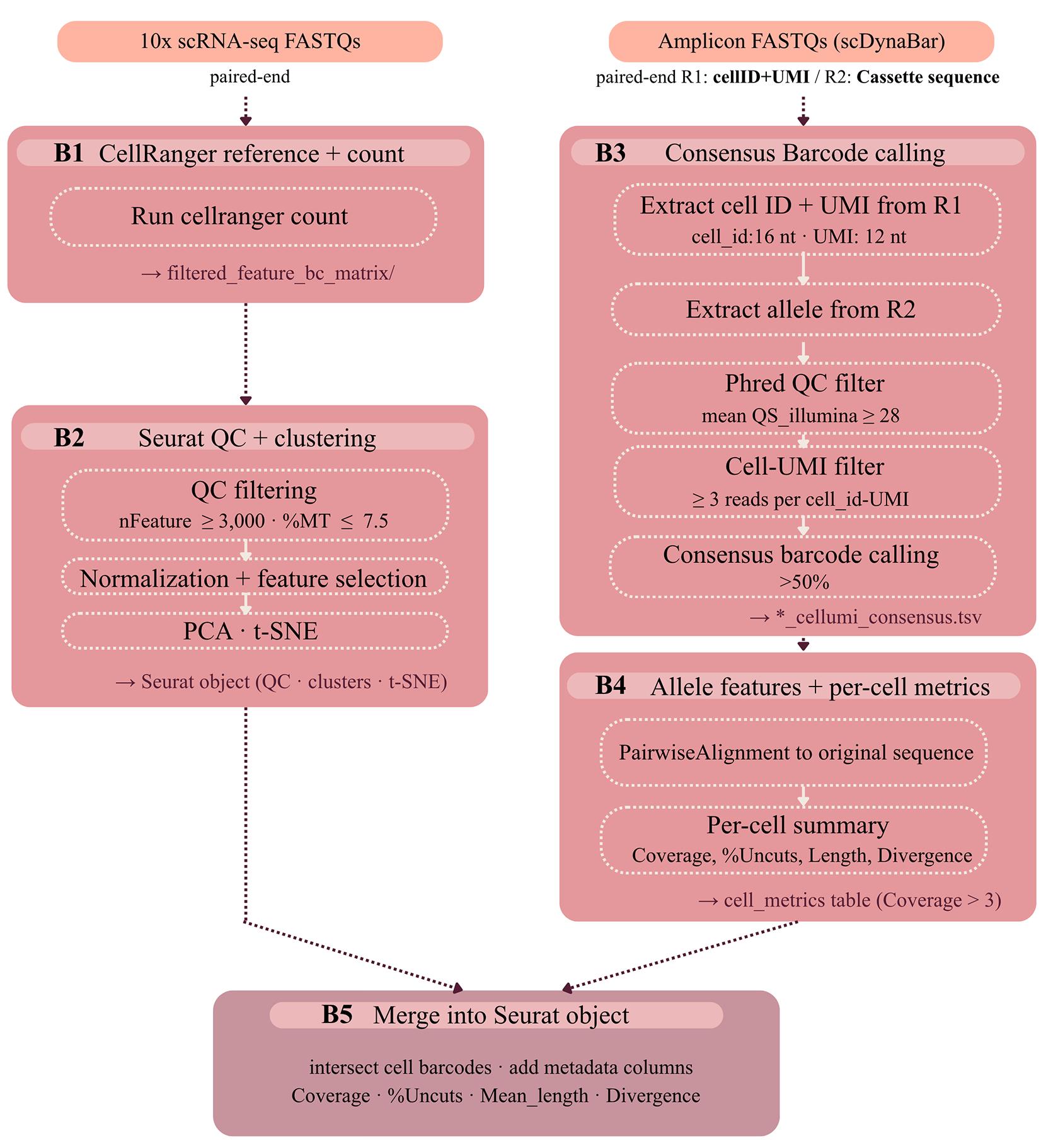
Figure 6. Single-cell analysis workflow
Input:
1. scRNA-seq FASTQs (paired-end) from 10x Genomics gene expression libraries.
2. Barcode/amplicon library FASTQs (paired-end), where R1 contains the 10x Genomics cell barcode + UMI, and R2 contains the scDynaBar amplicon/cassette.
Output:
1. A QC-filtered Seurat object containing normalized expression values, dimensionality reduction (PCA/t-SNE or UMAP), and clusters.
2. Per-cell barcode metrics table (e.g., Coverage, percent uncut, mean length, divergence).
3. Integrated Seurat object with barcode-derived metrics added as metadata, enabling joint visualization (e.g., t-SNE/UMAP colored by divergence or % uncut) and correlation with gene expression.
B1. Cell Ranger pipeline
Before running this step, download the paired-end scRNA-seq FASTQ files and place them in the corresponding FASTQ folder. This workflow was demonstrated using the publicly available dataset GSE280614, although the same procedure can be applied to any compatible 10x Genomics scRNA-seq dataset generated with the same library structure.
This step is performed using the Bash script: B1_run_cellranger_count.sh. This script performs the following steps:
1. Creates the project folder structure for scRNA-seq FASTQ files, Cell Ranger output files, and reference files.
2. Downloads and unpacks the prebuilt mouse Cell Ranger reference.
3. Runs cellranger count on the paired-end scRNA-seq FASTQ files.
4. Generates the filtered_feature_bc_matrix output used for downstream Seurat analysis.
Run the scripts from the terminal as follows:
chmod +x B1_run_cellranger_count.sh./B1_run_cellranger_count.shExpected result: Cell Ranger output files containing gene expression quantification for each single cell. The filtered_feature_bc_matrix output is used as input for the downstream Seurat analysis described in Section B2.
B2. Downstream scRNA-seq analysis (Seurat)
The downstream transcriptome analysis follows the Seurat-guided clustering workflow. For full details and updates, refer to the official Seurat tutorial. This step is performed using the Bash script: B2_scRNAseq_seurat.R, which performs the following steps:
1. Load the filtered matrix into Seurat (in RStudio).
2. For quality control filtering, discard cells with <3,000 detected genes and/or >7.5% mitochondrial UMIs.
so[["percent.mt"]] <- PercentageFeatureSet(so, pattern = "^mt-")so <- subset(so, subset = nFeature_RNA >= 3000 & percent.mt <= 7.5)3. Normalization and feature selection.
so <- NormalizeData(so)so <- FindVariableFeatures(so)so <- ScaleData(so)4. Dimensionality reduction and clustering
a. Perform broad clustering and visualization in Seurat.
b. Identify highly variable genes (e.g., FindVariableGenes) and run PCA (e.g., RunPCA) using these genes as input.
c. Use the first 15 principal components to compute clusters (Louvain; e.g., FindClusters) and generate t-SNE embeddings/plots.
Expected result: A Seurat object containing QC-filtered cells, normalized expression values, PCA embeddings, clusters, and a t-SNE representation.
B3. Consensus barcode calling from paired-end amplicon FASTQs
This section describes the processing of paired-end FASTQ files generated from the targeted scDynaBar barcode/amplicon library to recover a high-confidence consensus barcode sequence for each cell ID–UMI pair. In this library, Read 1 (R1) contains the 10x Genomics cell barcode followed by the UMI, whereas Read 2 (R2) contains the amplified scDynaBar cassette (Figure 7).
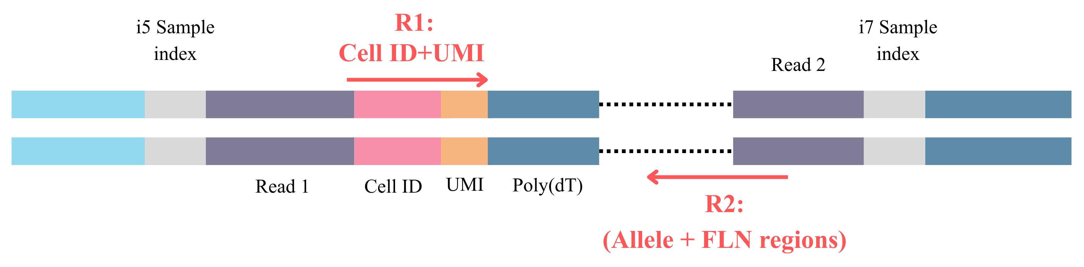
Figure 7. Read structure used for the single-cell barcode (amplicon) library. Read 1 (R1) contains the 10x Genomics cell barcode (first 16 nt) followed by the UMI (next 12 nt). Read 2 (R2) contains the scDynaBar amplicon sequence from which the barcode is extracted between constant flanking motifs. Schematic adapted from the 10x Genomics library read structure.
The analysis is performed using the R script B3_analysis_consensus_barcode.R. The script performs the following steps:
1. Loads required packages and sets input paths.
2. Loads the paired-end amplicon FASTQ files.
3. Extracts the cell ID and UMI from R1.
4. Extracts the barcode sequence from R2 using the constant flanking motifs surrounding the editable spacer.
5. Calculates the mean Phred quality score for the extracted barcode region.
6. Removes reads without the expected flanking motifs or with a mean barcode Phred score below 28.
7. Retains only cell ID–UMI groups supported by at least three reads.
8. Counts all barcode candidates observed for each cell ID–UMI pair.
9. Calls a consensus barcode by selecting the most frequent.
10. Flags consensus calls as passing when the top barcode represents more than 50% of the reads assigned to that cell ID–UMI pair.
11. Saves read-level, barcode-count, and consensus-level output tables.
Before running the script, modify the input paths, sample name, output directory, and flanking sequences according to the experimental design. In the example provided here, the expected read structure is a 16-nt cell barcode followed by a 12-nt UMI in R1, and the barcode is extracted from R2 between the selected constant flanking motifs.
Expected results:
1. SAMPLE_filtered_reads.tsv: Read-level table containing reads that pass flank filtering, mean Phred ≥28, and the cell_id–UMI support threshold (≥3 reads).
2. SAMPLE_cellumi_barcode_counts.tsv: Counts per cell_id–UMI–barcode (number of reads supporting each barcode candidate).
3. SAMPLE_cellumi_consensus.tsv: One consensus barcode per cell_id–UMI, with consensus_pass (= TRUE when the top barcode represents >50% of retained reads) (Figure 8).

Figure 8. Example output of SAMPLE_cellumi_consensus.tsv. Each row corresponds to one unique cell ID–UMI pair after consensus barcode calling. Cell_ID indicates the 10x Genomics cell barcode; UMI indicates the unique molecular identifier; cell_umi combines both identifiers; consensus_barcode indicates the barcode sequence selected as the consensus for that cell ID–UMI pair; Total_reads indicates the total number of reads assigned to that cell ID–UMI; Top_reads indicates the number of reads supporting the most frequent barcode; Top_fraction represents the fraction of reads supporting the consensus barcode; N_diff_barcodes indicates the number of different barcode sequences detected for that cell ID–UMI; and Consensus_pass indicates whether the consensus call passed the required threshold.
B4. Extract barcode features and compute per-cell metrics
This section describes how to compute barcode-level features from the consensus barcode table (*_cellumi_consensus.tsv) and summarize these features at the cell level. We quantify barcode editing by aligning each consensus barcode to the designed reference spacer using Biostrings::pairwiseAlignment() (global-local alignment; match = +2, mismatch = -1; gap opening = 5; gap extension = 5). We then compute per-cell summary metrics, including coverage, percent uncut, mean length, and a divergence score derived from alignment scores and normalized for comparability across cells.
Note: The complete implementation is provided in the script B4_extract_barcode_features.R. Below, we provide a minimal working example for clarity.
1. Load required packages and the consensus table produced in Section B3.
library(Biostrings)library(data.table)cons <- fread("/ABS_PATH/SAMPLE_cellumi_consensus.tsv")cons <- cons[consensus_pass == TRUE]2. Define the reference spacer sequence corresponding to the gRNA used in the experiment (example shown):
spacer <- DNAString("GGTATGCGGATGCAATCTCCGGGG")sigma <- nucleotideSubstitutionMatrix(match = 2, mismatch = -1, baseOnly = TRUE)3. Align each consensus barcode to the reference spacer and compute barcode features:
align_one <- function(barcode_seq) { aln <- pairwiseAlignment( spacer, DNAStringSet(barcode_seq), type = "global-local", substitutionMatrix = sigma, gapOpening = 5, gapExtension = 5 ) data.table( Alignment_score = aln@score, Length = nchar(barcode_seq), Uncuts = ifelse(as.character(aln@subject) == as.character(spacer), "YES", "NO") )}feat <- rbindlist(lapply(cons$consensus_barcode, align_one))barcode_table <- cbind(cons[, .(Cell_ID = cell_id, UMI = umi, barcode = consensus_barcode, total_reads)], feat)4. Compute a divergence score from alignment scores. Define divergence as the negative alignment score and min–max normalize to 0–1 across the dataset being summarized (e.g., within one sample):
barcode_table [, DIVERGENCE := -Alignment_score]barcode_table [, DIVERGENCE := (DIVERGENCE - min(DIVERGENCE)) / (max(DIVERGENCE) - min(DIVERGENCE))]5. Summarize barcode metrics per cell.
cell_metrics <- barcode_table [, .( Coverage = .N, # number of cell_id–UMI entries (or barcodes) retained Mean_length = mean(Length, na.rm = TRUE), DIVERGENCE = mean(DIVERGENCE, na.rm = TRUE), Uncuts = 100 * mean(Uncuts == "YES", na.rm = TRUE)), by = Cell_ID]# require minimal coverage per cellcell_metrics <- cell_metrics[Coverage > 3]Expected results:
1. SAMPLE_barcode_table.tsv: A table containing one row per retained Cell_ID–UMI consensus barcode. For each barcode, the table reports the cell ID, UMI, consensus barcode sequence, number of supporting reads, alignment score against the reference spacer, length, uncut status, and normalized divergence score (Figure 9).

Figure 9. Example output of SAMPLE_barcode_table.tsv. Each row corresponds to one retained Cell_ID–UMI consensus barcode after alignment to the reference barcode sequence. Cell_ID indicates the 10x Genomics cell barcode; UMI indicates the unique molecular identifier; Barcode indicates the consensus barcode sequence; Coverage reports the number of reads supporting that consensus barcode; Uncuts indicates whether the barcode matches the unedited original sequence; Length indicates the barcode length in nucleotides; Alignment_score reports the pairwise alignment score against the reference barcode; Divergence_raw represents the difference between the maximum reference alignment score and the observed alignment score; and Divergence represents the normalized divergence score relative to the best and worst alignment scores considered in the analysis.
2. SAMPLE_cell_metrics.tsv summarizes barcode-derived metrics at the cell level. Each row corresponds to one cell and includes the number of retained Cell_ID–UMI entries, mean barcode length, mean divergence, and percentage of uncut barcode inside the cell (Figure 10). After filtering cells by minimum barcode coverage, these metrics are merged into the Seurat object as metadata. The resulting object can be used for downstream visualization of barcode editing features on t-SNE or UMAP embeddings.
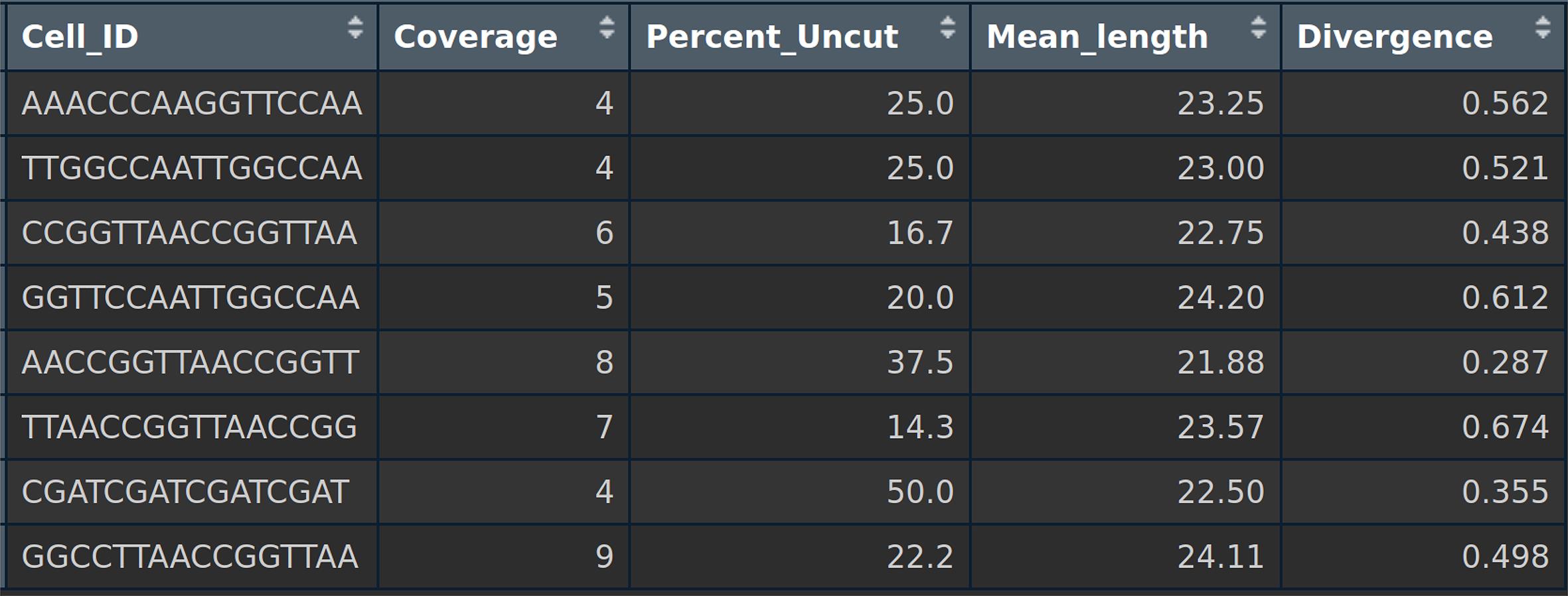
Figure 10. Example output of SAMPLE_cell_metrics.tsv. Each row corresponds to one cell after summarizing the retained Cell_ID–UMI consensus barcodes. Cell_ID indicates the 10x Genomics cell barcode; Coverage indicates the number of retained consensus barcodes assigned to that cell; Percent_Uncut represents the percentage of retained barcodes classified as uncut within that cell; Mean_length represents the mean barcode length in nucleotides; and Divergence indicates the mean normalized divergence score relative to the reference barcode.
B5. Merge barcode metrics with the Seurat object
This section describes how to integrate per-cell barcode metrics (Section B3) with the corresponding scRNA-seq Seurat object (Section B2). This enables joint analyses linking transcriptional state (gene expression) with barcode-derived temporal/editing metrics.
1. Load the Seurat object generated after scRNA-seq QC and clustering (Section G):
so <- readRDS("/ABS_PATH/SEURAT_OBJECT.rds")2. Identify cells present in both datasets and subset the Seurat object:
common_cells <- intersect(colnames(so), cell_metrics$Cell_ID)so <- so[, common_cells]3. Merge barcode metrics into Seurat metadata:
so@meta.data$Cell_ID <- rownames(so@meta.data)so@meta.data <- merge(so@meta.data, cell_metrics, by = "Cell_ID", all.x = TRUE)# restore rownames after mergerownames(so@meta.data) <- so@meta.data$Cell_IDExpected result: The Seurat object contains additional metadata columns (e.g., Coverage, Divergence, Mean_length, %Uncuts) and can be used to visualize barcode metrics on UMAP/t-SNE or correlate them with gene expression.
Note: If your Seurat object uses a different cell barcode format (e.g., suffixes like -1), ensure the Cell_ID strings match exactly between tables before merging.
Timing
1. Stable cell-line generation: approximately 3–4 weeks.
a. Transfection and selection: ~1 week.
b. Single-cell sorting and recovery: 2–3 weeks, depending on the growth characteristics of the cell line.
2. Gastruloid generation: 6 days.
3. RNA extraction and library preparation:
a. Bulk libraries: RNA extraction time can vary depending on the total number of samples. However, once RNA is extracted, samples can be processed in 96-well plates. The downstream library preparation workflow, including reverse transcription and PCR amplification steps, typically requires 1 day.
b. Single-cell libraries: Approximately 1 day is required for the specific amplification and enrichment of the genetic barcode libraries from the 10x Genomics cDNA.
4. Sequencing: 1 day. Sequencing time may vary depending on the sequencing platform, run configuration, and instrument availability.
5. Computational analysis: Once familiar with the code, the estimated analysis time is approximately 1–2 days. This includes preprocessing of sequencing data, barcode extraction, quality filtering, computation of barcode editing metrics, and integration of barcode information with single-cell transcriptomic data.
Result interpretation
The barcode-derived metrics obtained with this workflow provide a compact readout of cumulative scDynaBar editing activity at single-cell resolution.
The percentage of uncut sequences reflects the proportion of barcodes that remain unedited. Higher values indicate little or no editing, whereas lower values indicate progressive accumulation of edits over time. In the single-cell time-course experiment of [18], the percentage of uncut sequence decreases from day 0 to day 10, consistent with progressive barcode editing (Figure 11, left panel).
Divergence measures how different each barcode is from the original reference spacer based on pairwise alignment. Higher divergence values indicate greater deviation from the original sequence and therefore a longer or stronger history of editing. In the single-cell time-course experiment, divergence increases over time and also becomes more variable across cells, reflecting heterogeneous editing dynamics among individual cells (Figure 11, right panel).
Mean barcode length captures structural changes in the barcode sequence caused by insertions and deletions. Increased variation in barcode length is consistent with progressive editing and can provide additional information complementary to divergence and percent uncut sequence.
Together, these metrics allow the user to distinguish recently edited cells from cells with a longer barcoding history and to integrate this information with transcriptomic cell states.
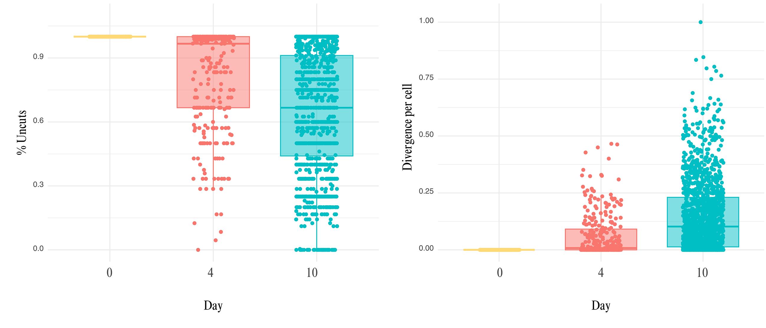
Figure 11. Single-cell time-course analysis from the scDynaBar paper [18] showing barcode divergence per cell (right) and percentage of uncut sequence (left) across days 0, 4, and 10
Validation of protocol
This protocol has been used and validated in the following research article: Andres-Lopez et al. [18]. It demonstrates that the dynamic barcoding system is highly reproducible, showing a Pearson’s correlation of 0.94 between biological replicates. In single-cell applications using the 10x Genomics platform, a barcode recovery efficiency of 97%–98% among cells that passed transcriptomic quality control was achieved.
The protocol was also applied to 3D mouse gastruloids to assess barcode recovery and editing across different cell types at day 6. After transcriptomic and barcode quality control, Cas9-GFP-positive cells were mapped to a mouse embryo reference atlas to assign cell-type identities. The annotated gastruloids showed a bias toward mesodermal lineages, consistent with previous studies showing that gastruloids often favor mesodermal or ectodermal cell types [22]. The fraction of original barcode sequences (median value 0.85) and barcode divergence values (median value 0.04) were broadly consistent across annotated cell populations, with no significant differences in barcoding rate across cell types (Kruskal–Wallis test, P = 0.3557; Kruskal–Wallis test, P = 0.319). These results support the application of scDynaBar to mESC-derived 3D gastruloids.
Application of the protocol
To demonstrate that the system can record dynamic state transitions, the protocol was applied to track entry into the 2C-like state in mESCs using a pZscan4-CreERT2 reporter strategy: upon tamoxifen treatment, cells entering the 2C-like state permanently activated the barcoding cassette and were profiled by paired scRNA-seq and barcode sequencing. Cells expressing Zscan4c (2C-like) consistently displayed low barcode divergence and a high fraction of uncut barcode sequences, consistent with recent activation of the barcoding cassette, indicating they had only recently transitioned into that state, whereas pluripotent cells showed greater variability in divergence scores.
General notes and troubleshooting
General notes
1. Implementation of baseline controls: To quantify background noise and ensure observed mutations result from active CRISPR targeting, the following controls are recommended:
• Uninduced baseline (day 0): Analyze cells prior to induction (e.g., before adding Cre or tamoxifen) to establish a baseline for background editing.
• Control without Cas9: Sequence cells transfected solely with the barcoding cassette (omitting Cas9/BE3 expression vectors) to identify spontaneous mutations or errors introduced during library preparation and sequencing.
• Late uninduced control: Collect and sequence non-induced cells at a later experimental time point (e.g., day 30) to evaluate the "leakiness" or spontaneous activation of the system over time.
2. Genomic integration and copy number control: Although the use of the piggyBac transposon system generally results in a low number of genomic insertions, the exact number of copies integrated into the genome cannot be controlled.
a. Expression monitoring: Beyond verifying the presence of the construct, the transcriptional expression levels of the barcoding and editing components (Cas9 or BE3) can be measured by RT-qPCR to confirm robust transcriptional activation following induction.
3. Biological models: The scDynaBar system was tested in two biological models:
a. 2C-like state transitions in mESCs: This illustrates how barcode diversity can function as a molecular clock to resolve the timing of a transient cellular event. Using a Zscan4c-driven CreERT2, barcode editing was coupled to the transition from pluripotency to a totipotent-like state, proving that these cells are transient and had only recently entered that state. The molecular clock revealed that the 2C-like population consisted exclusively of cells with low barcode diversity, meaning they had only recently transitioned into that state and had not yet had time to accumulate significant genetic mutations.
b. Mouse gastruloids: This 3D model demonstrates the applicability of scDynabar across other cell types. It shows that barcode editing rate remains consistent across different cell types and that active barcoding does not compromise cell differentiation.
4. Requirements for application in other biological systems: To implement scDynaBar in a different system, the following core requirements must be met:
a. Stable integration: The system requires the stable integration of the scDynaBar cassette (e.g., via piggyBac or lentiviral vectors) into the target cell line to ensure accurate record-keeping across cell divisions.
b. Inducible activation: A regulated induction system, such as the Cre-responsive FLEX switch used here, is essential for providing precise temporal or lineage-specific control over when the molecular clock begins to run.
Code availability: All analysis scripts and example commands are available at GitHub.
Troubleshooting
1. Transfection: Transfection efficiency is cell type specific. Optimize the transfection method for the target cells—for example, Lipofectamine or Lipostem for hiPSCs, or electroporation for difficult-to-transfect cell types.
2. Antibiotic selection: Antibiotic concentrations must be determined for each cell type by performing a kill curve. Some cell types can be very sensitive to certain antibiotics and resistant to others, so the resistance gene can be exchanged depending on the specific cell line used.
3. Single-cell sorting for clonal selection: Some cell types (e.g., hiPSCs) are too sensitive for single-cell sorting due to poor survival following single-cell dissociation. For these cells, manual colony picking is the preferred method for generating stable clonal cell lines.
4. Induction: Induction efficiency with exogenous Cre can be highly variable and is dependent on the initial cell seeding conditions. A doxycycline-inducible Cas9 system may offer more consistent and reproducible results.
5. Library preparation: Optimize the RNA input and number of PCR cycles according to the cell type and RNA quantity. For low-input RNA samples, we recommend using 300 ng of total RNA and resuspend the purified cDNA in a small volume to allow the entire cDNA yield to be used for the first PCR.
6. Amplicon overamplification: If the Bioanalyzer profile shows additional unexpected peaks indicative of overamplification, reduce the number of PCR cycles and/or increase the DNA input to improve library quality.
7. Poor sequencing quality or cluster identification failure: Low sequence diversity caused by identical constant regions in barcode libraries can impair cluster identification. Use primers with random nucleotides (N, NN, or NNN) and include ≥20% PhiX control DNA to increase base diversity and improve sequencing quality.
8. Calibration of editing rates: Before applying scDynaBar in a new experimental system or cell type, we recommend performing a pilot bulk amplicon sequencing time-course to characterize editing kinetics. This preliminary experiment enables the identification of time points during which the system is still actively editing, ensuring that barcode diversity continues to accumulate.
Acknowledgments
I.H.-H. was supported by a Ramón y Cajal Fellowship (RYC2020-028998-I), funded by MICIU/AEI/10.13039/501100011033 and the European Social Fund (FSE). C.E.K.-G. was supported by an FI-STEP AGAUR fellowship (2025-00376). This project was funded by MICIU/AEI/10.13039/501100011033 and the European Social Fund (FSE) (grants PID2022-137540NA-I00, EUR2025-165067, and CNS2023-144846), and by the European Union (ERC, DECODEM, Grant Agreement No. 101222344).
This protocol was used in [18].
Author contributions
Conceptualization, I.H.-H.; Investigation, C.E.K.-G., Y.A.-L., I.H.-H.; Writing—Original Draft, C.E.K.-G., Y.A.-L.; Writing—Review & Editing, C.E.K.-G., Y.A.-L., I.H.-H.; Funding acquisition, C.E.K.-G., I.H.-H.; Supervision, I.H.-H.
Competing interests
The authors declare no conflict of interest.
References
- Lac, A., Le Lam, A. and Heit, B. (2022). Optimizing Long-Term Live Cell Imaging. Methods Mol Biol. 2440: 57–73. https://doi.org/10.1007/978-1-0716-2051-9_3
- Maška, M., Ulman, V., Delgado-Rodriguez, P., Gómez-de-Mariscal, E., Nečasová, T., Guerrero Peña, F. A., Ren, T. I., Meyerowitz, E. M., Scherr, T., Löffler, K., et al. (2023). The Cell Tracking Challenge: 10 years of objective benchmarking. Nat Methods. 20(7): 1010–1020. https://doi.org/10.1038/s41592-023-01879-y
- La Manno, G., Soldatov, R., Zeisel, A., Braun, E., Hochgerner, H., Petukhov, V., Lidschreiber, K., Kastriti, M. E., Lönnerberg, P., Furlan, A., et al. (2018). RNA velocity of single cells. Nature. 560(7719): 494–498. https://doi.org/10.1038/s41586-018-0414-6
- Haghverdi, L., Büttner, M., Wolf, F. A., Buettner, F. and Theis, F. J. (2016). Diffusion pseudotime robustly reconstructs lineage branching. Nat Methods. 13(10): 845–848. https://doi.org/10.1038/nmeth.3971
- Sheth, R. U. and Wang, H. H. (2018). DNA-based memory devices for recording cellular events. Nat Rev Genet. 19(11): 718–732. https://doi.org/10.1038/s41576-018-0052-8
- Farzadfard, F. and Lu, T. K. (2018). Emerging applications for DNA writers and molecular recorders. Science. 361(6405): 870–875. https://doi.org/10.1126/science.aat9249
- Sheth, R. U., Yim, S. S., Wu, F. L. and Wang, H. H. (2017). Multiplex recording of cellular events over time on CRISPR biological tape. Science. 358(6369): 1457–1461. https://doi.org/10.1126/science.aao0958
- Wagner, D. E. and Klein, A. M. (2020). Lineage tracing meets single-cell omics: opportunities and challenges. Nat Rev Genet. 21(7): 410–427. https://doi.org/10.1038/s41576-020-0223-2
- Cong, L., Ran, F. A., Cox, D., Lin, S., Barretto, R., Habib, N., Hsu, P. D., Wu, X., Jiang, W., Marraffini, L. A., et al. (2013). Multiplex Genome Engineering Using CRISPR/Cas Systems. Science. 339(6121): 819–823. https://doi.org/10.1126/science.1231143
- Komor, A. C., Kim, Y. B., Packer, M. S., Zuris, J. A. and Liu, D. R. (2016). Programmable editing of a target base in genomic DNA without double-stranded DNA cleavage. Nature. 533(7603): 420–424. https://doi.org/10.1038/nature17946
- Anzalone, A. V., Randolph, P. B., Davis, J. R., Sousa, A. A., Koblan, L. W., Levy, J. M., Chen, P. J., Wilson, C., Newby, G. A., Raguram, A., et al. (2019). Search-and-replace genome editing without double-strand breaks or donor DNA. Nature. 576(7785): 149–157. https://doi.org/10.1038/s41586-019-1711-4
- Tang, W. and Liu, D. R. (2018). Rewritable multi-event analog recording in bacterial and mammalian cells. Science. 360(6385): eaap8992. https://doi.org/10.1126/science.aap8992
- Farzadfard, F., Gharaei, N., Higashikuni, Y., Jung, G., Cao, J. and Lu, T. K. (2019). Single-Nucleotide-Resolution Computing and Memory in Living Cells. Mol Cell. 75(4): 769–780.e4. https://doi.org/10.1016/j.molcel.2019.07.011
- Choi, J., Chen, W., Minkina, A., Chardon, F. M., Suiter, C. C., Regalado, S. G., Domcke, S., Hamazaki, N., Lee, C., Martin, B., et al. (2022). A time-resolved, multi-symbol molecular recorder via sequential genome editing. Nature. 608(7921): 98–107. https://doi.org/10.1038/s41586-022-04922-8
- Chen, W., Choi, J., Li, X., Nathans, J. F., Martin, B., Yang, W., Hamazaki, N., Qiu, C., Lalanne, J. B., Regalado, S., et al. (2024). Symbolic recording of signalling and cis-regulatory element activity to DNA. Nature. 632(8027): 1073–1081. https://doi.org/10.1038/s41586-024-07706-4
- Perli, S. D., Cui, C. H. and Lu, T. K. (2016). Continuous genetic recording with self-targeting CRISPR-Cas in human cells. Science. 353(6304): eaag0511. https://doi.org/10.1126/science.aag0511
- Park, J., Lim, J. M., Jung, I., Heo, S. J., Park, J., Chang, Y., Kim, H. K., Jung, D., Yu, J. H., Min, S., et al. (2021). Recording of elapsed time and temporal information about biological events using Cas9. Cell. 184(4): 1047–1063.e23. https://doi.org/10.1016/j.cell.2021.01.014
- Andres-Lopez, Y., Santambrogio, A., Kafetzopoulos, I., Todd, C. D., El Khouri-Gonzalez, C., Gonzalez-Alvarez, J. E., Alda-Catalinas, C., Clark, S. J., Reik, W., Hernando-Herraez, I., et al. (2026). Using CRISPR barcoding as a molecular clock to capture dynamic processes at single-cell resolution. Genome Res. 36(5): 1005–1015. https://doi.org/10.1101/gr.280915.125
- Cadinanos, J. and Bradley, A. (2007) Generation of an inducible and optimized piggyBac transposon system. Nucleic Acids Res 35: e87–e87. pmid:17576687
- Atasoy, D., Aponte, Y., Su, H. H. and Sternson, S. M. (2008). A FLEX Switch Targets Channelrhodopsin-2 to Multiple Cell Types for Imaging and Long-Range Circuit Mapping. J Neurosci. 28(28): 7025–7030. https://doi.org/10.1523/jneurosci.1954-08.2008
- Zalzman, M., Falco, G., Sharova, L. V., Nishiyama, A., Thomas, M., Lee, S. L., Stagg, C. A., Hoang, H. G., Yang, H. T., Indig, F. E., et al. (2010). Zscan4 regulates telomere elongation and genomic stability in ES cells. Nature. 464(7290): 858–863. https://doi.org/10.1038/nature08882
- Rosen, L. U., Stapel, L. C., Argelaguet, R., Barker, C. G., Yang, A., Reik, W. and Marioni, J. C. (2022). Inter-gastruloid heterogeneity revealed by single cell transcriptomics time course: implications for organoid based perturbation studies. bioRxiv: e509783. https://doi.org/10.1101/2022.09.27.509783
Article Information
Publication history
Received: May 25, 2026
Accepted: Jul 14, 2026
Available online: Jul 30, 2026
Published: Sep 5, 2026
Copyright
© 2026 The Author(s); This is an open access article under the CC BY-NC license (https://creativecommons.org/licenses/by-nc/4.0/).
How to cite
Andres-Lopez, Y., El Khouri-Gonzalez, C. and Hernando-Herraez, I. (2026). scDynaBar: A Step-By-Step Experimental and Computational Guide for Time-Resolved CRISPR Barcoding at Single-Cell Resolution. Bio-protocol 16(17): e5793. DOI: 10.21769/BioProtoc.5793.

 Download Citation in RIS Format
Category
Bioinformatics and Computational Biology
Biological Sciences > Biological techniques > CRISPR/Cas9
Cell Biology > Cell engineering > Barcoding
Do you have any questions about this protocol?
Post your question to gather feedback from the community. We will also invite the authors of this article to respond.
 Post a Question


