


- Protocols

- Articles and Issues
- For Authors
- About
- Become a Reviewer


Actin Quantification Using the Filamentous Actin Segmentation Tool (FAST)

Published: Vol 16, Iss 14, Jul 20, 2026 DOI: 10.21769/BioProtoc.5765 Views: 384
Reviewed by: Elena A. OstrakhovitchAnonymous reviewer(s)
 PDF
PDF  Ask a question
Original research article
The authors used this protocol in:
Feb 2026

Protocol Collections
Comprehensive collections of detailed, peer-reviewed protocols focusing on specific topics




Abstract
Studying actin-filament assembly into distinct subcellular structures can provide insights into both physiological cellular processes and the mechanisms of disease. However, there are a limited number of tools that can quantify the organization and abundance of different actin structures from confocal microscopy images of cells expressing Lifeact or fixed and stained with phalloidin. Filamentous actin segmentation tool (FAST) is a deep learning model trained with a unique approach of antibody-assisted annotation, resulting in accurate and efficient quantification of distinct classes of actin structures. Here, we detail the protocol for using antibody-assisted annotation to generate datasets that could be applied to train machine learning models. Additionally, we provide step-by-step instructions for applying FAST on phalloidin-stained or live-cell confocal imaging data using our pretrained model. FAST is open source and freely available, with user-friendly notebooks that enable quantification of different classes of actin structure, without the need for structure-specific antibodies. As such, FAST can be a practical tool for researchers investigating the role of cytoskeletal organization in a range of processes.
Key features
• This antibody-assisted labeling approach can be used for identifying different classes of actin structure and generating labeled datasets for training machine learning algorithms.
• The trained FAST model then enables the detection of distinct classes of actin structure without the need for multiple structure-specific antibodies.
• FAST generates segmentation masks that can be used to quantify the abundance and organization of detected classes.
• This protocol provides a graphical user interface for fine-tuning custom phalloidin-stained images and provides instructions on using trained model on Ilastik interface.
Keywords: Actin Cytoskeleton
Fluorescence microscopy
Confocal microscopy
Cell segmentation
Deep learning
Cytoskeleton
Fluorescence microscopy
Confocal microscopy
Cell segmentation
Deep learning
Graphical overview
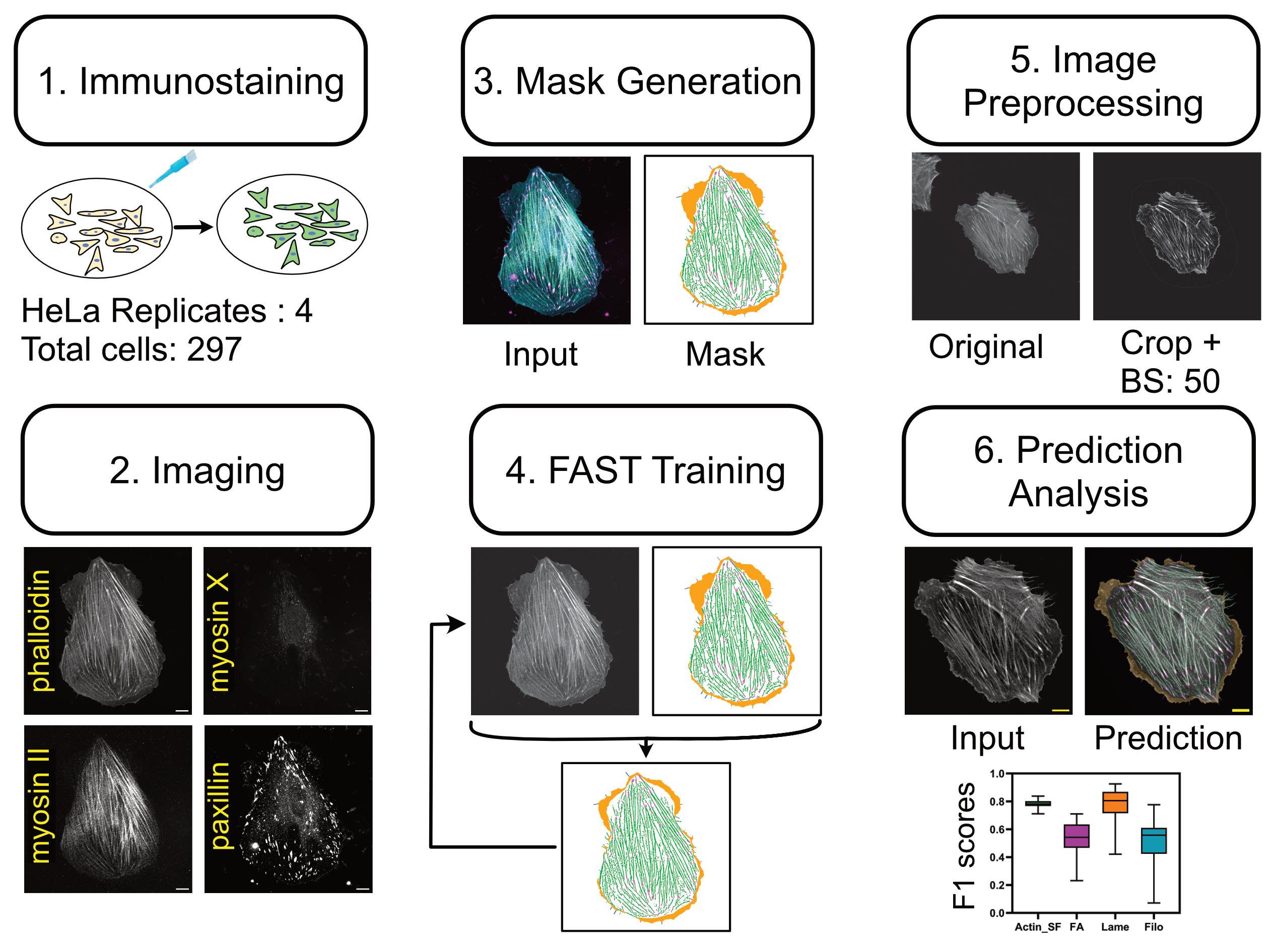
Overview of the pipeline. (1) This tool was trained and validated with confocal microscopy images of HeLa cells that had been fixed and stained with standard immunohistochemistry protocols. (2) Multichannel images with phalloidin, myosin II, myosin X, and paxillin were collected. (3) Masks were created semi-automatically, where phalloidin was used to detect actin and stress fibers (green). The absence of myosin II was used to identify lamellipodia and lamellar regions (orange), the presence of myosin X puncta at the end of thin protrusions was used to detect filopodia (cyan), and paxillin was used to detect focal adhesions (magenta). (4) The phalloidin image and the multilabel mask were used to train FAST. (5) For an unseen dataset, images were preprocessed to remove background (with rolling ball radius 50) and crop single cell prior to inference. (6) Predicted masks based on the phalloidin image alone (Input) can be used as a basis for higher level actin substructure quantification (Prediction) and analysis including F1 scores to measure accuracy (bottom) of actin and stress fibers (Actin_SF, cyan), focal adhesions (FA, magenta), lamellipodia and lamellar regions (Lame, orange), and filopodia (Filo, blue).
Background
Actin is one of the most ubiquitous proteins in eukaryotic cells and is involved in diverse cellular processes, ranging from separating daughter cells during cytokinesis, determining cell shape, mechanotransduction, and driving cell motility [1–3]. This functional versatility is enabled through the dynamic assembly of filamentous actin (F-actin) into diverse higher-order structures, chief of which are lamellipodial and lamellar networks, filopodia, stress fibers, and focal adhesions [4,5]. These structures are mainly defined by their morphology (e.g., lamellipodia and lamellar networks are thin sheet-like extensions, whereas filopodia are finger-like protrusions), the spatial organization of actin filaments in the structure (e.g., stress fibers are formed from bundling of actin filaments), and their association with specific actin regulatory proteins (e.g., focal adhesions, located at sites of contact with the environment surface, contain an array of actin-associated proteins, such as paxillin) [6–9]. Confocal microscopy is well-suited for characterizing the organization of actin filaments into different subcellular structures, where a combination of fluorescently labeled phalloidin with fluorescently conjugated antibodies targeting actin regulatory proteins has been widely used [10]. While this approach can offer high specificity, its effectiveness strongly depends on the quality of the signal and the binding specificity of the antibodies [11]. Additional limitations include the availability of specific antibodies and cross-reactivity arising from shared host species. To address these challenges, we developed a deep learning model, named filamentous actin segmentation tool (FAST), with a unique approach using antibody-assisted labeling, to create high-quality ground truth annotations for detecting multiple classes of actin structures [12]. This protocol details the pipeline used to create datasets that were used to train and validate FAST. The protocol begins with instructions for the preparation of a multichannel dataset by immunostaining and imaging of HeLa cells. While this antibody-assisted annotation approach enables users to generate high-quality custom datasets, we also describe using a pretrained FAST model to quantify the custom phalloidin-stained or live-cell confocal imaging datasets. As part of that, we provide a user-friendly application for fine-tuning image preprocessing parameters.
Materials and reagents
Biological materials
1. HeLa cells (ATCC CCL-2TM)
Reagents
1. Myosin X antibody with mouse host (Novus Biologicals, catalog number: NBP2-88926), store at -20 °C
2. Human myosin IIA (GeneTex, catalog number: GTX33939), store at -20 °C
3. Anti-paxillin antibody (Y113) with rabbit host (Abcam, catalog number: ab32084), store at -20 °C
4. Phalloidin-iFluor 647 reagent (Abcam, catalog number: ab176759), store at -20 °C
5. Goat anti-mouse IgG (H+L) (Alexa Fluor® 405) (Life Technologies Inc, catalog number: A31553), store at 4 °C
6. Goat anti-human IgG (H+L) (Alexa Fluor® 488) (Life Technologies Inc, catalog number: A11013), store at 4 °C
7. Goat anti-rabbit IgG H&L (Alexa Fluor® 568) (Abcam, catalog number: ab175471), store at -20 °C
8. Dulbecco’s modified Eagle’s medium (DMEM) with 4.5 g/L D-Glucose and phenol red (Gibco, catalog number: 11965118), store at 4 °C
9. Phosphate-buffered saline (PBS), 1× with calcium and magnesium (Corning, catalog number: 21-030-CV), store at 4 °C
10. Trypsin-EDTA solution, 0.25% (Gibco, catalog number: 25200056), store at 4 °C
11. Fetal bovine serum (FBS), heat-inactivated (Thermo ScientificTM, catalog number: 10270106), store at -20 °C
12. Penicillin-streptomycin 100× solution (Cytiva, catalog number: SV30010), store at -20 °C
13. PIPES, sodium salt (1.5) reagent grade (BioShop, catalog number: PIP663), store at room temperature
14. Ethylene glycol-bis(2-aminoethylether)-N,N,N',N'-tetraacetic acid (EGTA), ultra-pure, min. 98% (BioShop, catalog number: EGT101), store at room temperature
15. Magnesium chloride (MgCl2) (Quality Biological, catalog number: 351-033-721EA), store at room temperature
16. TritonTM X-100, pH 9.7, non-ionic, liquid (Sigma-Aldrich, catalog number: T8787-50ML), store at room temperature
17. Fibronectin (Corning, catalog number: 354008), store at 4 °C
18. Sucrose (Ward’s Science, catalog number: 470302–808), store at room temperature
19. PierceTM 16% formaldehyde (PFA) (w/v), methanol-free (Thermo ScientificTM, catalog number: 28908), store at room temperature
20. HyCloneTM HyPure water, cell culture grade (Cytiva, catalog number: SH30529.03), store at room temperature
21. Bovine serum albumin (BSA), BioReagent (Sigma-Aldrich, catalog number: A9418), store at -20 °C
22. Sodium azide solution (Sigma-Aldrich, catalog number: 08591-1ML-F), store at 4 °C
Solutions
1. Cell culture medium (see Recipes)
2. Cytoskeletal buffer (see Recipes)
3. Fixing agent (see Recipes)
4. Permeabilization solution (see Recipes)
5. Blocking solution (see Recipes)
6. Sodium azide solution (see Recipes)
7. Primary antibody solution (see Recipes)
8. Secondary antibody solution (see Recipes)
Recipes
1. Cell culture medium
| Reagent | Final concentration | Quantity or volume |
|---|---|---|
| DMEM (+ 4.5 g/L D-Glucose) | 89% | 450 mL |
| FBS | 10% | 50 mL |
| Penicillin-streptomycin | 1% | 5 mL |
| Total | 100% | 505 mL |
Supplement 450 mL of DMEM with 50 mL of heat-inactivated FBS and 5 mL of penicillin-streptomycin. Mix gently to avoid foaming. Store at 2–8 °C for 2–4 weeks. Use sterile technique.
2. Cytoskeletal buffer
| Reagent | Final concentration | Quantity or volume |
|---|---|---|
| PIPES | 80 mM | 1.21 g |
| EGTA | 5 mM | 95 mg |
| MgCl2 | 2 mM | 20.3 mg |
| Culture-grade water | - | 50 mL |
Mix 30–35 mL of dH2O with 1.21 g of PIPES, 95 mg of EGTA, and 20.3 mg of MgCl2. Raise the pH to 6.8 using KOH. Make the final volume of solution to 50 mL by adding dH2O. Sterilize using a 0.22 μm filter. Store at 2–8 °C.
3. Fixing agent
| Reagent | Final concentration | Quantity or volume |
|---|---|---|
| Sucrose | 0.1 g/mL | 1 g |
| Cytoskeletal buffer (Recipe 2) | 0.1× (buffer stock) | 1 mL |
| 16% PFA | 4% | 2.5 mL |
| Culture-grade water | - | 6.5 mL |
Add 1 g of sucrose to 1 mL of cytoskeletal buffer and mix well with 6.5 mL of culture-grade water. Finally, add 2.5 mL of 16% PFA aliquot and mix gently to avoid foaming. Store at 2–8 °C for 2–4 weeks.
4. Permeabilization solution
| Reagent | Final concentration | Quantity or volume |
|---|---|---|
| TritonTM X-100 | 0.1% | 10 μL |
| PBS | - | 10 mL |
Make permeabilization solution by adding 10 mL of PBS to 10 μL of TritonTM X-100. Mix gently to avoid foaming. Store at 2–8 °C for 2–4 weeks.
5. Blocking solution
| Reagent | Final concentration | Quantity or volume |
|---|---|---|
| BSA | 2 mg/mL | 100 μL |
| PBS | - | 10 mL |
Make blocking solution by adding 100 μL of 200 mg/mL BSA stock to 10 mL of PBS and mix gently to avoid foaming. Store at 2–8 °C for 2–4 weeks.
6. Sodium azide solution
Supplement 1 mL of PBS with 1 μL of sodium azide. Store at 2–8 °C for 2–4 weeks. Use sterile technique.
7. Primary antibody solution
| Reagent | Final concentration | Quantity or volume |
|---|---|---|
| Myosin X | 5 μg/mL | 1 μL |
| Myosin IIA | 5 μg/mL | 1 μL |
| Paxillin | 5 μg/mL | 1 μL |
| Phalloidin | 5 μg/mL | 1 μL |
| Blocking solution (Recipe 5) | - | 200 μL |
Make primary antibody solution by adding 1 μL of each of the antibodies listed above to 200 μL of blocking solution and mix gently to avoid foaming.
8. Secondary antibody solution
| Reagent | Final concentration | Quantity or volume |
|---|---|---|
| Goat anti-mouse (Alexa Fluor® 405) | 5 μg/mL | 1 μL |
| Goat anti-human (Alexa Fluor® 488) | 5 μg/mL | 1 μL |
| Goat anti-rabbit (Alexa Fluor® 568) | 5 μg/mL | 1 μL |
| Blocking solution (Recipe 5) | - | 200 μL |
Make secondary antibody solution by adding 1 μL of each of the antibodies listed above to 200 μL of blocking solution and mix gently to avoid foaming.
Laboratory supplies
1. Cell culture flask with filter cap, 25 cm2 (FroggaBio, catalog number: FB-T25-200)
2. 0.22 um PES syringe filter, 25 mm, sterile (FroggaBio, catalog number: SF0.22PES)
3. 8-well chambered cover glass with #1.5 high performance cover glass, 57 mm × 25 mm base (Cellvis, catalog number: C8-1.5H-N)
4. FroggaBio 15 mL conical tubes (rack) (FroggaBio, catalog number: TR15-500)
Equipment
1. Microscope (Nikon Eclipse Ti2 inverted microscope utilizing a CrestOptics X-Light V3 spinning disk integrated with a Photometrics Kinetix camera with 60× 1.2 Numerical Aperture Plan Apo VC water immersion objective)
2. Class II biological safety cabinet (ESCO)
3. CO2 incubator (Thermo Scientific, model: 3110)
4. Freezer, -20 °C
5. Refrigerator, 2–8 °C
Software and datasets
Dataset, model, and software are provided in Table 1 along with version and license information. Additionally, Google Colab notebooks are provided for training to simulate a GUI on a cloud computing platform. Inference and preprocessing are performed with Ilastik [13] and Fiji/ImageJ [14], respectively.
Note: While FAST can be run freely on Google Colab, the availability of GPU resources on the cloud is subject to usage and the subscription type of the user.
Table 1. Software and datasets for data analysis. FAST can be downloaded from GitHub (https://github.com/Carleton-CTE-Lab/FAST-Protocol/archive/refs/heads/main.zip), and the corresponding model link is available on the Google Colab notebook. Dataset is publicly available on Zenodo (https://zenodo.org/records/18135376).
| Type | Software/dataset/resource | Version | Date | License | Access |
|---|---|---|---|---|---|
| Dataset | Zenodo (https://zenodo.org/records/18135376) | V1 | Jan 2, 2026 | Creative Commons | Free |
| Model | Zenodo (https://zenodo.org/records/18627454) | V2 | Feb 13, 2026 | Creative Commons | Free |
| Software | GitHub (https://github.com/Carleton-CTE-Lab/FAST-Protocol) | fast_protocol (tag) | Apr 9, 2026 | MIT | Free |
| Software tool | Fiji/ImageJ (https://imagej.net/software/fiji/) | 2.17.0 | Aug 12, 2025 | GPLv3+ | Free |
| Software tool | Supervisely (https://app.supervisely.com/projects) | 6.15.40 | Dec 23, 2025 | Apache-2.0 | Paid (has free tier) |
| Workflow manager | Ilastik (https://www.ilastik.org/) | 1.4.1.post1 | May 5, 2025 | GPLv3+ | Free |
Procedure
Cell lines were grown in tissue culture flasks with cell culture medium (Recipe 1). Upon reaching ~80% confluency in a 5% CO2 incubator, they were passaged with 0.25% Trypsin-EDTA solution. Prior to the plating, 8-well plates were coated with 10 μg/mL fibronectin in PBS and incubated for at least 15 min. Cells were then re-plated at a lower density and incubated for 6 h in cell culture media (Recipe 1, Figure S1). After plating, users can proceed to the immunostaining steps for generating a labeled training/validation dataset (section A1) or for running only inference with FAST (section A2).
A. Immunostaining procedure
A1. Immunostaining for generating labeled training/validation dataset (optional)
1. Remove cell culture media and fix the cells by gently adding 250 μL of fixing agent (Recipe 3) and incubating for 15 min at 37 °C.
2. Remove the solution and gently wash cells using a pipette three times with PBS.
3. Permeabilize cells with 250 μL of permeabilization solution (Recipe 4) for 20 min at room temperature.
4. Remove the solution and gently wash cells using a pipette three times with PBS.
5. Block cells with 250 μL of blocking solution (Recipe 5) at room temperature overnight to prevent nonspecific antibody binding.
Pause point: If the goal is to use a pretrained model of FAST on a custom dataset, follow section A2 after completing the steps above.
6. Incubate cells with primary antibodies diluted 1:200 in 200 μL of blocking solution (Recipe 5) for 3 h at room temperature:
a. Paxillin (rabbit host)
b. Myosin X (mouse host)
c. Myosin IIA (human host)
7. Remove the primary antibody solution and gently wash cells three times with PBS.
8. Incubate cells with secondary antibodies and phalloidin, each diluted 1:200 in 200 μL of blocking solution, for 1 h at room temperature:
a. Goat anti-mouse IgG (H+L), Alexa Fluor 405
b. Goat anti-human IgG (H+L), Alexa Fluor 488
c. Goat anti-rabbit IgG H&L, Alexa Fluor 568
d. Phalloidin iFluor 647
9. Remove the staining solution and gently rinse cells twice with PBS.
10. Replace PBS with 0.1% sodium azide in PBS prior to imaging for long-term storage of up to 1 week at 2–8 °C.
A2. Immunostaining for inference on phalloidin-stained image dataset
For immunostaining for a custom dataset of phalloidin-stained images, follow the steps in section A1. Then:
1. Incubate cells with phalloidin iFluor 647 diluted 1:200 in 200 μL of blocking solution for 1 h at room temperature.
2. Remove the staining solution and gently rinse cells twice with PBS.
3. Replace PBS with 0.1% sodium azide in PBS prior to imaging for long-term storage of up to 1 week at 2–8 °C.
B. FAST training (optional)
Note: Skip to section C if immunostaining is done by following section A2 to perform inference with the pretrained FAST model. We strongly recommend using Fiji/ImageJ for performing input image preprocessing and mask generation. We also recommend using Google Colab for running the model training script.
1. Following immunostaining in section A1, cells can be imaged in four channels. For the specific antibodies used in FAST and the microscope setup, those parameters are summarized in Table 2. The images were captured at 12-bit 1,600 × 1,600 resolution with a Kinetics camera. Make sure the cell of interest is at the center of the image.
Table 2. Imaging parameters for the antibody-assisted annotation dataset. Metadata from four channel images captured.
| Primary | Secondary | Excitation | Emission | Laser power | Exposure |
|---|---|---|---|---|---|
| Myosin X | Goat anti-mouse (Alexa Fluor® 405) | 365 nm | 438 nm | 80% | 200 ms |
| Myosin IIA | Goat anti-human (Alexa Fluor® 488) | 488 nm | 511 nm | 30% | 200 ms |
| Paxillin | Goat anti-rabbit (Alexa Fluor® 568) | 561 nm | 603 nm | 50% | 200 ms |
| Phalloidin | NA | 640 nm | 685 nm | 2% | 100 ms |
Caution:
1. To avoid photobleaching due to prolonged exposure to high laser power, use the phalloidin channel to select images and acquire them in the following order: phalloidin → paxillin → myosin IIA → myosin X. Avoid unnecessary sample illumination where possible.
2. Please make sure to have prior laser safety training to operate the confocal microscope safely.
2. Masks are generated with a combination of collected image channels. We strongly recommend installing Fiji/ImageJ plugins for this macro. The following preprocessing can also be achieved using the semi_automated_masks Fiji/ImageJ macro provided here. To run the macro, open Fiji/ImageJ: Plugins → Macros → Install → Select “semi_automated_masks.txt.”
a. Actin and stress fiber mask is generated only using the phalloidin channel (Figure 1A) and entails the following major steps:
i. Generating tubeness ensemble mask: Apply Tubeness Plugin with sigma values of 0.8, 1.2, and 1.8 to generate low, medium, and high tubeness images (Figure 1B). Combine all three tubeness images to get an aggregate image with filamentous actin-like structures (Figure 1C).
ii. In addition, skeletonize the phalloidin channel using Fiji/ImageJ function Process → Binary → Skeletonize to obtain a scaffold of actin filaments that can be used to generate filamentous actin class (Figure 1D).
iii. Create an actin class mask based on the intersection of filaments from the tubeness mask and the skeletonized image (Figure 1E).
iv. Finally, apply Analyze → Analyze particles to filter out smaller filament-like noise.
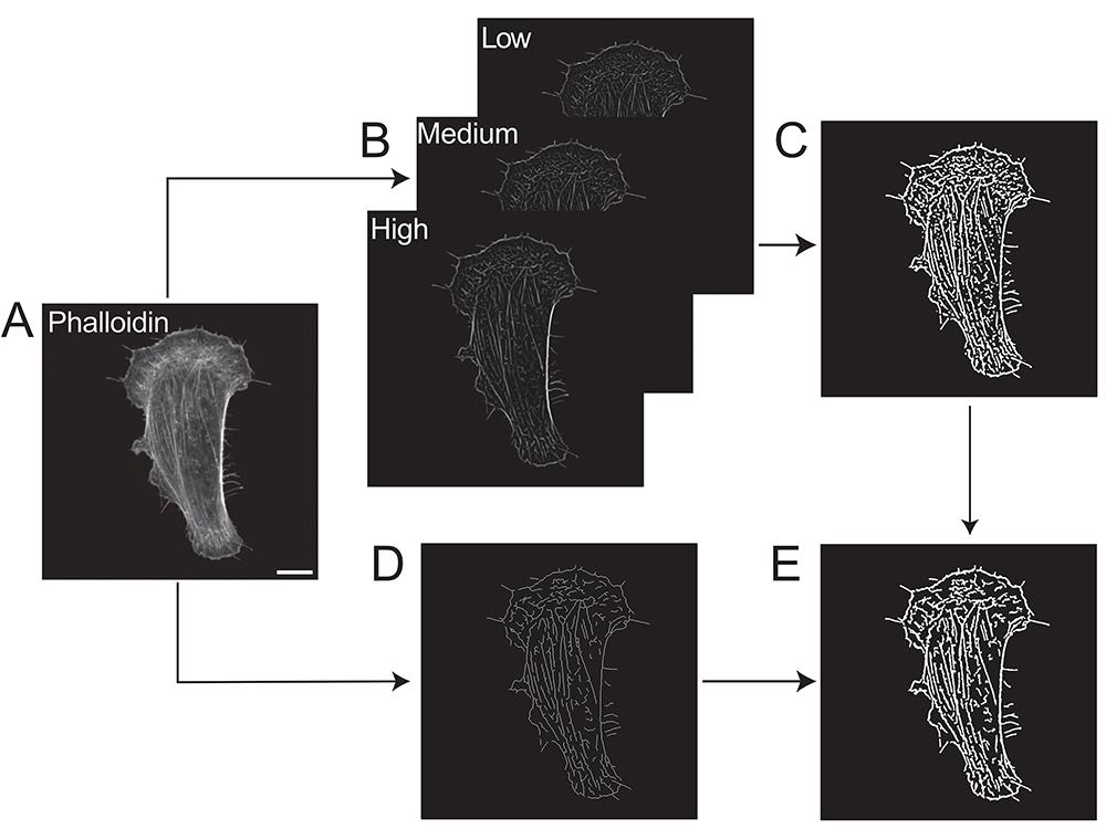
Figure 1. Actin and stress fiber mask generation. (A) The phalloidin channel will be selected by the ImageJ macro provided with the software and applies the tubeness plugin. Scale bar, 10 μm. (B) Three images obtained by applying the tubeness plugin with different diameters. (C) A binary mask is made on the combined image that contains filaments that are seen in all three tubeness images. Additionally, skeletonization is applied on the phalloidin channel to generate the tubeness mask. (D) Scaffold for actin class. (E) Actin and stress fiber mask is obtained by taking the intersection of filaments from the tubeness mask and the skeletonized image.
b. A lamellipodia and lamellar network mask is generated using the phalloidin channel (Figure 2A) and myosin II channel (Figure 2D). This entails the following major steps:
i. Phalloidin mask with morphological opening: The mask from binary thresholding to the phalloidin channel also contains potential filopodia and retraction fibers (Figure 2B). To make sure it is not included in the lamellipodia mask, apply the Morphological opening function of Fiji/ImageJ (Figure 2C) by Plugins → MorphoLibJ → Filtering → Morphological Filters using the Opening operation with Disk Element of Radius 1.
ii. Apply a binary threshold on the myosin II mask (Figure 2E) by Process → Binary → Convert to Mask feature of Fiji/ImageJ.
iii. Create a lamellipodia and lamellar network mask with pixels that are only present in the outer actin mask and not in the inner myosin II mask (Figure 2F).
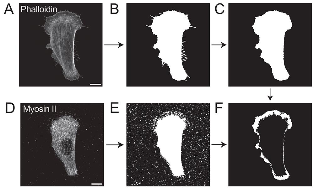
Figure 2. Lamellipodia mask generation from outer and inner masks. (A) Applying thresholding on the phalloidin channel results in (B) a binary mask. (C) Apply morphological opening to this binary mask to get rid of potential filopodia and retraction fibers. (D) Applying thresholding on the myosin II channel results in (E) a binary mask. Subtract the binary mask from myosin II from the binary mask from phalloidin to obtain (F) the mask corresponding to lamellipodia and lamellar regions. Scale bars, 10 μm.
c. The focal adhesion mask is generated using the paxillin channel (Figure 3A) and phalloidin channel (Figure 3C). This entails the following major steps:
i. Thresholding: Apply a binary threshold on the paxillin mask (Figure 3B) by Process → Binary → Convert to Mask feature of Fiji/ImageJ.
ii. Remove puncta at the edges resulting from intensity difference at cell boundaries. For this, create a binary mask following Morphological opening (Figure 3D) and generate cell outlines (Figure 3E).
iii. Remove puncta and boundaries and apply Analyze particles to filter out smaller blob-like noise.
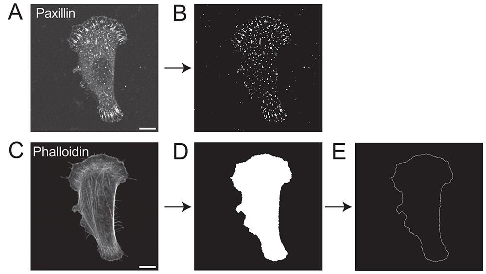
Figure 3. Focal adhesion mask generation. (A) Applying thresholding on the paxillin channel results in (B) a binary mask. (C) Applying thresholding on the phalloidin channel results in (D) a binary mask. Use this cell mask to generate (E) a cell boundary. Scale bars, 10 μm.
d. The filopodia mask is generated using the myosin X channel (Figure 4A) and phalloidin channel (Figure 4D). This entails the following major steps:
i. Apply Thresholding and Analyze particles to the myosin X channel to obtain the initial mask (Figure 4B). Dilate this mask to obtain the myosin X dots mask used for filtering out filopodia-like structures (Figure 4C).
ii. Use the Filoquant plugin of Fiji/ImageJ [15] to obtain all the potential filopodia candidates (Figure 4E).
iii. Selection from potential filopodial candidates is done by iterating over each filopodial candidate from Filoquant and checking if it overlaps with myosin X dots (Figure 4F).
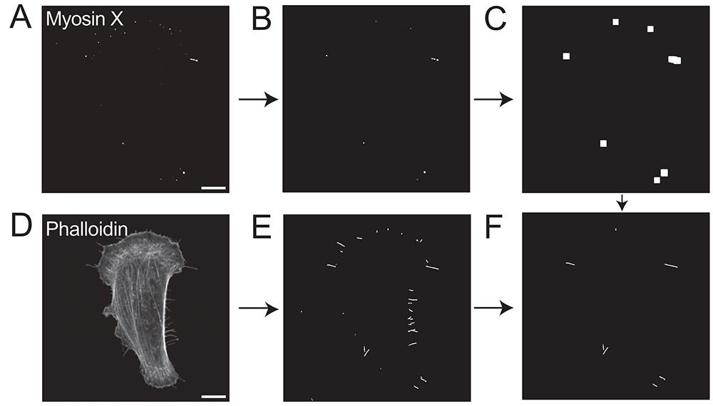
Figure 4. Filopodia mask generation from filoquant and myosin X dots. (A) Apply thresholding to obtain a binary mask from the myosin X channel. (B) Use Analyze particles to select only myosin X dots. (C) Dilate the dots to use as checks for filopodial candidates. Use the phalloidin channel. (D) Mask provided by filoquant to obtain all filopodial candidates. (E) Dilated mask of myosin X dots needs to overlap with a filopodial candidate to be included in (F) the filopodia mask. Scale bars, 10 μm.
Note: When a given pixel is in more than one mask, it is only assigned to one mask based on this priority: actin < focal adhesions < lamellipodia < filopodia.
3. Save the input image after converting it to an 8-bit PNG that has background subtraction and cropped cells for training.
a. Remove the background noise from Channel 4 (phalloidin). This could be done using the background_removal ImageJ macro provided here. To run the macro, open Fiji/ImageJ: Plugins → Macros → Install → Select “background_removal.txt” (see Troubleshooting).
b. Crop the images containing multiple cells or partial cells. This could be done using the selecting_single_cell ImageJ macro provided here. To run the macro, open Fiji/ImageJ: Plugins → Macros → Install → Select “selecting_single_cell.txt” (see Troubleshooting).
4. Open Google Colab in the browser and load the training notebook named fast_training_google_colab.ipynb. If unfamiliar with Google Colab, refer to File S1 for guidance.
5. Once the notebook is loaded, users can find the GUI as shown in Figure 5. For training FAST, provide the link to the folders containing input images of phalloidin with single cells per image and the corresponding multilabel mask image, both as PNGs. Make sure that the input image and the corresponding mask are both 8-bit images saved as PNGs.
6. Click on 1. Setup Colab button to mount the Google Drive and to make sure all the dependencies are installed
7. Click on 2. Start Training button. The code splits the input images and corresponding masks into training, validation, and test sets. Thirty random image mask pairs were selected for validation and test sets. Adjust the training parameters of number of epochs and the number of runs for K-fold cross-validation. The notebooks perform K-fold cross-validation using the dice score and select the model with the best validation score.
8. Evaluate the test dataset with the selected model and use the reported F1 score to adjust the number of epochs and other parameters, such as learning rate (see Result interpretation).
9. Repeat the above steps if necessary and finalize the training parameters.
10. Once the training is completed, the model file corresponding to the best validation score is saved as a .pth file so that it can be downloaded locally. In addition, accuracy metrics, predicted masks, and overlayed masks are also created for visualization of the performance. Click on 3. Download (.zip) button to get the .zip file containing the above files.
Critical: Download the files before re-running the Colab notebook. Having the same file paths will overwrite the previous results.
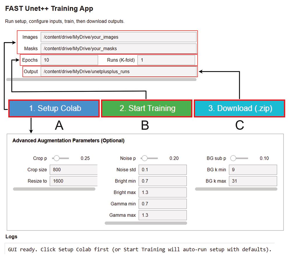
Figure 5. FAST training parameter setup. Upload the separate folders of processed images and corresponding masks in Google Drive and (A) provide the location of images and masks. Change the (optional) advanced data augmentation parameters. (B) Click on 2. Start Training button once all the parameters are set and the text in the logs shows Google Drive to be mounted. Track the training process with text in the Logs box. (C) Upon successful completion of training, the trained model, along with performance metrics on test data, will be available for download by clicking 3. Download (.zip) button.
C. FAST inference
FAST inference is accomplished with the pipeline consisting of setting up the images with preprocessing, loading the model, generating a segmentation mask, and applying the parameters associated with the valid segmentation mask to perform batch inference. The pipeline is detailed below.
1. Following immunostaining with section A2, the cells can be imaged with a single channel of phalloidin. For the specific antibodies used in FAST and the microscope setup, those parameters are listed in Table 2. FAST training and inference images were captured at 12-bit 1,600 × 1,600 resolution with a Kinetics camera. Make sure the cell of interest is at the center of the image.
2. (Optional) Follow step B3b for cropping the cells of interest.
3. Open Ilastik, click on Neural Network Classification (Local) under Segmentation Workflows, and start a new project by providing the location where you would like to save the results. If unfamiliar with Ilastik, refer to File S1 for guidance.
4. Once the GUI is loaded, click on 1. Input Data button to load the test image(s) like the one shown in Figure 6. Ensure that the loaded image is preprocessed with B3a if needed. TIF and PNG are acceptable file formats for this step.
5. Click on 2. NN prediction and type in “reliable-waterbuffalo” in the text box (Figure 6C). Clicking the load button (Figure 6D) will download and initiate the model locally.
Note: The platform only needs to be online for downloading. Alternatively, users can download the model from Bioimage.io and provide the path of the .zip file in the text box to run offline.
6. Click on Live Prediction (Figure 6E) to run the inference locally.
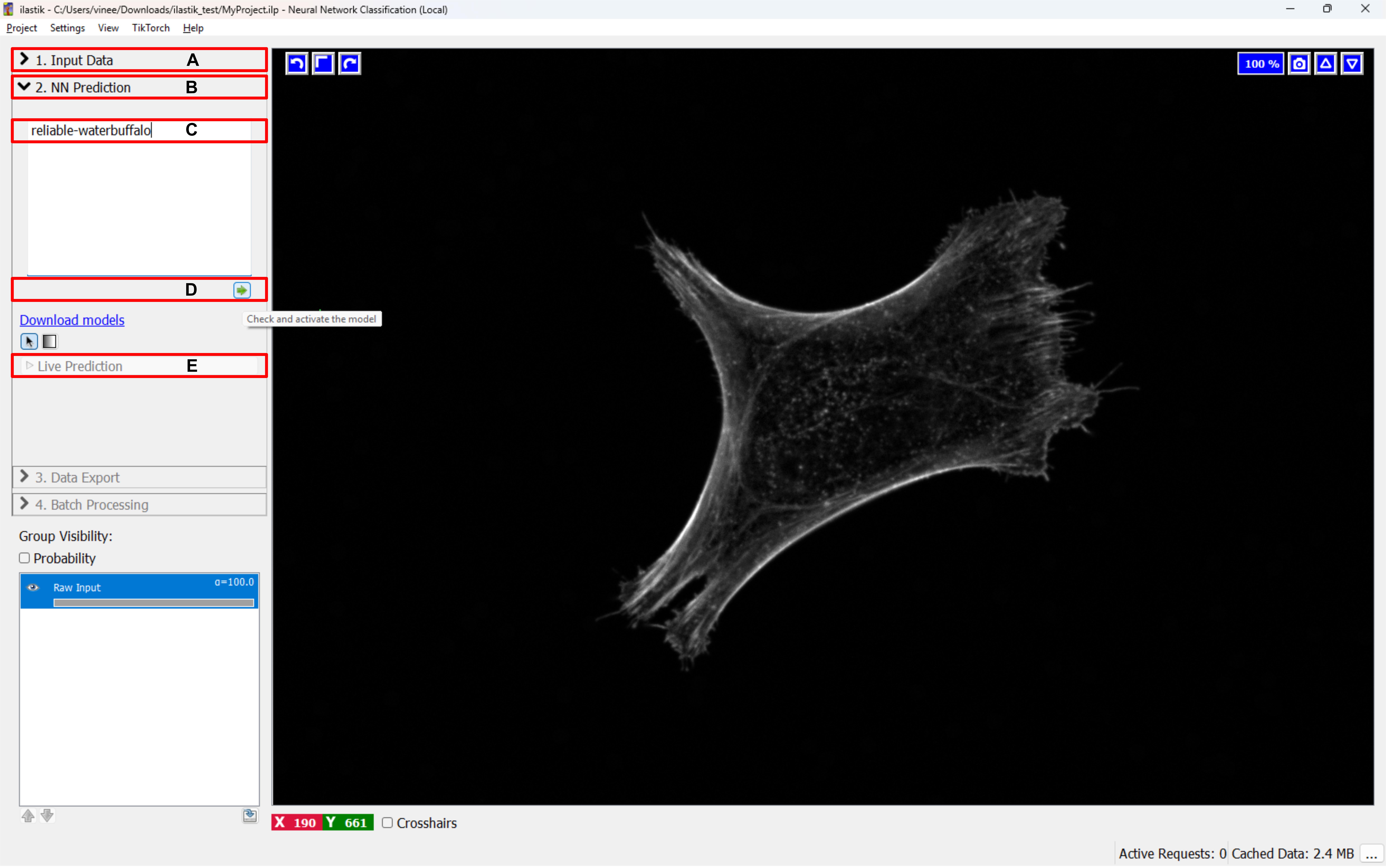
Figure 6. FAST inference model setup. (A) Provide the location of the test image by clicking on 1. Input Data button. (B) Click on 2. NN Prediction button and enter “reliable-waterbuffalo” in the textbox. (C) Click on button (D) to download and initiate the FAST model. (E) Click on Live Prediction to start inference on the test image.
7. Once the inference is done, it is displayed on the GUI, where the user can toggle the input image with the overlayed masks for each class (Figure 7).
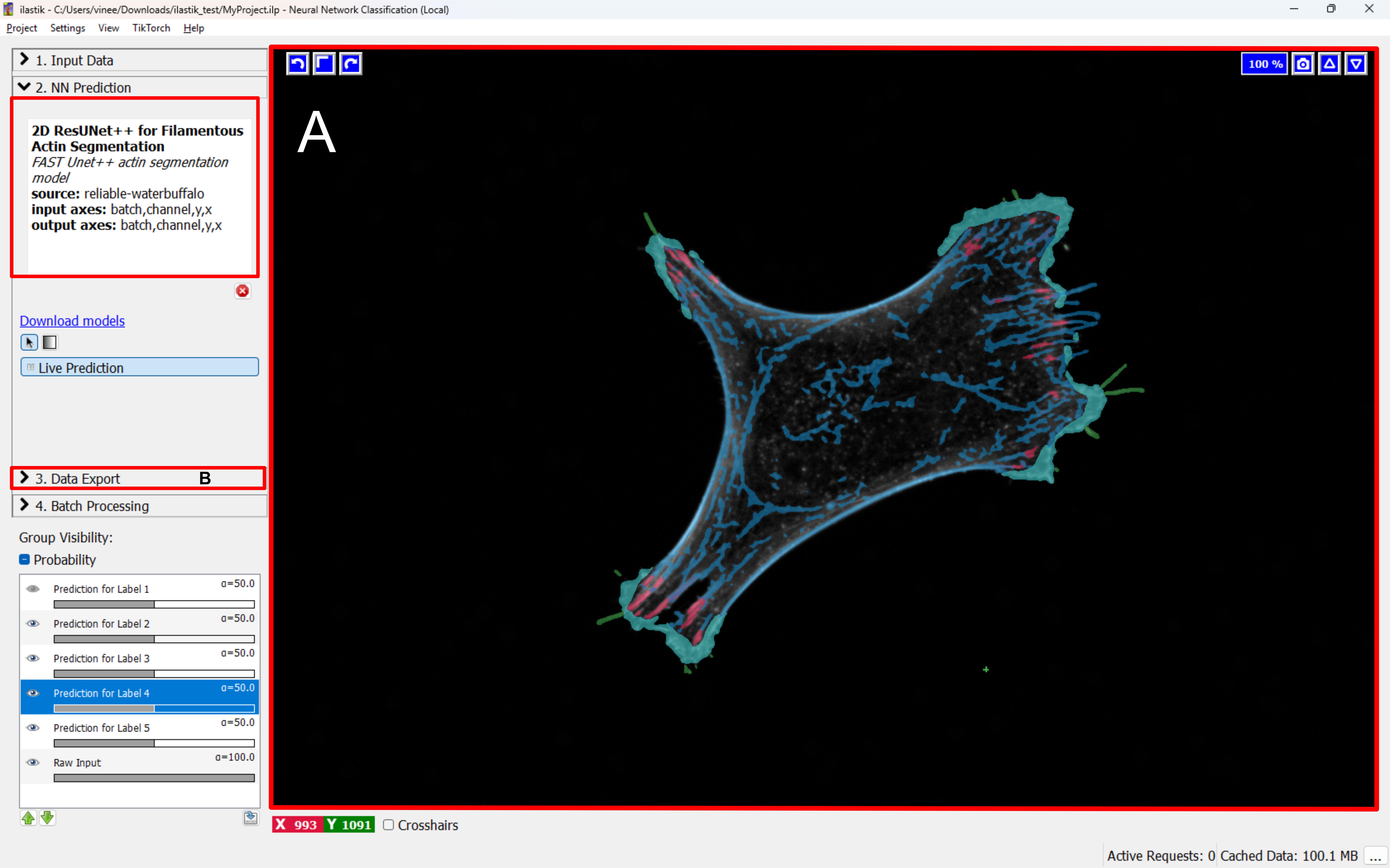
Figure 7. FAST inference with pretrained model. The loaded model is displayed on the left panel. (A) The predicted mask is overlaid with the input image and displayed on GUI. (B) Upon determining the preprocessing, click on 3. Data Export to save the model and inference parameters for batch processing.
8. (Optional) Image signal, background, and quality can influence FAST inference. If the labeling does not look accurate, repeat step B3a with an altered background subtraction radius. The goal is to find the right preprocessing parameters for the custom dataset.
9. Once the prediction on the custom image is confirmed to be valid, click on 3. Data Export to save and load the parameters for batch processing.
10. Once the batch inference GUI loads, select all the images that need to be processed by clicking on Select Raw Data Files (Figure 8). Clicking Process all files will start the batch inference, with the process bar displayed at the bottom.
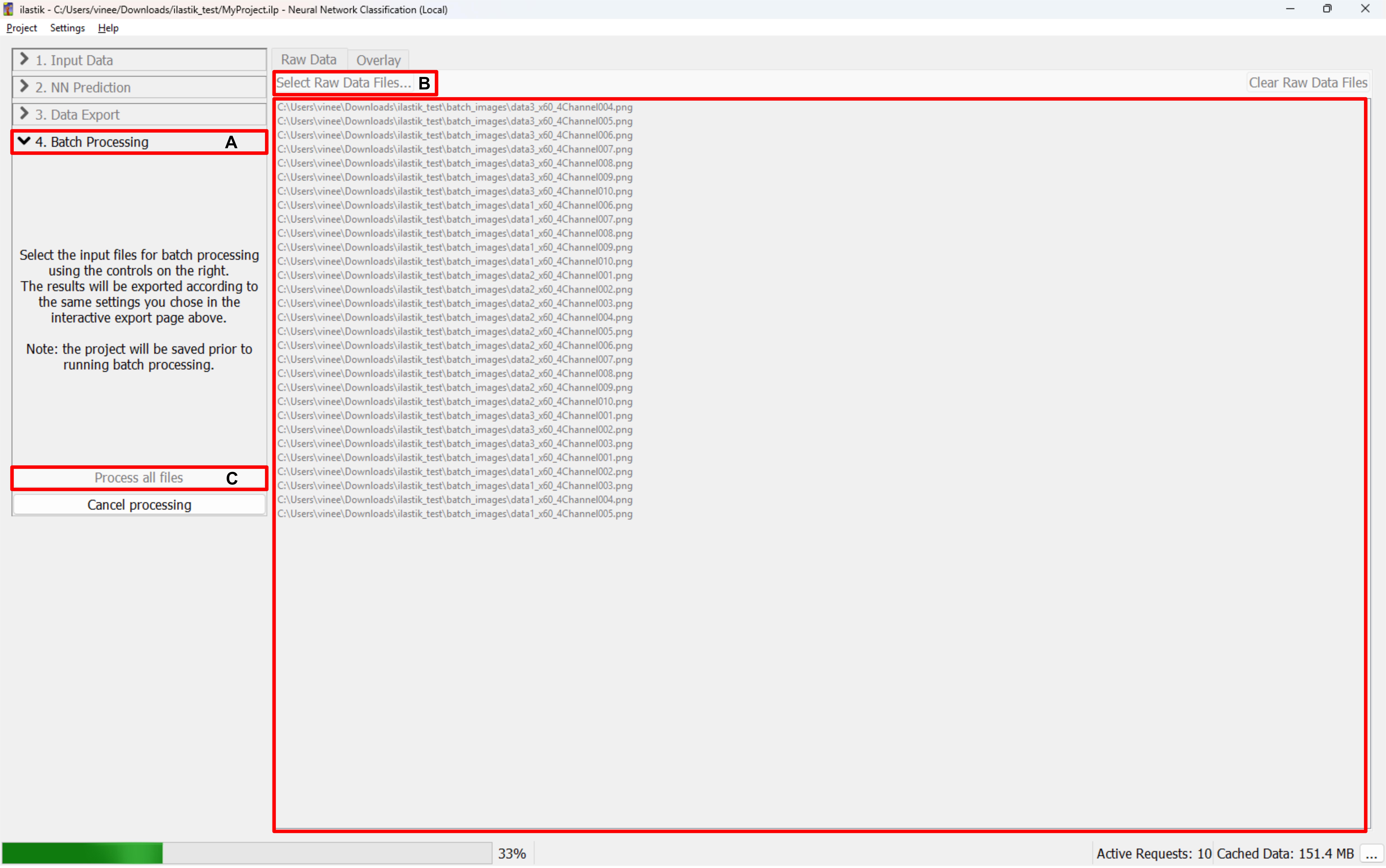
Figure 8. FAST inference in batch mode. (A) Batch process is initiated by clicking 4. Batch Processing and selecting the images to run inference by clicking on (B) Select Raw Data Files…. To start the process, (C) click on Process all files button, upon which the process is shown on the bottom left.
11. Finally, the segmented mask for each of the images in batch inference will be automatically saved as .h5 files in the location provided by the users in step C3 above.
Critical: Download the files before re-running the inference. Having the same file paths will overwrite the previous results.
Data analysis
Result interpretation
FAST is evaluated on three metrics, as follows:
1. Fraction of each class predicted
2. The contour count of each class predicted is obtained from OpenCV (cv2) from the predicted mask (prediction_mask)
for class_label in range(number_of_classes):
class_count = cv2.findContours((prediction[class_label] == class_label), 0, 2)
3. F1-score of each class predicted
Data are presented as mean ± standard deviation. Data were plotted using scatterplots with Pearson’s correlation or box-and-whisker plots with p-values. Statistical analysis was performed using GraphPad Prism or Python. In all cases, p-values < 0.05 were considered significant. For more information, refer to the Statistical analysis section of the FAST paper [12].
Validation of protocol
This protocol has been used and validated in the following research article:
• Aljapur et al. [12]. FAST: Filamentous Actin Segmentation Tool. Journal of Cell Science (Figures 2, 3, and 4)
General notes and troubleshooting
General notes
In general, the performance of segmentation models in image analysis strongly depends on the quality and context of the image data being used, both at the training and inference steps. Below, we provide comments specific to FAST in this regard.
1. FAST was trained on images collected using a spinning disk confocal microscope with a high numerical aperture (NA 1.2) 60× objective. The model might perform best on images collected under similar experimental conditions. The use of FAST for widefield imaging and lower magnifications has not been tested. Users can validate the FAST output for their own imaging setups by comparing output masks to immunostained images, including all the different structures, following the steps described in section A1.
2. In the original manuscript, FAST was tested on adherent cell lines and predicted four classes of actin structure (stress fibers, focal adhesions, lamellipodia/lamellar, filopodia). FAST has not been tested for nonadherent cell lines or for cell lines with a high abundance of other actin structures.
3. Prediction quality of computer vision models, including FAST, mainly depends on the quality of the input image. Specifically, it depends on parameters like signal-to-noise ratio, contrast, extent of photobleaching, and focal plane.
4. Care must be taken to plate the cells at low density, as overlapping cells might lead to incorrect predictions. While this procedure tests for some of the cell lines (of NIH-3T3, HeLa, and LLC-PK1), users could optimize the seeding density according to the cell line for other cell types (see Figure S1).
Troubleshooting
Common problems that might occur during custom image predictions involve missing actin segmentation classes due to a lack of a good signal-to-noise ratio, overlapping cells, and partial cells in the field of view. Images used for FAST analysis should be collected with good signal-to-background and have distinguishable actin structures. Optimize imaging conditions to achieve high-quality images.
Problem 1: The predicted image looks like mostly 1) actin class or 2) lamellipodia class.
Possible cause: The collected image might have excessive cytoplasmic background (see General note 1).
Solution: Adjust the background subtraction radius. See B3a for using the provided ImageJ macro for this solution (Figure 9).
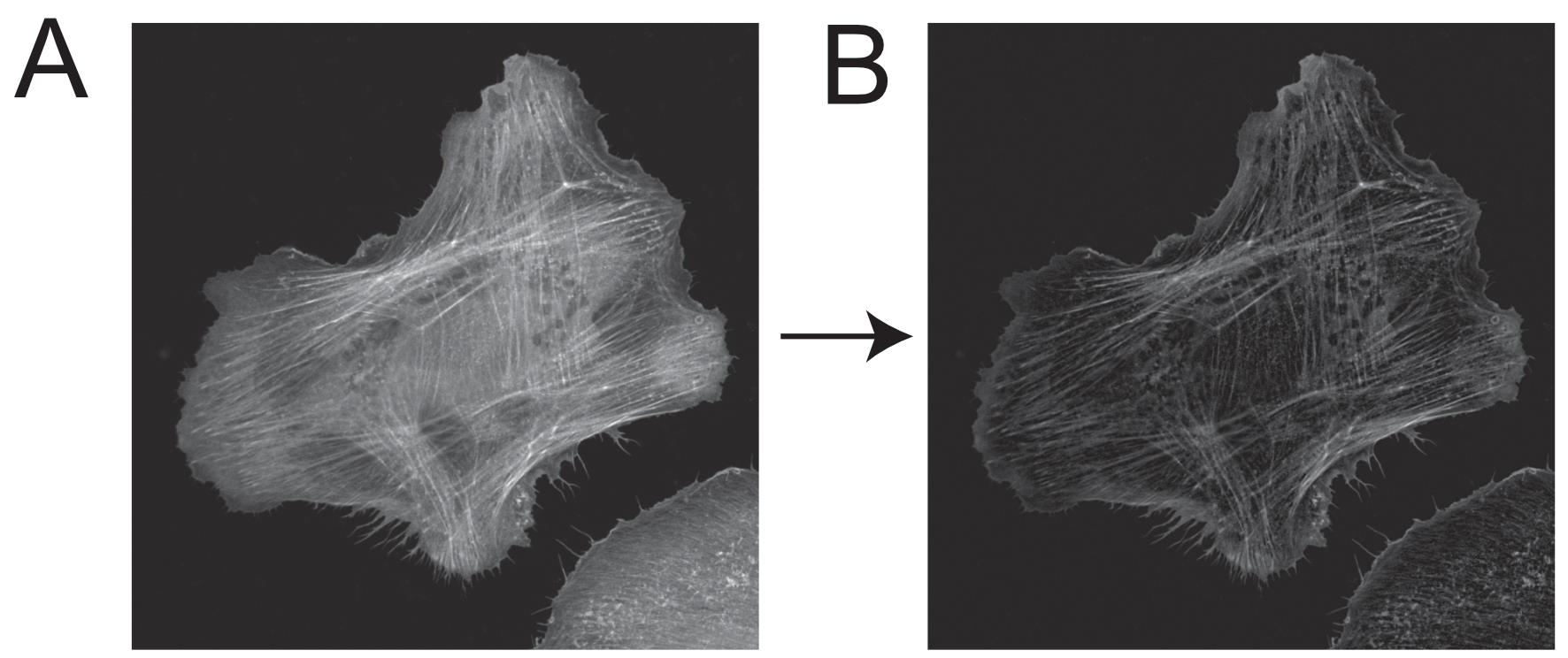
Figure 9. Background subtraction. (A) ImageJ background subtraction was applied to a representative image of HeLa cells. (B) Generating the corresponding background-subtracted image.
Problem 2: Incorrect predictions near the cell edge. 1) Some of the filopodia near the other cells are incorrectly predicted as actin class; 2) some of the actin class is incorrectly predicted as lamellipodia class.
Possible cause: The collected image might have some cells overlapping with the target cell at the center, or some cells might be partially included in the field of view (see General note 2).
Solution: Crop the cells. See step B3b for using the provided ImageJ macro for this solution. The above plugin will give users an option to crop the cell by selecting the freehand tool of ImageJ and making all the pixels outside the cropped polygon to be zero (Figure 10).
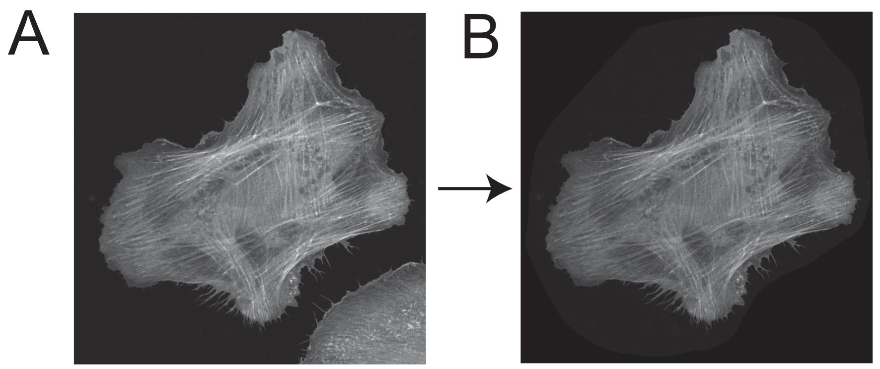
Figure 10. Cropped image of partial cells. (A) ImageJ macro (from step B3b) was applied to a representative image of HeLa cells, (B) generating the corresponding cropped image devoid of partial cells.
Supplementary information
The following supporting information can be downloaded here:
1. File S1. Using Google Colab, Ilastik, and Supevisely.
2. Figure S1. Phase-contrast images of plated cells.
Acknowledgments
All authors were involved in conceptualization of the study. VA performed the experiments and analyzed the data. VA developed the deep learning model and collected training datasets. VA and AH drafted the manuscript. AG and JC provided feedback on model development and implementation. This protocol is adapted from the original work by Aljapur et al. [12]. This work was supported by the OCI-NSERC Alliance grant (OCI# 35778, ALLRP 590443 – 23) and a Banting Foundation Discovery Award to AH. Microscopy equipment used to gather the FAST dataset was supported through a CFI-JELF award and NSERC RTI grant (RTI-2023-00499) to AH. VA was supported by a Vishnu Mehrotra Scholarship and Bhargava Family Scholarship through Carleton University. This research was enabled in part by support provided by Research Computing Services (https://carleton.ca/rcs) at Carleton University.
Competing interests
There are no conflicts of interest or competing interests.
References
- Dominguez, R. and Holmes, K. C. (2011). Actin Structure and Function. Annu Rev Biophys. 40(1): 169–186. https://doi.org/10.1146/annurev-biophys-042910-155359
- Fletcher, D. A. and Mullins, R. D. (2010). Cell mechanics and the cytoskeleton. Nature. 463(7280): 485–492. https://doi.org/10.1038/nature08908
- Pollard, T. D. (2016). Actin and Actin-Binding Proteins. Cold Spring Harbor Perspect Biol. 8(8): a018226. https://doi.org/10.1101/cshperspect.a018226
- Blanchoin, L., Boujemaa-Paterski, R., Sykes, C. and Plastino, J. (2014). Actin Dynamics, Architecture, and Mechanics in Cell Motility. Physiol Rev. 94(1): 235–263. https://doi.org/10.1152/physrev.00018.2013
- Harris, A. R., Jreij, P. and Fletcher, D. A. (2018). Mechanotransduction by the Actin Cytoskeleton: Converting Mechanical Stimuli into Biochemical Signals. Annu Rev Biophys. 47(1): 617–631. https://doi.org/10.1146/annurev-biophys-070816-033547
- Gupton, S. L. and Gertler, F. B. (2007). Filopodia: The Fingers That Do the Walking. Science's STKE. 2007(400): e4002007re5. https://doi.org/10.1126/stke.4002007re5
- Innocenti, M. (2018). New insights into the formation and the function of lamellipodia and ruffles in mesenchymal cell migration. Cell Adh Migr. 12(5): 401–416. https://doi.org/10.1080/19336918.2018.1448352
- Kanchanawong, P., Shtengel, G., Pasapera, A. M., Ramko, E. B., Davidson, M. W., Hess, H. F. and Waterman, C. M. (2010). Nanoscale architecture of integrin-based cell adhesions. Nature. 468(7323): 580–584. https://doi.org/10.1038/nature09621
- Tojkander, S., Gateva, G. and Lappalainen, P. (2012). Actin stress fibers – assembly, dynamics and biological roles. J Cell Sci. 125(8): 1855–1864. https://doi.org/10.1242/jcs.098087
- Desroches, S. and Harris, A. R. (2023). Quantifying cytoskeletal organization from optical microscopy data. Front Cell Dev Biol. 11: 1327994. https://doi.org/10.3389/fcell.2023.1327994
- Kwon, D. (2024). The antibodies don’t work! The race to rid labs of molecules that ruin experiments. Nature. 635(8037): 26–28. https://doi.org/10.1038/d41586-024-03590-0
- Aljapur, V., Gardner, A., Carayanniotis, J. and Harris, A. R. (2026). FAST – filamentous actin segmentation tool for quantifying cytoskeletal organization. J Cell Sci. 139(4): jcs264265. https://doi.org/10.1242/jcs.264265
- Berg, S., Kutra, D., Kroeger, T., Straehle, C. N., Kausler, B. X., Haubold, C., Schiegg, M., Ales, J., Beier, T., Rudy, M., et al. (2019). ilastik: interactive machine learning for (bio)image analysis. Nat Methods. 16(12): 1226–1232. https://doi.org/10.1038/s41592-019-0582-9
- Schindelin, J., Arganda-Carreras, I., Frise, E., Kaynig, V., Longair, M., Pietzsch, T., Preibisch, S., Rueden, C., Saalfeld, S., Schmid, B., et al. (2012). Fiji: an open-source platform for biological-image analysis. Nat Methods. 9(7): 676–682. https://doi.org/10.1038/nmeth.2019
- Jacquemet, G., Hamidi, H. and Ivaska, J. (2019). Filopodia Quantification Using FiloQuant. In E. Rebollo and M. Bosch (Eds.), Computer Optimized Microscopy: Methods and Protocols (pp. 359–373). New York, NY: Springer New York. https://doi.org/10.1007/978-1-4939-9686-5_16
Article Information
Publication history
Received: Apr 13, 2026
Accepted: Jun 9, 2026
Available online: Jun 29, 2026
Published: Jul 20, 2026
Copyright
© 2026 The Author(s); This is an open access article under the CC BY-NC license (https://creativecommons.org/licenses/by-nc/4.0/).
How to cite
Aljapur, V., Gardner, A., Carayanniotis, J. and Harris, A. R. (2026). Actin Quantification Using the Filamentous Actin Segmentation Tool (FAST). Bio-protocol 16(14): e5765. DOI: 10.21769/BioProtoc.5765.

 Download Citation in RIS Format
Category
Bioinformatics and Computational Biology
Cell Biology > Cell imaging > Confocal microscopy
Cell Biology > Cell imaging > Fluorescence
Do you have any questions about this protocol?
Post your question to gather feedback from the community. We will also invite the authors of this article to respond.
 Post a Question


