


- Protocols

- Articles and Issues
- For Authors
- About
- Become a Reviewer


Simultaneous Transcriptomic Analysis of Both Host and Symbiont in Insect–Fungus Interactions


Published: Vol 16, Iss 13, Jul 5, 2026 DOI: 10.21769/BioProtoc.5739 Views: 380
Reviewed by: Lucy XieAnonymous reviewer(s)
 PDF
PDF  Ask a question
Advertisement


Protocol Collections
Comprehensive collections of detailed, peer-reviewed protocols focusing on specific topics




Abstract
In the last two decades, the field of molecular entomology has seen a shift toward next-generation sequencing techniques as a means of uncovering genetic and developmental processes. However, the standardization of methods is not well-established, and studies for insect–fungus consortia lack established protocols for advanced molecular techniques and downstream analysis compared to approaches applied in model systems involving insect–bacteria interactions. To investigate insect–microbe interactions, RNA sequencing and analysis is often used to identify genes involved in the symbiosis. But such protocols do not often consider insect–fungus systems, which vary significantly in community member abundance and/or fail to describe the details of the process from collection to data processing. This paper will introduce a comprehensive approach for RNA sequencing using two non-model insect–fungus consortia, which lack established, published protocols seen in model systems: the ambrosia beetle mutualism and cicada Massospora parasitism. The protocol includes a detailed TRIzol RNA extraction and quantification, RNA sequencing, and data processing using Nextflow pipeline software. Validation of a range of symbiotic interactions from mutualistic to parasitic is considered to justify this procedure to be utilized in a range of insect–fungus interactions with varied abundances and host interactions.
Key features
• Stepwise protocol for RNA extraction of samples containing insect and fungal tissue.
• Novel dissection technique for beetle pupae.
• Acquisition of transcriptomes of both host and symbiont with one protocol.
• Direct comparisons of transcriptomes across life stages, stages of symbiosis, and/or by treatment.
Keywords: Ambrosia beetle Ambrosia Symbiosis
Euwallacea
Fusarium
Massospora
Cicada
RNA Extraction
RNA Seq
Nextflow
Ambrosia Symbiosis
Euwallacea
Fusarium
Massospora
Cicada
RNA Extraction
RNA Seq
Nextflow
Graphical overview
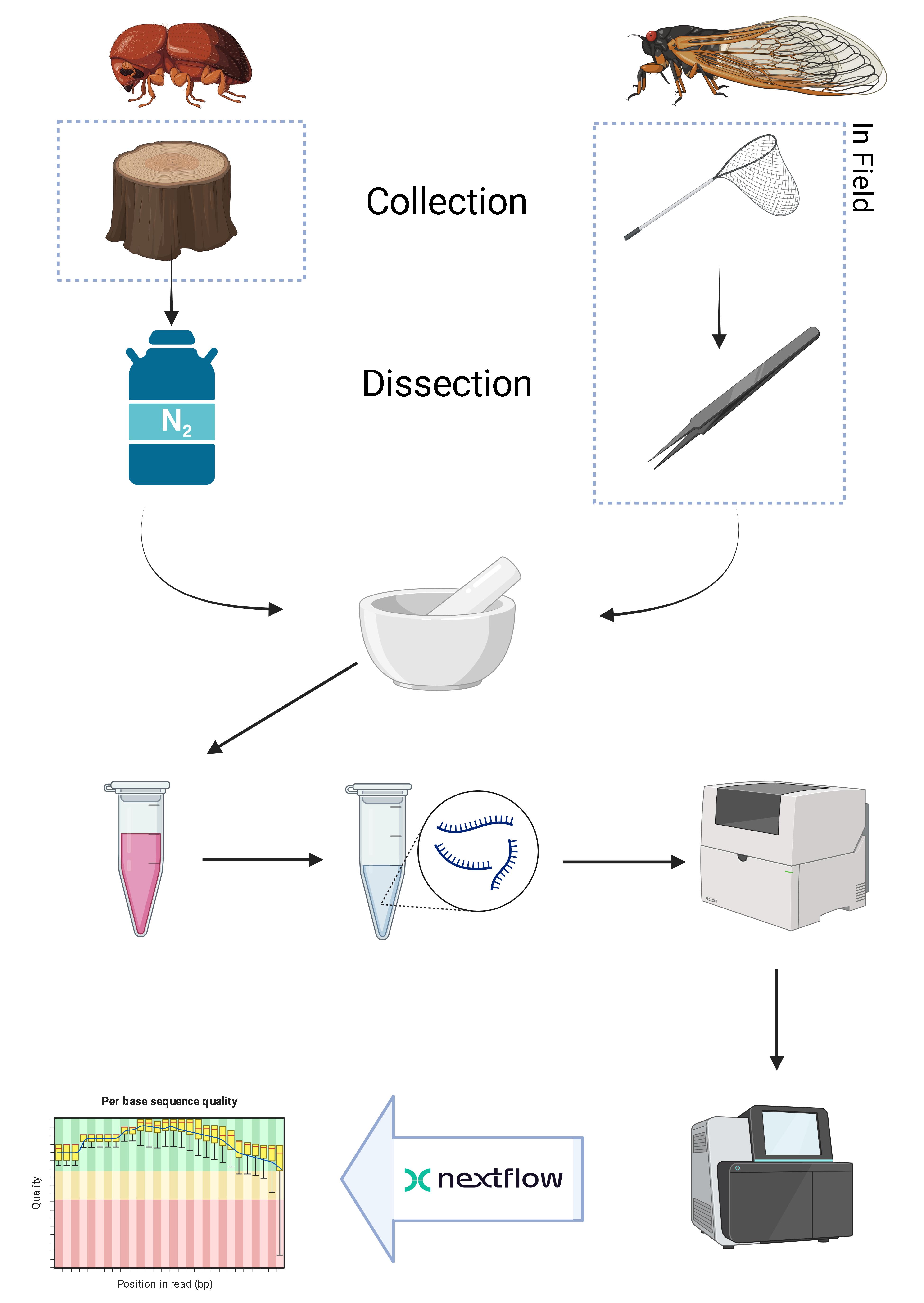
Protocol workflow. Collection methods for ambrosia beetles and cicadas are shown. Then, RNA extraction is shown in general terms: sample preparation, TRIzol extraction, and RNA purification. RNA concentration and quality are measured prior to sequencing. Samples are then analyzed in an Illumina NextSeq 2000 Sequencer. Finally, Nextflow is used to quantify data quality and downstream analysis.
Background
Insect–fungus interactions are ubiquitous in the environment and span the full range of symbiotic interactions, from obligate mutualism to obligate parasitism [1]. One end of the spectrum of symbiosis is obligate mutualism, such as fungus-farming insects, including attine ants (Hymenoptera; Formicidae; Attini), some species of termites (Blattodea; Macrotermitinae), and ambrosia beetles (Coleoptera; Scolytinae and Platypodinae) that engage in behaviors akin to agriculture [2]. Further along the spectrum are insects that still rely on fungi as nutritional sources but lack the specialization seen in the fungus-farming insects; examples of this intermediate mutualism include ship timber beetles (Coleoptera; Lymexylidea), woodwasps (Hymenoptera; Siricidae and Xiphydriidae), and gall midges (Diptera; Cecidomyiidea). Obligate parasitism falls on the opposite side of mutualism on the symbiotic spectrum and includes highly specialized fungal parasites that alter host behavior; these include Cordyceps (Ascomycota; Cordycipitaceae and Ophiocordyceps) and Entomophtora and Massospora (Entomophthoromycota) [3]. A myriad of less specialized facultative fungal pathogens infect insect hosts, making use of the fungal kingdom’s diverse enzymatic abilities to function as pathogens in a range of species. Studies of the molecular mechanisms of these symbioses can inform our understanding of ecology, evolution, and developmental biology, but as these research systems are emerging, they still lack well-established protocols that can be easily adopted and ensure reproducible results.
Determining the genetic and molecular underpinnings of emerging systems comes with a set of challenges not seen in systems with robust molecular procedures. Most insect–fungus systems cannot benefit from established protocols for extensive molecular biology–based research approaches, such as those used in studies of Tribolium and Drosophila [4], due to the range of potential community member abundance between systems. Tribolium and Drosophila have contributed greatly to the fields of developmental biology and genetics, but do not include the unique insect–fungus symbioses. Unfortunately, challenges exist in applying protocols from model systems to non-model systems due to differences in collection, sample composition and morphology, and the question of study [5].
Transcriptomic analysis through RNA sequencing, for example, can be used to determine genetic underpinnings of insect–fungus interactions by sampling at different points in the symbiosis on a temporal or morphological basis. However, insect–fungus samples of different systems will vary significantly in their relative composition of insect and fungal cells and subsequent RNA yields. Consider the following two insect–fungus interactions representing opposite ends of the symbiosis spectrum: The ambrosia beetle Euwallacea validus stores its obligate fungal mutualist Fusarium oligoseptatum in tiny pocket-like organs called mycangia within the head [6,7]. Samples are composed primarily of beetle tissue with relatively few fungal cells, which are aggregated in a discrete location. On the opposite end is the 17-year cicada Magicicada septendecim and its obligate fungal parasite, Massospora cicadina, which consumes and replaces the cicada’s abdomen with fungal spores [8,9]. The remaining “fungal plug” is mostly fungal tissue, while relatively little cicada tissue remains inside in a nonhomogeneous distribution [10].
In hopes of reducing the need for protocols individualized to each system and to promote the study of insect–fungus interactions, a standard transcriptomic analysis workflow for insect–fungus samples of varying composition has been created. These two systems described above, with opposing insect–fungus compositions, were chosen to test the applicability of this protocol across varied sample types representing extreme scenarios. We found that the compositional ratio of fungal tissue to insect tissue did not influence the experimental outcome of this protocol, as RNA extraction of both sample types yielded sufficiently high-quality material that could be sequenced, making it widely applicable across a range of insect–fungus interactions. However, we found that the proportion of transcripts recovered for each partner is dependent on its abundance in the sampled tissues (see Validation, section C).
This protocol is designed to be accessible to all scientists. Price and accessibility of materials were considered. A TRIzol extraction was chosen due to its affordability and applicability to a range of sample types over RNA extraction kits. Two means of quantification are produced. Data processing of RNASeq samples utilizes the open-source workflow and pipeline manager Nextflow [11,12]. Its community and extensive documentation allow its use by those with little to no bioinformatics background. With high accessibility and potential wide application, this protocol aims to bridge the gap of established protocols observed when comparing non-model and model systems, allowing a more effective study of insect–fungus interactions.
Materials and reagents
Biological materials
1. Foundress Euwallacea validus (wild caught: Morgantown, West Virginia, USA, June 2025)
2. Adult periodical cicadas (Magicicada spp.) with conspicuous Massospora cicadina infections (wild caught: Chicago, Illinois, USA, June 2024)
Reagents
1. Nuclease-free H2O (Fisher Bioreagents, catalog number: BP2484-50)
2. 2-propanol, ACS grade (Fisher Chemical, Fisher Scientific, catalog number: A416P-4)
3. RNA-grade ethyl alcohol 200 proof (Pharmco, catalog number: 111000200)
4. TRIzol reagent (Ambion, reference number: 15596018)
5. Chloroform–isoamyl alcohol mixture (Sigma-Aldrich, catalog number: 15593031)
6. Liquid nitrogen (N2)
a. Cold gloves (Tempshield, model: Cryo-Gloves)
b. Cryo bucket for liquid nitrogen
7. RNAlater stabilization solution (ThermoFisher, catalog number: AM7020)
Solutions
1. 70% ethanol (see Recipes)
Recipes
1. 70% ethanol
| Reagent | Final concentration | Volume |
|---|---|---|
| RNA-grade ethyl alcohol 200 proof | 70% | 70 mL |
| Nuclease-free H2O | 30% | 30 mL |
| Total | 100 mL |
Laboratory supplies
1. Supreme air fume hood (Kewaunee Scientific Corporation, model: H07_5472B00)
Note: SME Performance Rating: AI 0.10 ppm.
2. KN95 facemask (multiple manufacturers)
3. Scalpel
4. Aluminum foil
5. Mortar and pestle (cleaned and autoclaved)
Note: Mortar and pestle, 4 inches wide and 3 inches tall, was found to be ideal.
6. Zerotip pipette micro tips 1,000, 200, and 10 μL pipette tips (Biofil, catalog number: PMT371000)
7. 1,000, 200, and 10 μL pipettors (multiple manufacturers)
8. 1.5 mL microcentrifuge tubes (multiple manufacturers)
9. Illumina Stranded mRNA Prep, Ligation Kit (Illumina, catalog number: 20040532)
10. AMPure XP beads for DNA cleanup (Beckman Coulter, product number: A63880)
Note: These are required for the Illumina Stranded mRNA Prep, Ligation Kit.
Equipment
1. High-performance computing cluster
a. The following high-performance computing cluster (HPC) was used for the data analysis contained in this protocol: West Virginia University Research Computing HPC Thorny Flat [specs: 178 compute nodes, 6516 CPU cores, and 47 NVIDIA GPUs; P6000 (21), RTX 6000 (24), A100 (2)]
2. Dell OptiPlex 7060; Intel(R) Core(TM) i7-8700 CPU @ 3.20GHz (3.19 GHz), 64-bit operating system
3. Nanodrop 2000c (Thermo Fisher Scientific, catalog number: ND-2000C)
4. 4200 TapeStation System (Agilent, part number: G2991BA)
5. Microfuge 20R centrifuge (Beckman Coulter, Inc., catalog number: B31612)
6. Freezer
7. Ice and ice bucket
8. Equipment to fell a tree as needed
a. Hand saw or hatchet
b. Chainsaw
Software and datasets
Laboratory device software
1. NanoDrop Operating Software (Thermo Fischer Scientific, v1.2.1); requires registration to download: NanoDrop Product Authentication | Thermo Fisher Scientific - US (access date: 2/10/2026)
2. Tapestation Software (Agilent, v5.2); requires registration to download: Software Download TapeStation Systems | Agilent (access date: 2/10/2026)
Computer software
3. NF-Core RNASeq (Nextflow, v3.21.0); available on GitHub: https://github.com/nf-core/rnaseq.git (access date: 2/10/2026)
4. Miniconda (Anaconda Inc., v25.7.0); available at https://docs.conda.io/projects/conda/en/stable/user-guide/install/index.html (Access date: 2/10/2026)
5. Linux for Windows; Enter “wsl –install” in the terminal (Microsoft Corporation)
Note: XOS and Ubuntu are also compatible with Nextflow and miniconda.
Annotated genomes used for data analysis
Ambrosia beetle head samples:
1. Euwallacea fornicatus (abbreviated hereafter as E. forn; NCBI Genome assembly ASM4011564v1)
2. Euwallacea similis (abbreviated hereafter as E. sim; NCBI Genome assembly ESF131.1)
3. Fusarium oligoseptatum (abbreviated hereafter as F. oligo; NCBI Genome assembly NRRl62579.SpAdes)
4. Fusarium euwallacea (abbreviated hereafter as F. euw; NCBI Genome assembly ASM5061363v1)
5. Raffaelea albimanens (abbreviated hereafter as R. alb; NCBI Genome assembly ASM277824v1)
6. Raffaelea arxii (abbreviated hereafter as R. arx; NCBI Genome assembly ASM277816v1)
7. Raffaelea deltoideospora (abbreviated hereafter as R. delt; NCBI Genome assembly ASM1992538v1)
8. Raffaelea sp. RL272 (abbreviated hereafter as R. spad; NCBI Genome assembly ASM277795v1)
Cicada fungal plug samples:
1. Massospora cicadina (NCBI Genome assembly UCR_MCPNR19_1.0)
2. Magicicada septendecim (NCBI Genome assembly ASM113269v2_)
Procedure
A. Collection and dissection
The following describes the collection and dissection of ambrosia beetles and infected cicadas. The collection will differ from other insect–fungus samples. Keeping to the following principles will ensure your collection goes well. Keep samples free of contamination by handling them with sterile tools, keep them on ice as much as possible to minimize sample degradation, and flash freeze and store as soon as possible. When possible, remove body parts that are not of interest; for example, beetle bodies were not processed, as the fungal mutualist is present in the head. A different ambrosia beetle, however, may store its fungal mutualist in a different location, thus changing the area of interest.
A1. Ambrosia beetle collection
The ambrosia beetle Euwallacea validus was used for this study. Foundresses, female adults in the process of establishing a gallery, were harvested from infested trees in Morgantown, West Virginia, USA, throughout early June of 2025. Trees were monitored, ensuring that foundresses had established galleries within 36 h of collection.
1. Identify an infested tree.
Note: An infested tree can be identified by frass or “sawdust noodles,” evidence of beetles’ boring activity; see Figure 1.
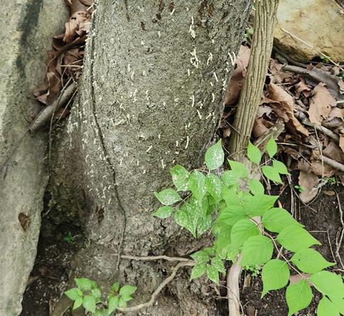
Figure 1. Tree infested with ambrosia beetles. “Sawdust noodles” can be seen when beetles have started gallery initiation.
2. Safely fell the tree and section the infested portions.
a. Trees felled for the purpose of this research were located on West Virginia University campus, and permission was obtained from the Facilities Management Director. When felling and collecting trees, please ensure permission has been granted by the appropriate source, which will depend on land ownership.
Caution: Felling trees is extremely dangerous. Please work with a trained individual to do so.
Note: Tools required depend on tree size. A chainsaw may be required for larger trees.
3. Split the infested section into wedge-shaped pieces. Optimal size is 1 ft long, 30° wedges. Width will depend on the diameter of the tree. Wedges can be cut thinner to access more beetles as needed.
Note: This should be like firewood, but cut thinner; increasing the exposed surface area increases access to beetles (see Figure 2).
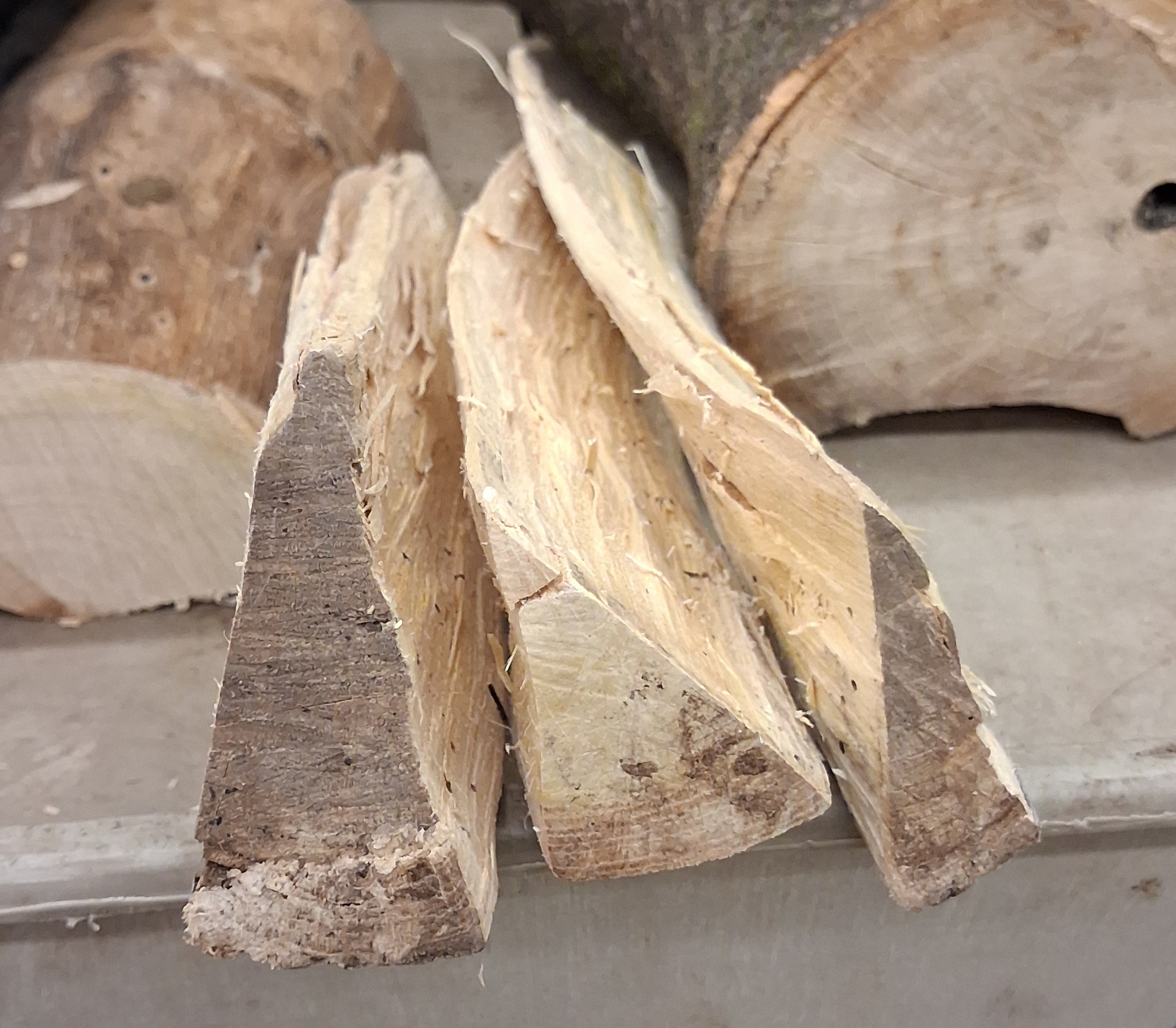
Figured 2. Ambrosia beetle-infested tree sectioned and cut into wedges. Aim for wedges of this size to access all beetles present, especially in highly infested trees.
4. Hit wedge sections against the ground to force out beetles.
Note: The best way to do this is on concrete overlaid with cardboard to better see animals. All life stages can be collected in this way.
A2. Ambrosia beetle pupae dissection
During the pupal stage, internal tissues lose structure and form, becoming liquid. When attempting to dissect a pupa by cutting it, internal tissues spill out and mix. It is then impossible to differentiate between internal tissues with the desired developmental fate. The following method overcomes this issue using liquid nitrogen. When frozen, internal tissues remain in place and do not mix upon dissection.
1. Place one pupa in a 1.5 mL Eppendorf tube.
2. Drop the Eppendorf tube with pupae into the cryo bucket containing liquid nitrogen.
3. With cold gloves, remove after 5 s or when the sizzling sound slows.
Critical: Pupae will come to room temperature quickly. The following steps must be conducted with haste.
4. Drop frozen pupae onto the dissection surface.
Note: A Petri dish lid was used to place the frozen pupae under a dissection scope for higher accuracy during the following step, but this is not necessary.
5. With a scalpel, cut the head off in a single motion.
Note: If timed correctly, the head will easily separate.
6. Place the head in a separate Eppendorf tube on ice.
Note: If possible, dry ice should be used in place of ice.
7. Repeat this for 10 heads.
8. Drop into liquid nitrogen once more to flash-freeze samples.
9. Place in a -80 °C freezer for RNA extraction.
Note: Any time a dissected head spends near room temperature can be considered negative, as cellular breakdown processes can continue. For this reason, only 10 heads are dissected at a time before being placed at -80 °C, where they will remain until RNA extraction. Repeat this process for as many heads as needed.
A3. Cicada collection and dissection
Massospora-infected Brood XIII periodical cicadas (Magicicada spp.) were collected in Glen Ellyn and Lisle, Illinois, on June 5, 2004, and June 6, 2024, respectively. Glen Ellyn collections were from a private residence and included two infected male and two infected female M. septendecim and one infected female Magicicada cassini. Lisle collections included one infected male M. septendecim from the Morton Arboretum (see Figure 3 for an infected cicada). At both locations, infected cicadas were identified and hand collected while wearing nitrile gloves and placed individually inside single 15 mL Falcon tubes with screw caps inside a cooler until processing later that day. In the lab:
1. Remove fungal plugs using a sterile scalpel and forceps and place them in 1.5 mL microcentrifuge tubes containing 500 μL of RNAlater.
2. Let plugs stay at room temperature for 1–2 h to allow RNAlater to fully infiltrate the tissue.
3. Place in a -20 °C freezer for long-term storage.
Note: Flash freezing is not necessary with RNAlater.
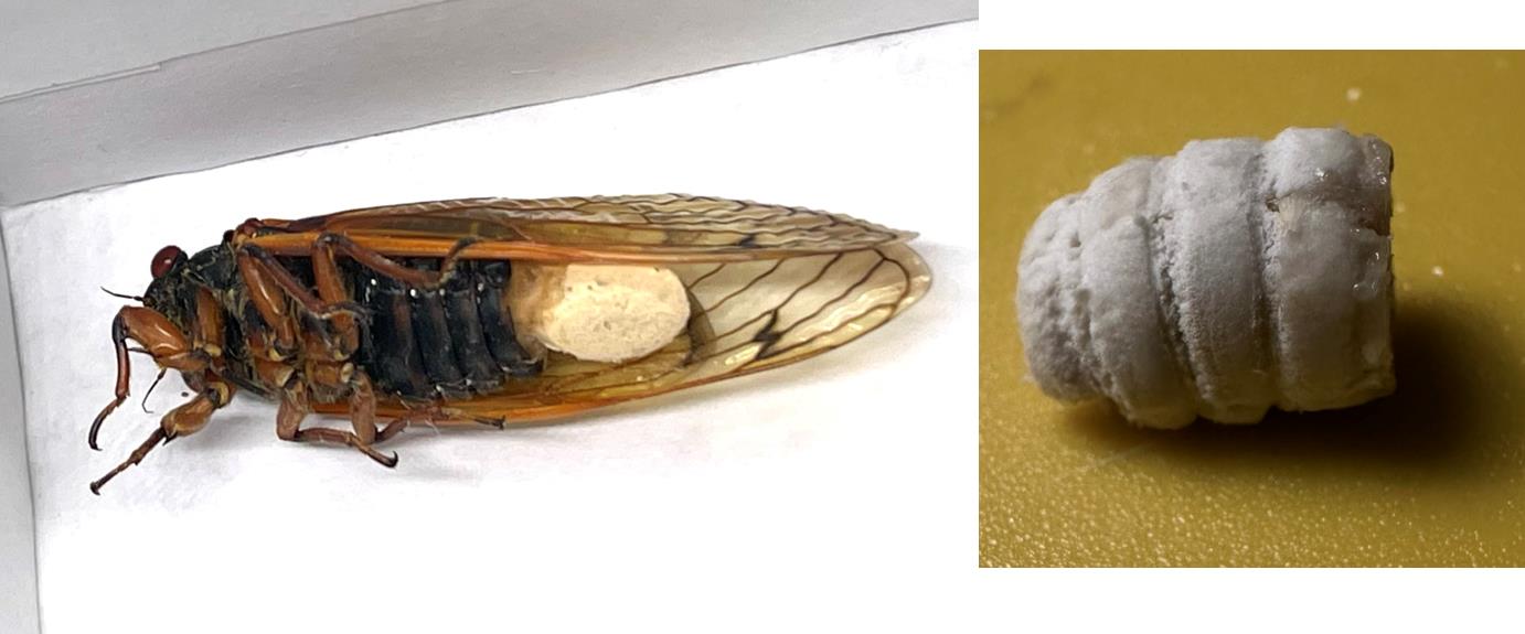
Figure 3. Massospora-infected cicada (left) and fungal plug (right). The fungal plug, still attached to the cicada, is considered to be large, requiring 2 mL of TRIzol.
B. RNA extraction
Throughout the entire protocol, wear a facemask and gloves to protect against harmful reagents, ensure sterile lab conditions, and limit destructive RNase contamination. All following steps, including labeling conventions, are shared by both beetle and cicada samples. For other insect–fungus samples that this protocol can potentially be applied to, steps and labeling conventions do not need to change.
1. Before starting, determine how many milliliters of TRIzol you will need.
Note: More TRIzol results in more RNA extracted from the sample. Too much TRIzol results in a lower concentration and more room for error. In this study, 1 mL of TRIzol was used on 30 ambrosia beetle heads (weighing ~0.1 g), while 2 mL of TRIzol was used on large cicada plugs (weighing ~2 g) and 1 mL of TRIzol on small cicada plugs. This protocol will assume 1 mL of TRIzol.
2. Label a group of 1.5 mL microcentrifuge tubes (equal to the number of milliliters of TRIzol to be used, as determined in step B1) with a “P” and a second set of tubes with “T.” Each milliliter of TRIzol will have corresponding P and T tubes. Labeling is used to denote progress in protocol, rather than sample type or size.
3. Fill a mortar with N2 to cool.
Note: Pour roughly 5 mL of N2 and wait for it to evaporate. Repeat this step three to four times to bring the mortar to the proper temperature.
4. Add the sample.
Note: Flash-freeze samples in N2 prior to this step if not already done.
5. Grind the sample into a fine powder.
Note: Cover with aluminum foil used to autoclave the mortar and pestle when breaking the sample so as not to lose material that may fly out during crushing, as seen in Figure 4.
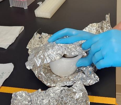
Figure 4. Mortar covered with aluminum foil at the beginning of the grinding process
6. Continue to add N2 incrementally while grinding.
Note: Never allow the sample to dry; a small amount of N2 should always be present.
7. When the sample is a fine powder, add a small amount of liquid nitrogen to the mortar basin. As it evaporates, angle the mortar to concentrate the powdered sample together. Aim to concentrate the sample as shown in Figure 5.
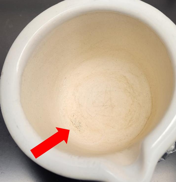
Figure 5. Mortar containing a fully ground sample (highlighted by red arrow), which has been concentrated by tilting
Caution: Move under the fume hood after this step. TRIzol and chloroform are hazardous materials and should only be opened and used under a fume hood.
8. Drip TRIzol onto the sample, 1 mL at a time.
9. Cover all the powdered sample with TRIzol, keeping TRIzol as confined as possible.
Note: Adding TRIzol in a way that decreases surface area covered by TRIzol (least spread around mortar) is best, as it results in the least condensation during warming. When adding TRIzol, pipette out slowly (drip) and angle the mortar with the sample at the bottom, allowing it to freeze on the sample rather than flow off of it. It is advisable to partially add TRIzol, allow it to freeze on the sample, and then add the remaining TRIzol. These conditions allow the best interaction between the sample and TRIzol. Figure 6 provides an example of TRIzol poured with a low surface area.
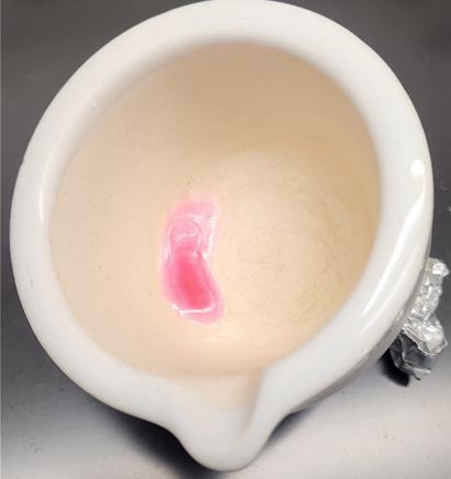
Figure 6. Appropriately poured TRIzol. TRIzol is confined to the sample. Crumbled aluminum foil is used to keep the mortar angled as TRIzol warms.
10. Once thawed, mix by slowly taking the TRIzol–sample mixture up by pipetting within the mortar two times.
11. Add 1 mL of the TRIzol–sample mixture into the corresponding 1.5 mL Eppendorf tube, labeled T.
12. You can drip the mixture on the mortar’s side walls to rinse and collect more sample. Invert to mix 20×.
13. Wait 15 min with samples on ice and invert to mix 10× when removing.
14. Add 200 μL of chloroform to each tube, close them tightly, and invert vigorously 20×. No phase separation is yet seen, as shown in Figure 7.
Caution: Chloroform is a hazardous material; open and use only under a fume hood.
Note: Chloroform tends not to fill the pipette tip to the desired volume. To overcome this, prime the pipette tip headspace: depress the plunger, place the pipette tip into the solution, release to 80% to draw solution into the tip, then depress the plunger to the first stop to evacuate tip volume. Then, pull up 200 μL and proceed with step B14. Take from the bottom layer of the chloroform solution.
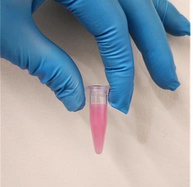
Figure 7. At this step, no phase separation should be seen
15. Wait 15 min with samples on ice.
16. Centrifuge at 15,493× g for 20 min, 30 s at -4 °C.
Note: The required temperature can be reached by placing the centrifuge in a fridge if cooling capabilities are missing. In this case, place equipment in the refrigerator ahead of time to bring the machine's interior to temperature.
17. Move the aqueous layer to tubes labeled P by taking from the top of the aqueous phase, as seen in Figure 8.
Note: During centrifugation, the sample separates into three layers: the clear aqueous phase on top, the white interphase in the middle, and the pink organic phase at the bottom.
Critical: Absolutely do not disturb the interphase or organic phase. Take the aqueous phase in slowly. This is the most important step to obtain high-quality samples. Do not take up any white materials from the interphase layer. 250-400 μL is a sufficient volume of aqueous layer, but aim to recover as much as possible, while disturbing the solution as little as possible.
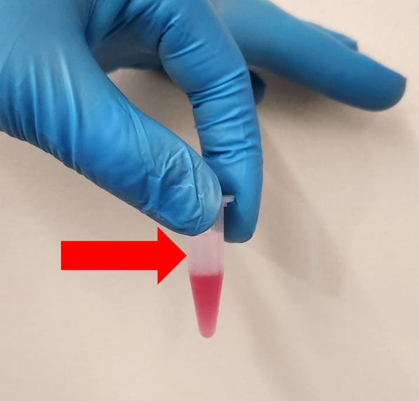
Figure 8. At this step, three phases can be seen
18. Add 500 μL of isopropanol and invert 10×.
19. Place samples at -20 °C (freezer) for ≥30 min.
Note: Samples can sit overnight. This can act as a stopping point.
20. Centrifuge at 15,493× g for 20 min, 30 s at -4 °C.
21. Remove the liquid supernatant by gently aspirating with a pipette.
Note: Typically, an RNA pellet can be seen. It is okay to leave some liquid to avoid disturbing the RNA precipitate. If the RNA pellet is not visible, assume it is present and try to angle the microcentrifuge tube when pipetting to avoid taking it up.
22. Add 500 μL of RNA-grade 70% ethanol to the RNA pellet.
23. Centrifuge at 15,493× g for 5 min, 30 s at -4 °C.
24. Carefully pipette to remove the liquid supernatant.
Note: For cicada plug samples, a second ethanol extraction is performed (repeat steps B22–24).
25. Let the pellet air dry for 3 min.
Note: Leaving the cap open in a fume hood is sufficient.
26. Add nuclease-free H2O for sample resuspension.
Note: The amount of nuclease-free H2O added will depend on the pellet size and further application. A large pellet may accommodate 50 μL of H2O, while nonvisible RNA may benefit from a smaller volume, such as 20 μL.
27. Dissolve RNA: Heat samples lightly at 30 °C for 30 s at a time and tap/flick them every 2 min for 10 min.
28. Label a set of 1.5 mL microcentrifuge tubes, one for each sample, with the sample name, date, and other descriptors for storage. These will hold the final product.
29. Consolidate sample volume from P tubes into the tube labeled in step B28.
30. Freeze overnight at -20 °C before quantification.
C. Quantification
1. Repeat step B27 to redissolve RNA.
Note: Redissolving RNA after freezing overnight results in more accurate measurements.
2. Create a 10× sample dilution for the Nanodrop.
a. Add 1 μL of RNA sample and 9 μL of nuclease-free H2O in a PCR tube.
b. Mix by tapping.
3. Nanodrop:
a. Blank using the same nuclease-free H2O used in step B26.
b. Add 1 μL of diluted RNA sample to the pedestal.
c. Lower the arm and hit Run.
d. Multiply the diluted concentration by 10 to obtain true values.
Note: Values coming from diluted samples will show lower RNA concentration and higher salt concentration than the true sample. Nanodrop is good for a preliminary quality check; a Qubit can be used instead. Prior to running on an RNA sequencing machine, RNA integrity must be quantified on a Tapestation.
4. Tapestation:
a. Gather the required materials: screen tape, buffer, PCR strip, sample, and ladder.
b. Label a PCR strip with sample names, leaving the first tube empty for ladder.
c. Add 10 μL of buffer.
d. Add 1 μL of sample.
e. Repeat for each sample.
f. Add 1 μL of ladder to the first tube.
g. Vortex samples for 5 s and spin down.
Note: A vortexer with a large, flat head was used to vortex all samples in the strip simultaneously.
h. Place the PCR strip into the Tapestation, ensuring that ladder is in column A, row 2. Remove the cap strip.
i. Replace the screen tape.
j. Open the software, select ladder and sample sites, and ensure that the setup onscreen reflects sample placement.
k. Run the program and record the values.
D. Library preparation
Post–RNA extraction, it is typical for samples to be sent to a third-party facility for library preparation and RNA sequencing. However, in this protocol, libraries were produced in-house using the Illumina Stranded mRNA Prep, Ligation kit. The Illumina Stranded mRNA Prep, Ligation kit creates up to 384 unique dual indexes, requires 25–1,000 ng of total RNA, and uses strand orientation to enhance transcript annotation. The manufacturer-provided protocol was followed exactly as described, including the Poly(A) separation step. Buying the kit, along with magnetic beads (required but not included), is an alternative to save labor costs and time. Those capable of executing the RNA extraction protocol above will possess the competency required for this kit.
E. RNA sequencing
After library preparation, samples were sent to Marshall University Genomics CORE for RNA sequencing. Samples were run on an Illumina NextSeq 2000 Sequencer. All runs were paired-end, 100 bp reads. Data was received from Marshall University Genomics CORE through Basespace (Illumina). Following these specific machine and run conditions is not required, but these were used for the samples discussed later in this protocol. Other sequencing machines, such as the Novogene NovoseqX, and conditions, such as single-end reads and 150 bp sequencing depth, are acceptable. At this point in the protocol, quality RNA samples have been produced, allowing the RNASeq machine and run conditions to be determined by the user.
F. Data analysis
The strength of the protocol described thus far lies in its accessibility and reproducibility. To continue this theme, an open-source data analysis workflow that requires minimal starting knowledge was chosen to provide a reproducible and standardized pipeline, with quality documentation. Experience with using Terminal, Linux, environments, and GitHub is recommended. Start by reviewing the “README” document found on the nf-core/rnaseq GitHub page (see Computer software) [12]. Nextflow offers training (https://training.nextflow.io/2.1.1/) and has a series of YouTube videos to follow along with to get started, found here [11]. The “Hello Nextflow” and “Nextflow for RNAseq” will be your starting point. All samples in this study were processed using the nf-core/rnaseq pipeline by Nextflow. The following section will contain a step-by-step guide for installing and using Nextflow. The following data analysis was done using WVU’s high-performance computing cluster. This protocol will work with any HPC, although gaining access and activation on the command window will differ by organization.
F1. Download and install all dependencies
1. Windows users must install Linux for Windows.
a. Open the Terminal and type “wsl –install.” Hit enter.
b. You will be prompted to close the terminal; do so to continue.
c. Moving forward, when using the terminal, type “wsl” and hit enter to start working in Linux.
Note: As stated in the software section, XOS and Ubuntu can substitute Linux for Windows.
2. Create a project folder.
a. It is common practice to create a working folder that will be used for the entire project and will hold all data and result files. Create a folder and move all required data files to this path (RNASeq files and genomic data).
b. If this was not done in the command window, open the command window.
c. Change your working directory to the folder you just made.
3. Install Conda
a. Conda is an “environment” manager. In simple terms, an environment in this context creates a separate instance of your computer that is partitioned from other processes, like using a different desktop on the same computer, where certain files can be stored and used. It is recommended that each project has its own environment to keep all dependencies together.
b. Install Conda. The installation link and guide can be found above in Software and Datasets (Anaconda Inc.).
c. Add channels and ensure correct order, type the following into the command window, and hit enter after each.
conda config --add channels biocondaconda config --add channels conda-forgeconda config --set channel_priority strictF2. Connect to a high-performance computing cluster
The process of gaining access and activating on a command window to a high-performance computing cluster will differ by organization.
Note: Your organization and HPC provider may require an SSH manager. Putty can be installed for free from the Microsoft Store.
After accessing your institutions’ HPC and connecting to it, create an active session and activate conda.
srun --pty bashmodule load condasource /shared/software/conda/conda_init.shYour command prompt line should now note that you are in an active HPC session.
Note: srun –pty bash allocates a predetermined amount of resources; this can be changed.
F3. Create an nf-core/RNASeq Environment
1. Use the information above to connect to an HPC and set the working directory to your Project Folder.
2. Creating a new environment. Downloading Nextflow and its dependencies can be done with the following commands:
conda create --name env_nf env_nf/rnaseq Nextflowconda activate env_nf3. You should see (env_nf) appear to the left of your command line prompt. This means your new environment, env_nf, is active. This environment contains Nextflow and will be used for data analysis.
Note: Using conda is one of several ways to accomplish this. Singularity and Docker are commonly used environment managers that will perform the same requirements as conda.
F4. Run Nextflow
1. Log onto your HPC and activate a session, activate conda, and activate the environment with Nextflow.
2. Create a sample sheet.
a. Create a comma-delimited .csv file with the following headers: sample, fastq_1, fastq_2, strandedness.
b. Each row will contain related information for a single sample, e.g., BH1, BH1.R1.fastq.gz, BH1.R2.fastq.gz, auto.
3. Create a BBSplit list.
a. Each genome will have one line containing the following: Genome, path/to/genome.gz.
b. Save as “bb_split_list.txt.”
4. To utilize BBSplit, add the following to the Nextflow run command:
a. –bbsplit_fasta_list bb_split_list.txt \
b. –skip_bbsplit false \
Note: You can familiarize yourself with Nextflow through their YouTube videos: https://youtube.com/playlist?list=PLPZ8WHdZGxmWKozQuzr27jyMGqp9kElVK&si=-SycOsiC6S6F39lW.
Nextflow can now be run, adding parameters as necessary.
F5. Example code
1. Download genomes:
#!/usr/bin/bash -l#SBATCH -p shortmkdir -p genomepushd genomecurl -O https://ftp.ncbi.nlm.nih.gov/genomes/all/GCA/003/946/995/GCA_003946995.1_NRRL62579.SPAdes/GCA_003946995.1_NRRL62579.SPAdes_genomic.fna.gzcurl -O https://ftp.ncbi.nlm.nih.gov/genomes/all/GCA/003/946/995/GCA_003946995.1_NRRL62579.SPAdes/GCA_003946995.1_NRRL62579.SPAdes_genomic.gff.gzcurl -O https://ftp.ncbi.nlm.nih.gov/genomes/all/GCA/003/946/995/GCA_003946995.1_NRRL62579.SPAdes/GCA_003946995.1_NRRL62579.SPAdes_genomic.gtf.gzgunzip *.gzln -s GCA_003946995.1_NRRL62579.SPAdes_genomic.fna Fusarium_oligoseptatum_NRRL_62579.fastaln -s GCA_003946995.1_NRRL62579.SPAdes_genomic.gtf Fusarium_oligoseptatum_NRRL_62579.gtfln -s GCA_003946995.1_NRRL62579.SPAdes_genomic.gff Fusarium_oligoseptatum_NRRL_62579.gffrsem-gff3-to-gtf --RNA-patterns mRNA,rRNA Fusarium_oligoseptatum_NRRL_62579.gff Fusarium_oligoseptatum_NRRL_62579.fixed.gtfperl -i -p -e 's/rna-gnl\|WGS:NKCK\|//' genome/Fusarium_oligoseptatum_NRRL_62579.fixed.gtfcurl -O https://ftp.ncbi.nlm.nih.gov/genomes/all/GCF/040/115/645/GCF_040115645.1_ASM4011564v1/GCF_040115645.1_ASM4011564v1_genomic.fna.gzcurl -O https://ftp.ncbi.nlm.nih.gov/genomes/all/GCF/040/115/645/GCF_040115645.1_ASM4011564v1/GCF_040115645.1_ASM4011564v1_genomic.gff.gzln -s GCF_040115645.1_ASM4011564v1_genomic.fna.gz Euwallacea_fornicatus_EFF26.fna.gzln -s GCF_040115645.1_ASM4011564v1_genomic.gff.gz Euwallacea_fornicatus_EFF26.gff.gz2. Nextflow run:
#!/usr/bin/bash -l#SBATCH -p epyc -n 1 -N 1 -c 24 --mem 192gb --out logs/nf.log --time 3-0:0:0module load singularityGENOME=genome/Fusarium_oligoseptatum_NRRL_62579.fastaGTF=genome/Fusarium_oligoseptatum_NRRL_62579.fixed.gtfGFF=genome/Fusarium_oligoseptatum_NRRL_62579.gffmkdir -p resultsnextflow run nf-core/rnaseq -resume -c ucr_hpcc.config -profile singularity \ --input samplesheet.csv \ --bbsplit_fasta_list bb_split_list.txt \ --skip_bbsplit false \ --outdir results/nf_rnaseq \ --gtf $GTF \ --fasta $GENOME \ --star_rsem --save_unaligned \ --minAssignedFrags 1 \ --skip_pseudo_alignment3. Assign reads with BBSplit:
#!/usr/bin/bash -l#SBATCH -p shortmkdir -p genomepushd genomecurl -O https://ftp.ncbi.nlm.nih.gov/genomes/all/GCA/003/946/995/GCA_003946995.1_NRRL62579.SPAdes/GCA_003946995.1_NRRL62579.SPAdes_genomic.fna.gzcurl -O https://ftp.ncbi.nlm.nih.gov/genomes/all/GCA/003/946/995/GCA_003946995.1_NRRL62579.SPAdes/GCA_003946995.1_NRRL62579.SPAdes_genomic.gff.gzcurl -O https://ftp.ncbi.nlm.nih.gov/genomes/all/GCA/003/946/995/GCA_003946995.1_NRRL62579.SPAdes/GCA_003946995.1_NRRL62579.SPAdes_genomic.gtf.gzgunzip *.gzln -s GCA_003946995.1_NRRL62579.SPAdes_genomic.fna Fusarium_oligoseptatum_NRRL_62579.fastaln -s GCA_003946995.1_NRRL62579.SPAdes_genomic.gtf Fusarium_oligoseptatum_NRRL_62579.gtfln -s GCA_003946995.1_NRRL62579.SPAdes_genomic.gff Fusarium_oligoseptatum_NRRL_62579.gffrsem-gff3-to-gtf --RNA-patterns mRNA,rRNA Fusarium_oligoseptatum_NRRL_62579.gff Fusarium_oligoseptatum_NRRL_62579.fixed.gtfperl -i -p -e 's/rna-gnl\|WGS:NKCK\|//' genome/Fusarium_oligoseptatum_NRRL_62579.fixed.gtfcurl -O https://ftp.ncbi.nlm.nih.gov/genomes/all/GCF/040/115/645/GCF_040115645.1_ASM4011564v1/GCF_040115645.1_ASM4011564v1_genomic.fna.gzcurl -O https://ftp.ncbi.nlm.nih.gov/genomes/all/GCF/040/115/645/GCF_040115645.1_ASM4011564v1/GCF_040115645.1_ASM4011564v1_genomic.gff.gzln -s GCF_040115645.1_ASM4011564v1_genomic.fna.gz Euwallacea_fornicatus_EFF26.fna.gzln -s GCF_040115645.1_ASM4011564v1_genomic.gff.gz Euwallacea_fornicatus_EFF26.gff.gzNote: Scripts were deposited in the following GitHub: https://github.com/stajichlab/KassonLab_Mycangium_RNAseq.
Validation of protocol
The innovation of this protocol is the ability to produce high-quality RNA for RNA sequencing from a range of insect–fungal consortia in situ. E. validus and Massospora cicada samples are expected to contain both host and fungal symbiont transcripts, while differing significantly in their composition. Ambrosia beetles with fungal pockets represent discrete symbiont tissues, while cicadas consumed by fungal tissue represent heterogeneous, non-discrete sample composition. 11 samples were processed for the validation of this protocol: six fungal plugs recovered from infected cicadas (C1–6) and five groups of pooled (30/group) beetle heads (BH1–5). Twenty-two FASTQ.gz files were received, two for each sample due to paired-end reads. Validation of this protocol requires two things: evidence that extracted RNA is of high quality, and the detection of both host and symbiont transcripts in both sample types.
RNA quality is shown below in Table 1 at three steps: Nanodrop, Tapestation, and FastQC measurements. The pipeline manager Nextflow utilizes BBSplit to confirm the presence of both host and symbiont in both sample types by mapping to two reference genomes simultaneously. Table 1 below shows Nanodrop and Tapestation data. Nanodrop data show that all samples have concentrations in ranges acceptable for library creation (≥200 ng/μL). Given that the samples are dilutions of the product, 260/280 values, which determine RNA purity based on protein contamination, will appear lower than the true value. Yet, an acceptable range of 1.75 ≤ × ≤ 2.15 is maintained. Several 260/230 values are below the desired target range of 2.0–2.2. This can be explained by the use of dilutions on the Nanodrop rather than the true sample, which amplifies the signal of contaminants. Further processes during the library preparation step aid in reducing the contaminants detected by the 260/230 Nanodrop ratio. All Tapestation RNA integrity number equivalent (RINe) values indicate that RNA within all samples is of high quality and at low degradation levels, as seen in Table 1, with RINe ≥ 8 representing a high-quality sample.
Table 1. NanoDrop and Tapestation values for all samples
| Nanodrop | Tapestation | |||
| (ng/μL) | 260/280 | 260/230 | RINe | |
| BH1 | 225 | 1.81 | 0.83 | 9.2 |
| BH2 | 350 | 1.78 | 1.38 | 8.0 |
| BH3 | 216 | 1.91 | 1.71 | 8.0 |
| BH4 | 260 | 1.76 | 1.39 | 8.2 |
| BH5 | 478 | 1.83 | 1.32 | 9.8 |
| C1 | 950 | 2.05 | 2.50 | 9.4 |
| C2 | 1150 | 2.11 | 2.14 | 8.3 |
| C3 | 410 | 1.95 | 0.92 | 9.7 |
| C4 | 1030 | 1.97 | 1.20 | 9.1 |
| C5 | 345 | 1.85 | 0.63 | 9.5 |
| C6 | 600 | 1.90 | 0.68 | 9.6 |
Per base sequence quality from the FastQC-generated report for sample BH1 is shown in Figure 9, showing a score of 38-39/40 for all read positions. No box or whisker plots can be seen due to the statistically insignificant variability at each read position. This indicates extremely high-quality RNA within a sample. Sample BH1 was chosen only because it is the first sample, as all other samples have a similar per base sequence quality plot.
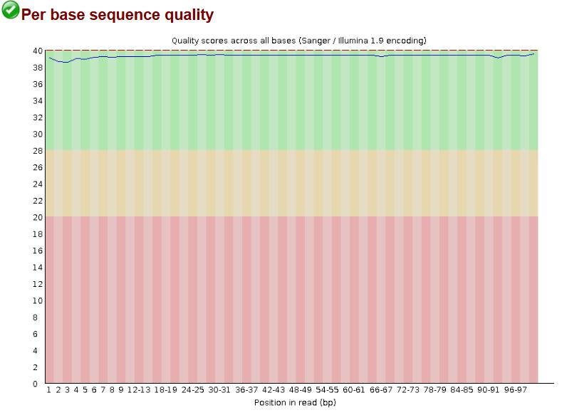
Figure 9. FastQC per base sequence quality output for sample BH1
Finally, Figures 10, 11, and 12 explore the mapping of reads to each genome. Figure 10 shows the proportion of reads mapped to host and fungal partner and unmapped reads in both the cicada–Massospora and Euwallacea–Fusarium symbioses. In both cases, the proportion of mapped reads aligns with expected outcomes based on tissue concentration and distribution. Based on estimates from µCT imaging, mycangia represent a volume of 0.34 mm3, while heads are 4.2 mm3, with 1% of fungal transcripts aligning with the expected ratios of fungal-to-beetle tissues. The quantity of cicada tissues within fungal plugs cannot be directly observed; however, most cicada tissues are assumed to have been consumed by the fungal parasite. 7% of cicada transcripts align with expected ratios of fungal and cicada tissues. Results within Figure 10 demonstrate that this protocol can successfully detect transcripts for both partners of an insect–fungi symbiosis, regardless of tissue homogeneity, status of symbiosis, or ratios of tissues within the sample.
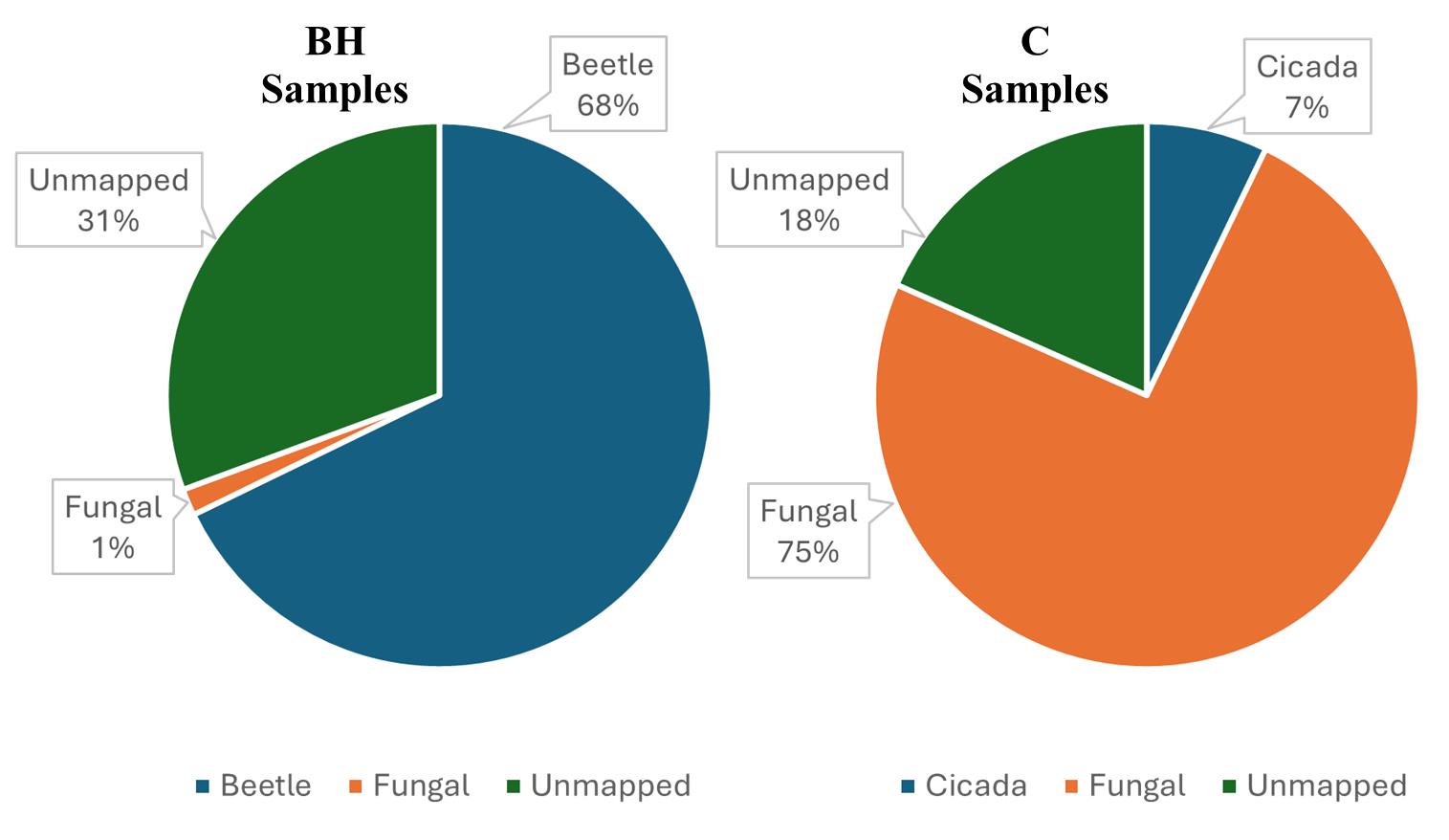
Figure 10. Percent of transcripts mapped to host, fungal symbiont, or unmapped in Euwallacea–Fusarium (BH) and cicada–Massospora (C) symbiose samples. Averages across five BH and six C samples were used. Total transcript counts for BH and C samples are 28,152,546 and 36,097,380, respectively.
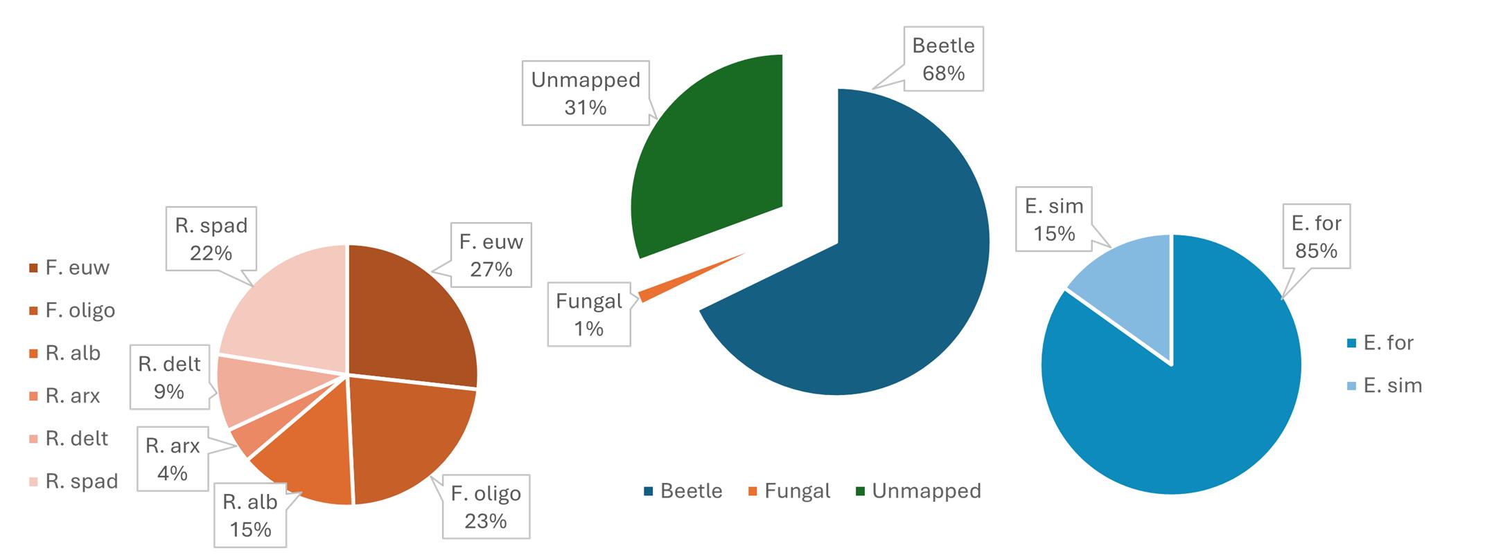
Figure 11. Percent of transcripts mapped to each genome in Euwallacea–Fusarium (BH) samples. The center pie chart shows the mapping of all transcripts. Fungal and beetle species breakdown is shown on the left and right, respectively. Data represent averages of five BH samples.
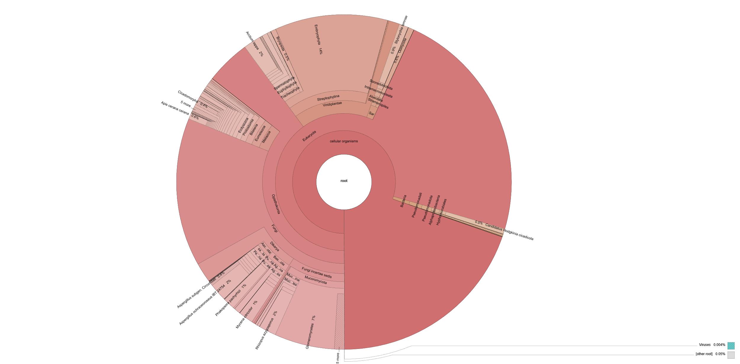
Figure 12. Krona plot of cicada–Massospora (C) sample unmapped transcripts. An interactive version of this plot can be found in the Supplemental Information section.
Figure 11 explores symbionts present in Euwallacea–Fusarium BH samples and addresses troubleshooting when lacking a reference genome. While Fusarium is the primary nutritional symbiont, other fungal interlopers are known to be present. To further explore the mycangial microbial community, additional genomes were used as references. Four Raffaelea and two Fusarium genomes were added to BBSplit, and the resulting proportion of transcripts for each species can be seen in the leftmost pie chart of Figure 11. Transcript counts used to create Figures 10 and 11 can be found in Supplementary Information Dataset S1. In BH samples, coverage was strong enough to pick up difficult-to-culture symbionts within the mycangia. Table 2 shows that, on average, 36.5% of F. oligoseptatum genes are detected when mapping transcripts. This demonstrates that the mapping depth of the partner of interest allows downstream analysis. The genome of Fusarium oligoseptatum has 17,904 genes and 17,740 protein-coding genes. Across the 5 BH samples, an average of 36.5% of genes were detected from expressed mRNA. Only genes with a TPM value above 5 were considered for this analysis. Not all genes are constitutively expressed and thus expected to be detected. F. oligoseptatum mRNA accounted for 23% of detected fungal transcripts, while fungal transcripts represent only 1% of total mRNA detected. The rate of gene detection shows that the small proportion of F. oligoseptatum transcripts present still allows for downstream analysis. E. validus is the expected host species, but it lacks a published genome. Rather than de novo assembly, published genomes of the two most closely related species to E. validus were chosen as reference genomes. E. fornicatus is most closely related to E. validus, resulting in 85% of E. validus transcript mapping to E. fornicatus. The 15% of beetle transcripts mapped to E. similis would not have been captured if only the E. fornicatus genome had been used because of poor mapping scores. These results are represented graphically in the rightmost pie chart in Figure 11.
Unmapped reads can be explained by poor sequence quality, novel transcripts and splice junctions, contamination/eRNA, sequencing errors, and mutations, which may be more prevalent in quickly evolving genes. To further investigate this, Krona plots of unmapped reads were created. Figure 12 shows unmapped C sample transcripts. 12% of these transcripts remain unclassified, 0.004% resemble viral RNA, and 70% resemble eukaryotic RNA. The Krona plot revealed plant transcripts in C samples. These transcripts could be from feeding prior to infection or from contact throughout the flight. Krona plots are interactive, and a link to a plot exploring C unmapped transcripts can be found in Supplemental Information Dataset S2. Together, this section aims to validate that RNA extraction, RNA sequencing, and data analysis were successful using the above protocol.
Table 2. Gene-level coverage for F. oligoseptatum reads
| Sample | Input reads | Genes in F. oligo | Genes mapped | Genes mapped (%) |
| BH1 | 355,406 | 17,904 | 6,430 | 35.9 |
| BH2 | 729,752 | 17,904 | 7,512 | 42.0 |
| BH3 | 448,664 | 17,904 | 7,159 | 40.0 |
| BH4 | 413,306 | 17,904 | 5,360 | 29.9 |
| BH5 | 527,540 | 17,904 | 6,174 | 34.5 |
General notes and troubleshooting
General notes
1. To increase RNA quality, consider adding a second ethanol wash or additional chloroform treatment and/or re-doing RNA extraction by combining the RNA sample with 1 mL of TRIzol and continuing from step B12.
2. When centrifuging to produce a pellet and during cleaning steps, it is important to know where the pellet should be, so that if it is not seen, you can avoid pipetting it up. To this end, microcentrifuge tubes are always angled so that the point on the cap is facing inward during centrifugation. The side of the tube facing outward will contain the pellet; pipetting out from the inward side will reduce loss of product (Figure 13).
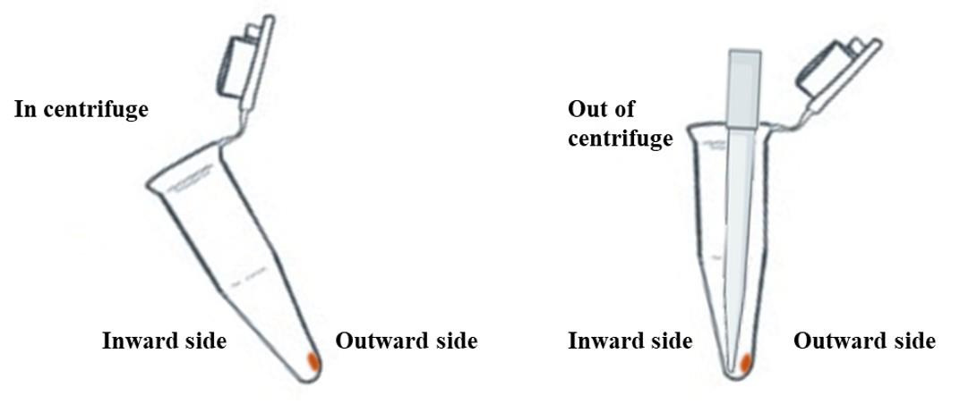
Figure 13. Diagram showing how to avoid the RNA pellet when removing the supernatant during cleaning steps. The orange dot represents the pellet, which will be white when visible. The RNA pellet will form at the outward side of the tube during centrifugation. Take up the supernatant from the inward side to avoid removing any RNA.
3. Each centrifugation step has a time ending in 30 s, rather than a whole number, to account for the time it takes the centrifuge to reach speed. This timing may differ by machine or setup (slow vs. fast acceleration); consider changing it to match how long your centrifuge takes to reach speed.
Troubleshooting
Problem 1: Low concentration.
Possible causes: Not enough aqueous phase taken, too little sample, too much water added, or quality of grinding.
Solutions: Take more aqueous phase, start with more sample.
Problem 2: Poor 260/280 Nanodrop value.
Possible cause: Interphase was disturbed and taken up.
Solution: Keep the pipette tip as high in the aqueous phase as possible, pull up slowly, and dispense in aliquots of 100 μL so that you can stop and discard if any white precipitate is aspirated into the tip.
Supplementary information
The following supporting information can be downloaded here:
1. Dataset S1. Transcript mapping table
2. Dataset S2. Link to Karona plot
Acknowledgments
Conceptualization, Writing—original draft, Investigation, M.L.; Review and Editing, E.S., M.K., T.K.; Validation, Data analysis, J.E.S.; Supervision, M.K., T.K.; Funding acquisition, M.L., M.K. This work was made possible by funding from the Paul G. Moe Memorial Endowment Award. We would like to acknowledge the WVU Genomics Core Facility, Morgantown, WV, for support provided to help make this publication possible, and CTSI Grant #U54 GM104942, which provides financial support to the Core Facility. Computational resources were provided by the WVU Research Computing Thorny Flat HPC cluster, partly funded by NSF OAC-1726534. J.E.S is a CIFAR Fellow in the program Fungal Kingdom: Threats and Opportunities and was supported by NSF EF-2125066. The following figures were created using BioRender: Graphical overview, https://BioRender.com/b0qhywl; Protocol Workflow, BioRender.com/b0qhywl
Competing interests
No conflict of interest is declared regarding this article.
References
- Baskett, C. A. and Schemske, D. W. (2015). Mutualism, Chapter 5: Evolution and Genetics of Mutualism. Oxford University Press. 77–92. https://doi.org/10.1093/acprof:oso/9780199675654.003.0005
- Mueller, U. G., Gerardo, N. M., Aanen, D. K., Six, D. L. and Schultz, T. R. (2005). The Evolution of Agriculture in Insects. Annu Rev Ecol Evol Syst. 36(1): 563–595. https://doi.org/10.1146/annurev.ecolsys.36.102003.152626
- Lovett, B., Macias, A., Stajich, J. E., Cooley, J., Eilenberg, J., de Fine Licht, H. H. and Kasson, M. T. (2020). Behavioral betrayal: How select fungal parasites enlist living insects to do their bidding. PLoS Pathog. 16(6): e1008598. https://doi.org/10.1371/journal.ppat.1008598
- Ankeny, R. A. and Leonelli, S. (2011). What’s so special about model organisms? Stud Hist Philos Sci Part A. 42(2): 313–323. https://doi.org/10.1016/j.shpsa.2010.11.039
- Abzhanov, A., Extavour, C. G., Groover, A., Hodges, S. A., Hoekstra, H. E., Kramer, E. M. and Monteiro, A. (2008). Are we there yet? Tracking the development of new model systems. Trends Genet. 24(7): 353–360. https://doi.org/10.1016/j.tig.2008.04.002
- Spahr, E., Kasson, M. T. and Kijimoto, T. (2020). Micro-computed tomography permits enhanced visualization of mycangia across development and between sexes in Euwallacea ambrosia beetles. PLoS One. 15(9): e0236653. https://doi.org/10.1371/journal.pone.0236653
- Joseph, R. and Keyhani, N. O. (2021). Fungal mutualisms and pathosystems: life and death in the ambrosia beetle mycangia. Appl Microbiol Biotechnol. 105(9): 3393–3410. https://doi.org/10.1007/s00253-021-11268-0
- Cooley, J. R., Marshall, D. C. and Hill, K. B. R. (2018). A specialized fungal parasite (Massospora cicadina) hijacks the sexual signals of periodical cicadas (Hemiptera: Cicadidae: Magicicada). Sci Rep. 8(1): 1432. https://doi.org/10.1038/s41598-018-19813-0
- Macias, A. M., Geiser, D. M., Stajich, J. E., Łukasik, P., Veloso, C., Bublitz, D. C., Berger, M. C., Boyce, G. R., Hodge, K., Kasson, M. T., et al. (2020). Evolutionary relationships among Massospora spp. (Entomophthorales), obligate pathogens of cicadas. Mycologia. 112(6): 1060–1074. https://doi.org/10.1080/00275514.2020.1742033
- Anderson, J. A., Corbin, E. M., Lovett, B., Kasson, M. T. and LaDouceur, E. E. B. (2023). Histologic findings of Massospora cicadina infection in periodical cicadas (Magicicada septendecim). Vet Pathol. 60(5): 704–708. https://doi.org/10.1177/03009858231156790
- Di Tommaso, P., Chatzou, M., Floden, E. W., Barja, P. P., Palumbo, E. and Notredame, C. (2017). Nextflow enables reproducible computational workflows. Nat Biotechnol. 35(4): 316–319. https://doi.org/10.1038/nbt.3820
- Ewels, P., Peltzer, A., Fillinger, S., Patel, H., Alneberg, J., Wilm, A., Garcia, M. U., Paolo Di Tommaso and Nahnsen, S. (2020). The nf-core framework for community-curated bioinformatics pipelines, mc-core.rnaseq v3.22.2. 10.1038/s41587-020-0439-x version 10.5281/zenodo.1400710
Article Information
Publication history
Received: Mar 25, 2026
Accepted: May 22, 2026
Available online: Jun 22, 2026
Published: Jul 5, 2026
Copyright
© 2026 The Author(s); This is an open access article under the CC BY-NC license (https://creativecommons.org/licenses/by-nc/4.0/).
How to cite
Laws, M., Burns, E. S., Kasson, M. T., Kijimoto, T. and Stajich, J. E. (2026). Simultaneous Transcriptomic Analysis of Both Host and Symbiont in Insect–Fungus Interactions. Bio-protocol 16(13): e5739. DOI: 10.21769/BioProtoc.5739.

 Download Citation in RIS Format
Category
Bioinformatics and Computational Biology
Molecular Biology > RNA > RNA extraction
Systems Biology > Transcriptomics > RNA-seq
Do you have any questions about this protocol?
Post your question to gather feedback from the community. We will also invite the authors of this article to respond.
 Post a Question


