


- Protocols

- Articles and Issues
- For Authors
- About
- Become a Reviewer


Stepwise Protocol for Alternative Splicing Analysis in Single-Cell SMART-Seq2 RNA-Seq Data

Published: Vol 16, Iss 12, Jun 20, 2026 DOI: 10.21769/BioProtoc.5735 Views: 477
Reviewed by: Anonymous reviewer(s)
 PDF
PDF  Ask a question
Original research article
The authors used this protocol in:

Dec 2025
Advertisement


Protocol Collections
Comprehensive collections of detailed, peer-reviewed protocols focusing on specific topics






Abstract
RNA alternative splicing (AS) is an essential process that expands transcriptomic and proteomic diversity in eukaryotic cells and contributes to cellular heterogeneity across physiological and pathological conditions in humans. With the advent of single-cell RNA sequencing (scRNA-seq), it has become possible to study AS at cellular resolution, although robust and standardized analytical workflows remain to be developed. Here, we present a stepwise protocol for analyzing AS in single cells from pediatric high-grade gliomas (pHGGs) harboring the histone H3.3 lysine 27-to-methionine (H3.3K27M) mutation using SMART-Seq2 scRNA-seq data. Starting from raw sequencing reads, the workflow includes read alignment, gene-level quantification, splice junction and intron quantification, and single-nucleotide variant-based mutation detection. Gene expression–based clustering and cell-type annotation are performed by using the Seurat R package. AS analysis in tumor cells is then conducted using the MARVEL R package in combination with customized scripts to calculate percent spliced-in (PSI) values, identify variable AS events, perform dimensionality reduction, cluster cells, conduct differential AS analysis, and visualize splicing patterns. This protocol provides a reproducible and comprehensive framework for dissecting AS dynamics at single-cell resolution. It is readily adaptable to other SMART-Seq2 datasets and facilitates systematic investigation of splicing heterogeneity in diverse biological contexts.
Key features
• Protocol for single-cell RNA alternative splicing (AS) analysis in pediatric high-grade gliomas (pHGGs) with H3.3K27M mutation using SMART-Seq2 data.
• Integrates gene expression–based clustering and genetic mutation to identify tumor populations.
• MARVEL plus custom scripts enable PSI computation, variable AS detection, clustering, differential splicing analysis, and visualization of splicing patterns.
• Flexible workflow applicable to other full-length scRNA-seq datasets for studying AS dynamics in cancer and development.
Keywords: Single-cell RNA sequencing Alternative splicing
Pediatric high-grade glioma
H3.3K27M mutation
SMART-Seq2
MARVEL
Alternative splicing
Pediatric high-grade glioma
H3.3K27M mutation
SMART-Seq2
MARVEL
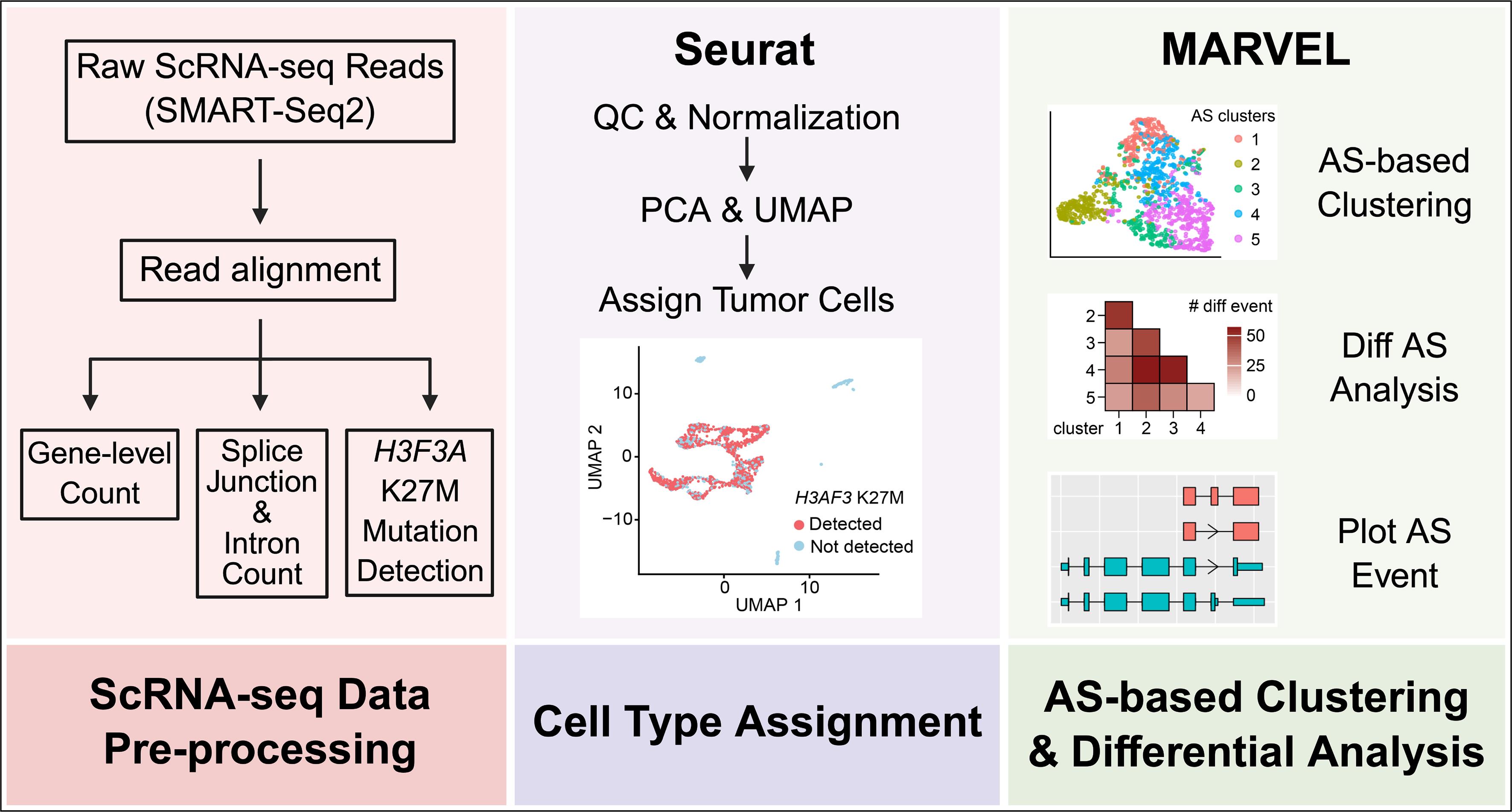
Graphical overview
Background
RNA alternative splicing (AS) is a fundamental regulatory mechanism in eukaryotic cells that expands transcriptomic and proteomic diversity by generating multiple RNA transcripts and protein isoforms from a single gene through differential exon usage [1]. This process plays critical roles in cell fate specification, tissue development, and the regulation of cellular states, and its dysregulation has been implicated in numerous diseases, including neurological disorders and cancer [2,3]. Understanding AS at single-cell resolution is therefore essential for dissecting cellular heterogeneity and dynamic state transitions in complex biological systems.
Advances in single-cell RNA sequencing (scRNA-seq) technologies have enabled transcriptome-wide profiling of individual cells; however, most widely used platforms, such as droplet-based methods [4,5], are limited in their ability to accurately quantify full-length transcripts and splice isoforms. Full-length scRNA-seq protocols such as SMART-Seq2 [6] enable accurate detection of splice junctions and isoform usage, providing a strong foundation for AS analysis at single-cell resolution [7]. Computational tools such as MARVEL [8] facilitate quantification and downstream analysis of splicing events, including calculation of percent spliced-in (PSI) values, differential AS analysis, and dimensionality reduction methods such as principal component analysis (PCA) and uniform manifold approximation and projection (UMAP). While MARVEL provides a robust framework for AS quantification in single-cell RNA-seq data, it has relatively limited built-in support for further downstream analyses, such as filtering AS events, clustering cells using AS features, and visualization of specific AS events. As a result, constructing a reproducible, end-to-end workflow from raw sequencing data to integrated biological interpretation remains challenging.
This protocol provides a comprehensive and stepwise workflow for analyzing AS using SMART-Seq2 scRNA-seq data, integrating gene expression and splicing analyses within a unified framework. Starting from raw sequencing reads, the pipeline includes read alignment, gene and splice junction quantification, mutation detection, and gene expression–based clustering and annotation. AS analysis is then performed using MARVEL in combination with customized steps to calculate PSI values, identify variable AS events, perform dimensionality reduction, cluster cells based on AS features, and conduct differential splicing analysis. This workflow emphasizes reproducibility, flexibility, and compatibility with standard single-cell analysis pipelines.
While this protocol is demonstrated in the context of pediatric high-grade glioma (pHGG) with H3.3K27M mutation, it is broadly applicable to other biological systems where full-length scRNA-seq data are available. It can be adapted to study AS dynamics in normal development, disease progression, and treatment response, and may be extended to investigate splicing regulation, isoform-specific functions, and interactions with genetic or epigenetic alterations.
Equipment
A personal computer or access to a high-performance computing (HPC) cluster is required.
Software and datasets
1. Raw FASTQ files of H3.3K27M glioma scRNA-seq dataset (https://duos.broadinstitute.org/dataset/DUOS-000107), free, application required for access
2. Codes, processed data, and analysis outputs from this protocol (https://zenodo.org/records/20213707), v2, free
3. STAR (https://github.com/alexdobin/STAR?tab=readme-ov-file), 2.7.9a, free
4. Samtools (https://www.htslib.org/), 1.6, free
5. HTSeq-count (https://htseq.readthedocs.io/en/latest/htseqcount.html), 2.0.9, free
6. Bedtools (https://bedtools.readthedocs.io/en/latest/), 2.30.0, free
7. RSEM (https://github.com/deweylab/RSEM), 1.3.3, free
8. Monovar (https://github.com/KChen-lab/MonoVar, python 2 required), NA, free
9. Python (https://www.python.org/), 2.7.5, free
10. R (https://www.r-project.org/), 4.4.0, free
11. R package Seurat (https://satijalab.org/seurat/), 5.4.0, free
12. R package MARVEL (https://github.com/wenweixiong/MARVEL), 2.0.5, free
13. R package dplyr (https://dplyr.tidyverse.org/), 1.2.0, free
14. R package kernlab (https://github.com/cran/kernlab), 0.9-33, free
15. R package tidyverse (https://tidyverse.org/packages/), 2.0.0, free
16. R package ggplot2 (https://ggplot2.tidyverse.org/), 4.0.2, free
17. R package patchwork (https://patchwork.data-imaginist.com/), 1.3.2, free
18. R package ggtranscript (https://github.com/dzhang32/ggtranscript), 1.0.0, free
19. R package gghalves (https://github.com/erocoar/gghalves), 0.1.4, free
Procedure
This protocol describes a workflow for processing single-cell SMART-seq RNA-seq data from raw reads to gene expression–based clustering and alternative splicing analysis. An overview of the analysis pipeline is shown in Figure 1.
A. Single-cell RNA-seq data preprocessing
This section describes the preprocessing workflow for scRNA-seq data generated using SMART-Seq2 or other plate-based protocols. The workflow includes acquisition of raw FASTQ files, alignment of reads to the reference genome, gene-level quantification, and detection of splice junctions and retained introns. An optional single-nucleotide variant (SNV) analysis step is included for the demonstration dataset used in this protocol to determine H3F3A K27M mutation status, which was used together with transcriptome-based clustering to distinguish tumor and non-tumor cells, as H3F3A is highly expressed and detectable by scRNA-seq in H3K27M glioma. This step can be modified or omitted depending on the biological system and study design. Example code is provided for each step, and the complete code for this section is available in Code S1.
1. Acquisition of scRNA-seq data
This protocol requires raw FASTQ sequencing data generated from scRNA-seq experiments using the SMART-Seq2 or other plate-based protocols that provide full transcript coverage across mRNA molecules. For the example analysis presented in this protocol, the pHGG H3.3K27M scRNA-seq data was obtained from the previously published dataset by Mariella G. Filbin et al. via the Data Use Oversight System (DUOS) data library [9].
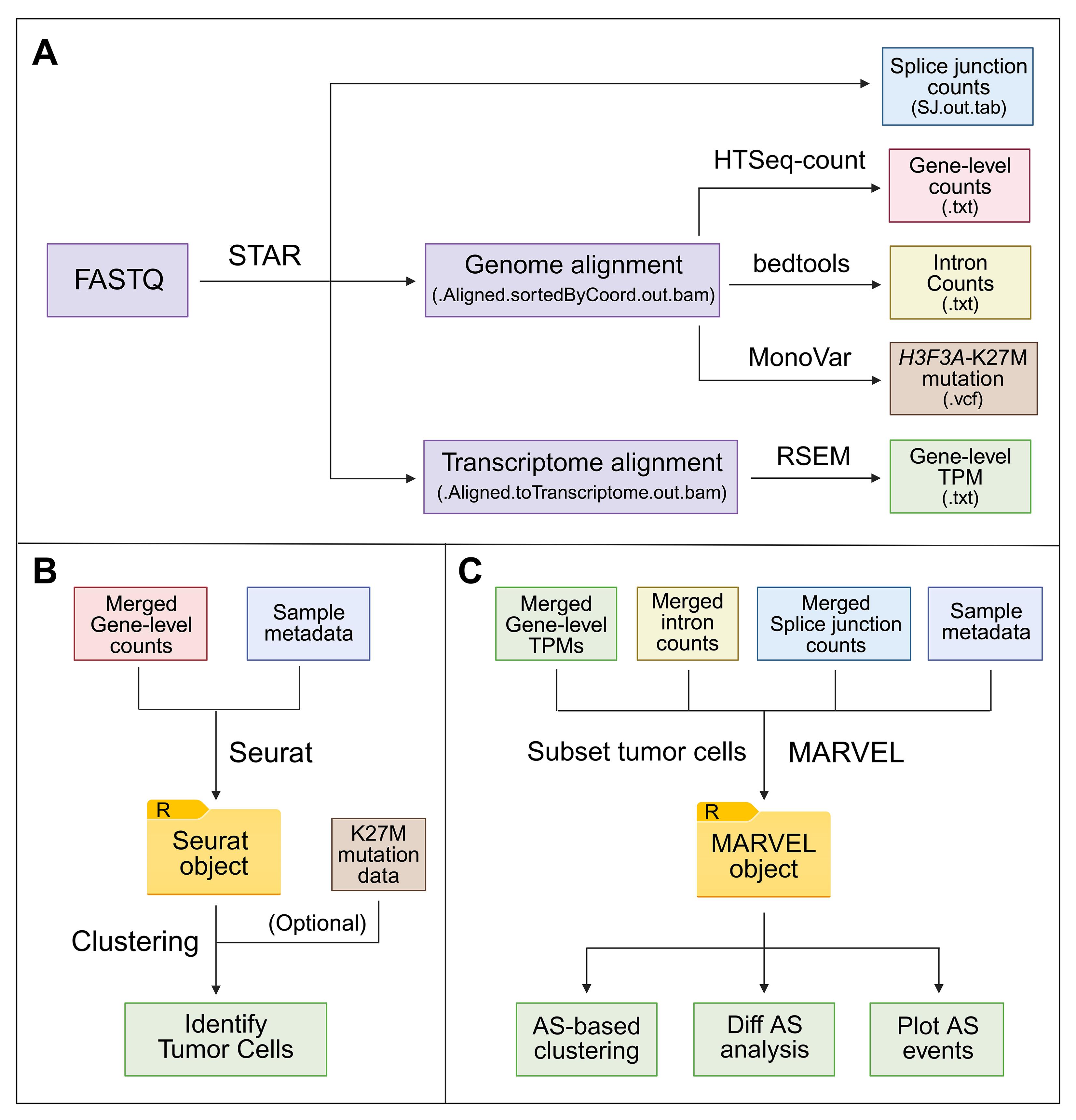
Figure 1. Overview of the SMART-Seq2 scRNA-seq alternative splicing analysis workflow. Workflow diagram showing the major steps for gene expression and alternative splicing (AS) analysis of SMART-Seq2 scRNA-seq data, including read alignment, quantification, optional mutation analysis, cell clustering and annotation, percent spliced-in (PSI) quantification with MARVEL, AS-based analyses, and downstream visualization. Input/output file types and software tools used at each step are indicated throughout the workflow.
2. Alignment of scRNA-seq reads to the reference genome and quantification of splice junction reads
Align the raw FASTQ reads to the GRCh38 human reference genome using the STAR aligner (v2.7.9a) [10] with genome files from GENCODE Release 44 (GRCh38.p14). At the same time, STAR reports splice junction information during alignment in the output file SJ.out.tab, which contains genomic coordinates and read counts supporting each splice junction. Merge the splice junction counts from all samples in R to generate a splice junction count matrix for downstream AS analysis in MARVEL.
Note: The example data are paired-end reads. If using single-end data, modify the script according to the STAR documentation.
STAR --runThreadN 10 \--genomeDir ~/Genome/STAR/GRCh38 \--readFilesCommand zcat \--readFilesIn ${fastq} \--outFileNamePrefix STAR/${sample}. \--outSAMtype BAM SortedByCoordinate3. Gene-level quantification
Quantify gene-level read counts using HTSeq-count (v2.0.9) [11] with the GENCODE Release 44 (GRCh38.p14) annotation. Merge the resulting count files from all samples in R (v4.4.0) to generate a gene expression count matrix for downstream gene-level expression analyses in Seurat.
htseq-count -f bam STAR/${sample}.Aligned.sortedByCoord.out.bam \${gtf} -s no > HTSeq/${sample}.txt4. Quantification of retained intron reads
Calculate read coverage across all intron regions for each sample using Bedtools (v2.30.0) [12] and Samtools (v1.6) [13]. Merge the resulting intron counts from all samples in R to generate a retained intron count matrix for downstream AS analysis in MARVEL.
bedtools coverage \-g GRCh38.primary_assembly.genome.bed \-split \-sorted \-d \-a MARVEL/RI_Coordinates.bed \-b STAR/${sample}.Aligned.sortedByCoord.out.bam \> RI_Counts/${sample}.txt5. Gene-level transcripts per million (TPM) quantification
Calculate gene-level transcript abundance in TPM using RSEM (v1.3.3) [14]. RSEM estimates gene and transcript expression levels from alignment files mapped to the transcriptome. Use the BAM files generated from STAR alignment as input. The resulting output files contain both gene-level TPM values, which can be used for downstream analysis in MARVEL.
rsem-calculate-expression --bam \--paired-end \-p 1 \STAR/${sample}.Aligned.toTranscriptome.out.bam \~/Genome/RSEM/GRCh38.primary_assembly.refseq \RSEM/${sample}6. (Optional) Single-cell SNV analysis of H3F3A K27M mutation
Determine the H3F3A K27M mutation status in individual cells using SNV analysis. Process reads with Samtools (v1.6) to generate pileup information restricted to the H3F3A locus and perform variant calling with MonoVar [15]. Use the resulting VCF file to assess the presence or absence of the K27M mutation in each cell based on read support and allele frequency. Integrate mutation status with gene expression data for downstream clustering and cell-type annotation in Seurat.
samtools mpileup -BQ0 -d 10000 -f ${genome_fa} -q 40 -l SNV/H3K27M.bed -b SNV/input_list.txt | python MonoVar-master/src/monovar.py -p 0.002 -a 0.2 -t 0.05 -m 20 -f ${genome_fa} -b SNV/input_list.txt -o SNV/monovar_output.vcfB. Gene expression–based clustering and cell-type assignment
In this section, single-cell gene expression data are processed to identify transcriptionally distinct cell populations and annotate cell types using the R package Seurat (v5.4.0) [16]. Starting from the gene-level count matrix, cells are filtered for quality, clustered based on gene expression patterns, and visualized in UMAP two dimensions. Tumor cell populations are identified using canonical marker genes for each cell type, together with H3F3A K27M mutation status, and are prepared for downstream AS analysis. Example code is provided for each step, and the complete code for this section is available in Code S2. The Seurat object generated from this analysis is available on Zenodo (https://zenodo.org/records/20213707).
1. Load the gene-level count matrix generated by HTSeq-count and the associated metadata into Seurat (v5.4.0). Include the H3F3A K27M mutation status in the metadata for each cell.
seu_K27M <- CreateSeuratObject(counts = count_data, project = “K27M”)2. Filter cells based on quality control metrics, including total read counts, number of detected genes, and mitochondrial read fraction.
Note: The parameter settings for cell filtration should be optimized for each dataset.
seu_K27M[[“percent.mt”]] <- PercentageFeatureSet(seu_K27M, pattern = “^MT-”)seu_filt_K27M <- subset(seu_K27M, subset =nFeature_RNA > 1000 &nFeature_RNA < 15000 &nCount_RNA < 4000000 &percent.mt < 20)3. Normalize and scale the filtered data to correct for technical variability across cells.
seu_filt_K27M <- NormalizeData(seu_filt_K27M, normalization.method = “LogNormalize”, scale.factor = 10000)seu_filt_K27M <- ScaleData(seu_filt_K27M, features = rownames(seu_filt_K27M))4. Identify highly variable genes for dimensionality reduction.
seu_filt_K27M <- FindVariableFeatures(seu_filt_K27M, selection.method = “vst”, nfeatures = 2000)5. Perform principal component analysis (PCA) using the selected variable genes and determine the number of significant principal components using an elbow plot.
seu_filt_K27M <- RunPCA(seu_filt_K27M, features = VariableFeatures(object = seu_filt_K27M))ElbowPlot(seu_filt_K27M)6. Construct a shared nearest neighbor (SNN) graph and perform graph-based clustering to identify transcriptionally distinct cell populations.
Note: The number of dimensions used in FindNeighbors and the resolution parameter in FindClusters should be optimized for each dataset.
seu_filt_K27M <- FindNeighbors(seu_filt_K27M, dims = 1:20)seu_filt_K27M <- FindClusters(seu_filt_K27M, resolution = 1.2)7. Visualize clusters in two dimensions using uniform manifold approximation and projection (UMAP) (Figure 2A).
seu_filt_K27M <- RunUMAP(seu_filt_K27M, dims = 1:20)DimPlot(seu_filt_K27M, reduction = “umap”, label = TRUE, group.by = “seurat_clusters”, pt.size = 0.1) + NoLegend()8. Annotate cell types using canonical marker gene expression—including SOX2 for pHGG tumor cells, PTPRC/CD45 for hematopoietic cells, CD14 for myeloid cells, CD3E for T cells, CSF3R for neutrophils, and MBP for oligodendrocytes—together with H3F3A K27M mutation status to define tumor cell populations (Figure 2B, C). Cells assigned to Seurat clusters other than 10, 12, and 13, and harboring the H3F3A K27M mutation, were classified as tumor cells for downstream AS analysis.
Note: In this example, tumor and non-tumor cells are distinguished using transcriptome-based clustering together with H3F3A K27M mutation status, since H3F3A is highly expressed and detectable by scRNA-seq. In tumor types with lower mutation expression, alternative strategies such as copy number variation (CNV) analysis can be used to identify tumor cells, for example, with tools like copyKAT [17] or SCEVAN [18].
DimPlot(seu_filt_K27M, reduction = “umap”, pt.size = 0.1, group.by = “SNV_K27M”, cols = c(“Mut” = “#f36569”, “Non-mut” = “#a2d2e7”))FeaturePlot(seu_filt_K27M, features = c(“SOX2”, “PTPRC”, “CD14”, “CD3E”, “CSF3R”, “MBP”), ncol = 3, cols = c(“grey”,”red”), pt.size = 0.5)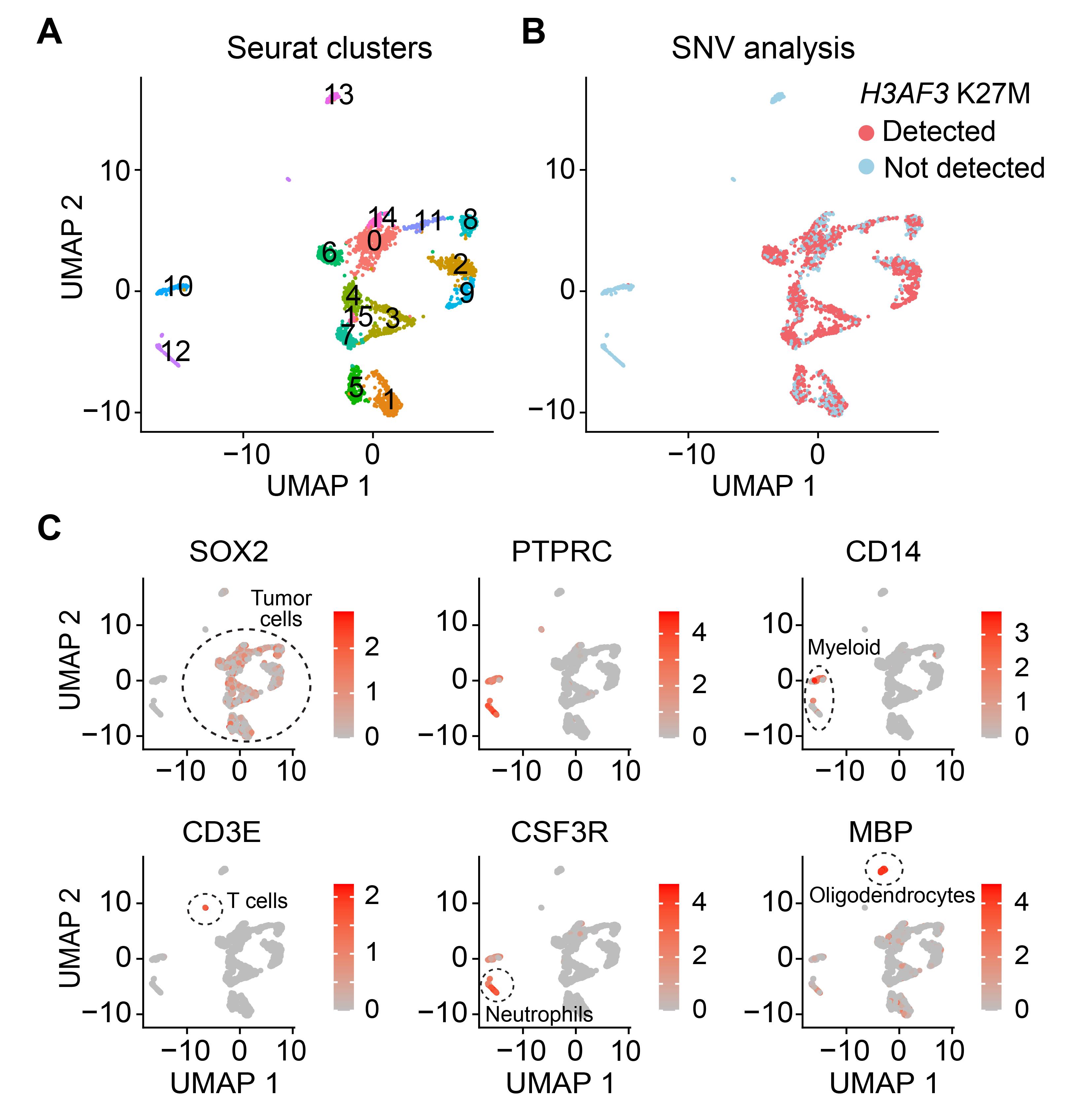
Figure 2. Gene expression–based clustering and cell-type annotation of pHGG H3.3K27M scRNA-seq data. (A) UMAP of cells colored by Seurat cluster identity. (B) UMAP of cells colored by H3.3K27M mutation status. (C) Feature plots showing expression of canonical marker genes used for cell-type annotation.
C. AS-based clustering and differential AS analysis
This section describes the workflow for AS-based clustering and differential AS analysis in pHGG H3.3K27M tumor cells using MARVEL (v2.0.5) [8] and customized scripts. Tumor cells identified from gene-level Seurat analysis are used to construct a MARVEL object, compute PSI values for multiple AS event types, and select variable AS events for dimensionality reduction. PCA and UMAP, followed by K-means and spectral clustering, are applied to identify AS-based clusters. Pairwise comparisons between clusters identify differentially spliced events, and PSI distributions of specific AS events are visualized to interpret AS patterns. Steps C1, C2, C4, and C6 are performed using the functions from the MARVEL R package, while steps C3, C5, and C7 are implemented via customized scripts to supplement the MARVEL analysis. Example code is provided for each step, and the complete code for this section is available in Code S3. The MARVEL object and other analysis outputs from this section are available on Zenodo (https://zenodo.org/records/20213707).
1. Create MARVEL object
Initialize the MARVEL object with sample metadata, splicing features, gene features, gene transfer format (GTF) annotation, splice junction counts, retained intron counts, and gene expression data. The formats for sample metadata, splicing features, gene features, and GTF annotation should follow the MARVEL guidelines (https://wenweixiong.github.io/ MARVEL_Plate.html). Splice junction counts, retained intron counts, and gene expression TPM data are generated as described in steps A2, A4, and A5.
marvel <- CreateMarvelObject(SplicePheno = sample_metadata,SpliceFeature = df.feature.list,GeneFeature = gene_metadata,GTF = gtf,SpliceJunction = sj_count,IntronCounts = RI_count,Exp = df.tpm)2. Compute PSI for each type of AS event
Detect alternative first exon (AFE) and alternative last exon (ALE) events. Filter cryptic alternative 5′ splice site (A5SS)/alternative 3′ splice site (A3SS) events and remove cryptic splice sites for AFE/ALE. Compute PSI values for skipped exon (SE), mutually exclusive exon (MXE), retained intron (RI), A5SS, A3SS, AFE, and ALE events using coverage thresholds and quality filters.
Note: The parameter settings for min.cells, min.expr, CoverageThreshold, and UnevenCoverageMultiplier should be optimized for each dataset to ensure accurate detection and quantification of AS events. Depending on sequencing depth, cell number, and data quality, adjusting these parameters may improve PSI estimation and reduce missing values.
# Detect AFEmarvel <- DetectEvents(MarvelObject=marvel,min.cells=20,min.expr=1,track.progress=TRUE,EventType=“AFE”)# Detect ALEmarvel <- DetectEvents(MarvelObject=marvel,min.cells=20,min.expr=1,track.progress=TRUE,EventType=“ALE”)# filtering in of cryptic A5SS and A3SSmarvel <- SubsetCrypticSS(marvel, DistanceToCanonical = 100, EventType=“A5SS”)marvel <- SubsetCrypticSS(marvel, DistanceToCanonical = 100, EventType=“A3SS”)# filtering out of cryptic A5SS and A3SS for the list of AFE and ALEmarvel <- RemoveCrypticSS(marvel, DistanceToCanonical = 100, EventType=“AFE”)marvel <- RemoveCrypticSS(marvel, DistanceToCanonical = 100, EventType=“ALE”)# Check splicing junction datamarvel <- CheckAlignment(MarvelObject=marvel, level=“SJ”)# Validate, filter, compute SE splicing eventsmarvel <- ComputePSI(MarvelObject=marvel,CoverageThreshold=10,UnevenCoverageMultiplier=10,EventType=“SE”)# Validate, filter, compute MXE splicing eventsmarvel <- ComputePSI(MarvelObject=marvel,CoverageThreshold=10,UnevenCoverageMultiplier=10,EventType=“MXE”)# Validate, filter, compute RI splicing eventsmarvel <- ComputePSI(MarvelObject=marvel,CoverageThreshold=10,EventType=“RI”,thread=4)# Validate, filter, compute A5SS splicing eventsmarvel <- ComputePSI(MarvelObject=marvel,CoverageThreshold=10,EventType=“A5SS”)# Validate, filter, compute A3SS splicing eventsmarvel <- ComputePSI(MarvelObject=marvel,CoverageThreshold=10,EventType=“A3SS”)# Validate, filter, compute AFE splicing eventsmarvel <- ComputePSI(MarvelObject=marvel,CoverageThreshold=10,EventType=“AFE”)# Validate, filter, compute ALE splicing eventsmarvel <- ComputePSI(MarvelObject=marvel,CoverageThreshold=10,EventType=“ALE”)3. Identify AS events with variable PSI values across tumor cells for downstream dimensionality reduction
To focus on informative AS events, variability metrics are computed. For each AS event, the standard deviation of PSI values across tumor cells and the number and proportion of cells with detected PSI are calculated. Events are then filtered to retain only those with sufficient variability and data coverage. In this example, events with a standard deviation of PSI greater than 0.1 and non-missing values in more than 5% of cells are selected for downstream dimensionality reduction (Figure 3A).
Note: The thresholds for PSI standard deviation (sd_cutoff) and event coverage (nonNA_percent_cutoff) should be adjusted per dataset, as they may affect AS-based clustering outcomes.
# Define AS event typesAS_types <- c(“SE”, “MXE”, “RI”, “A5SS”, “A3SS”, “AFE”, “ALE”)# Initialize listPSI_variability <- list()# Compute variability metrics for each AS typefor (event in AS_types) {df <- PSI[[event]]metrics <- data.frame(sd = apply(df[, -1], 1, function(x) sd(x, na.rm = TRUE)),non_NA = apply(df[, -1], 1, function(x) sum(!is.na(x))),row.names = df$tran_id)metrics$type <- eventPSI_variability[[event]] <- metrics}# Merge all AS types into a single data framePSI_variability_merge <- do.call(rbind, PSI_variability)PSI_variability_merge <- na.omit(PSI_variability_merge)# Compute percent of non-NA valuesPSI_variability_merge$non_NA_percent <- PSI_variability_merge$non_NA / nrow(marvel[[“SplicePheno”]])# Set cut-off for variable eventssd_cutoff <- 0.1nonNA_percent_cutoff <- 0.05event_var <- rownames(PSI_variability_merge)[PSI_variability_merge$sd > sd_cutoff & PSI_variability_merge$non_NA_percent > nonNA_percent_cutoff]4. PCA analysis and UMAP visualization
Perform PCA based on the PSI values of variable AS events and visualize clusters using UMAP. Bayesian imputation is applied to account for missing values [19], and elbow plots are used to determine the number of principal components for dimensionality reduction (Figure 3B). The resulting PCA coordinates are then used to generate two-dimensional UMAP embeddings for visualizing AS-based cell clusters.
Notes:
1. MARVEL implements a Bayesian-based imputation approach for PSI values (method.impute = “Bayesian”), which is recommended for handling sparsity in single-cell splicing data. Alternative imputation methods (e.g., kNN, MAGIC, ALRA) can be applied using other packages.
2. Parameters for PCA (e.g., number of principal components) and UMAP should be optimized for each dataset.
3. Setting a fixed seed.umap is recommended to ensure reproducibility of UMAP embeddings.
# Compute PSI.Posterior for Bayesian imputation in PCA analysis.marvel <- ComputePSI.Posterior(marvel)# elbow plotmarvel <- RunPCA(MarvelObject = marvel,features = event_var,cell.group.column = “seurat_clusters”,point.size = 1,level = “splicing”,method.impute = “Bayesian”,mode = “elbow.plot”,npc.elbow.plot = 20)# PCAnpc.umap <- 10marvel <- RunPCA(MarvelObject = marvel,features = event_var,cell.group.column = “seurat_clusters”,point.size = 1,point.stroke = 0,level = “splicing”,method.impute = “Bayesian”,mode = “pca”,npc.umap = npc.umap)# UMAPmarvel <- RunPCA(MarvelObject = marvel,features = event_var,cell.group.column = “seurat_clusters”,point.size = 1,point.stroke = 0,level = “splicing”,method.impute = “Bayesian”,mode = “umap”,seed.umap = 42,npc.umap = npc.umap)5. Identify AS-based tumor cell clusters
Use PCA and UMAP data from the MARVEL object to identify AS-based tumor cell clusters. Select the top principal components for clustering and apply both K-means [20] and spectral clustering [21] to define AS-based cell clusters. Visualize the clustering results on the UMAP embedding to evaluate concordance between methods (Figure 3C). Map the expression of specific neural lineage marker genes—including OLIG1 and PDGFRA for oligodendrocyte precursor cells (OPCs), CD24 for neural progenitor cells (NPCs), PLP1 for oligodendrocytes, and AQP4 for astrocytes—onto the AS-based UMAP to interpret the relationship between lineage identity and AS clusters (Figure 3D).
Notes:
1. The number of principal components used for clustering and the number of clusters (k) should be optimized for each dataset, as these parameters can influence AS-based cluster identification.
2. Different clustering methods (e.g., K-means and spectral clustering) may yield varying results; comparing multiple approaches is recommended.
3. Setting a random seed [e.g., set.seed(123)] ensures reproducibility of clustering results.
# Load PCA and UMAP data from marvelPCA_plot.data <- marvel[[“PCA”]][[“PCA”]][[“Plot.Data”]]UMAP_plot.data <- marvel[[“PCA”]][[“UMAP”]][[“Plot.Data”]]# Select top PCs and decide cluster numbers for clusteringtop_pcs <- PCA_plot.data[, 1:npc.umap]k <- 5 # adjust number of clusters# K-means clusteringset.seed(123)km_res <- kmeans(top_pcs, centers = k)UMAP_plot.data$kmeans_cluster <- as.factor(km_res$cluster)# Spectral clusteringsc <- specc(as.matrix(top_pcs), centers = k)UMAP_plot.data$spectral_cluster <- as.factor(sc)# Plot UMAP colored by each clustering methodggplot(UMAP_plot.data, aes(x = UMAP1, y = UMAP2, color = kmeans_cluster)) +geom_point(size = 0.7, alpha = 0.7) + theme_classic() + labs(title = “K-means Clustering”) + theme(legend.position = “none”)ggplot(UMAP_plot.data, aes(x = UMAP1, y = UMAP2, color = spectral_cluster)) +geom_point(size = 0.7, alpha = 0.7) + theme_classic() + labs(title = “Spectral Clustering”) + guides(color = guide_legend(title = NULL))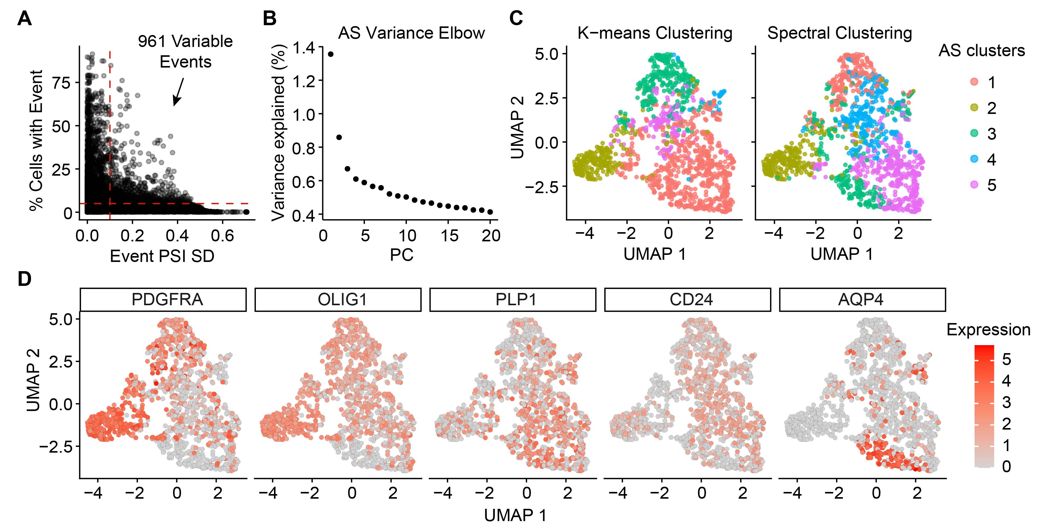
Figure 3. Alternative splicing (AS)-based clustering analysis in pediatric high-grade glioma (pHGG) H3.3K27M tumor cells. (A) Dot plot showing the standard deviation (SD) of percent spliced-in (PSI) values vs. the proportion of cells with detected PSI for each AS event. AS events with PSI SD > 0.1 and detected in more than 5% of cells were considered variable and used for downstream analysis. (B) Elbow plot used to determine the number of principal components for dimensionality reduction based on variable AS events. (C) Uniform manifold approximation and projection (UMAP) plots of tumor cells colored by AS-based clusters identified using K-means (left) and spectral clustering (right). (D) UMAP plots colored by the expression levels of neural lineage–associated marker genes: OLIG1 and PDGFRA for oligodendrocyte precursor cells (OPCs), CD24 for neural progenitor cells (NPCs), PLP1 for oligodendrocytes, and AQP4 for astrocytes, illustrating the association between lineage identity and AS patterns.
6. Perform pairwise differential AS analysis
Pairwise comparisons between AS-based clusters are performed to identify differentially spliced events. Multiple statistical tests—including Kolmogorov–Smirnov, Anderson–Darling, DTS, Wilcoxon, and t-test—are applied, and p-values are adjusted for multiple testing. Analysis is performed separately for each AS event type (SE, MXE, RI, A5SS, A3SS, ALE, AFE), and only events meeting minimum coverage criteria are included. Differential AS events are filtered using an adjusted p-value cutoff of 0.1 and a mean PSI difference cutoff of 10 (Figure 4A).
Note: The min.cells parameter should be optimized for each dataset to ensure sufficient statistical power for differential AS analysis. Additional thresholds, including adjusted p-value and mean PSI difference cutoffs, may also be tuned depending on dataset size and variability, as they can influence the identification of significant events.
method_to_use <- c(“ks”, “ad”, “dts”, “wilcox”, “t.test”)marvel <- CompareValues(MarvelObject = marvel,cell.group.g1 = cell_group_g1,cell.group.g2 = cell_group_g2,min.cells = 20,method = method_to_use,method.adjust = “fdr”,level = “splicing”,event.type = c(“SE”, “MXE”, “RI”, “A5SS”, “A3SS”, “ALE”, “AFE”),show.progress = TRUE)7. Visualize PSI distributions
The exon structures of specific AS events identified from the differential AS analysis and their PSI distributions across glioma AS clusters are visualized to facilitate interpretation of AS patterns (Figure 4B). Detailed scripts to generate these plots are available in Code S3.
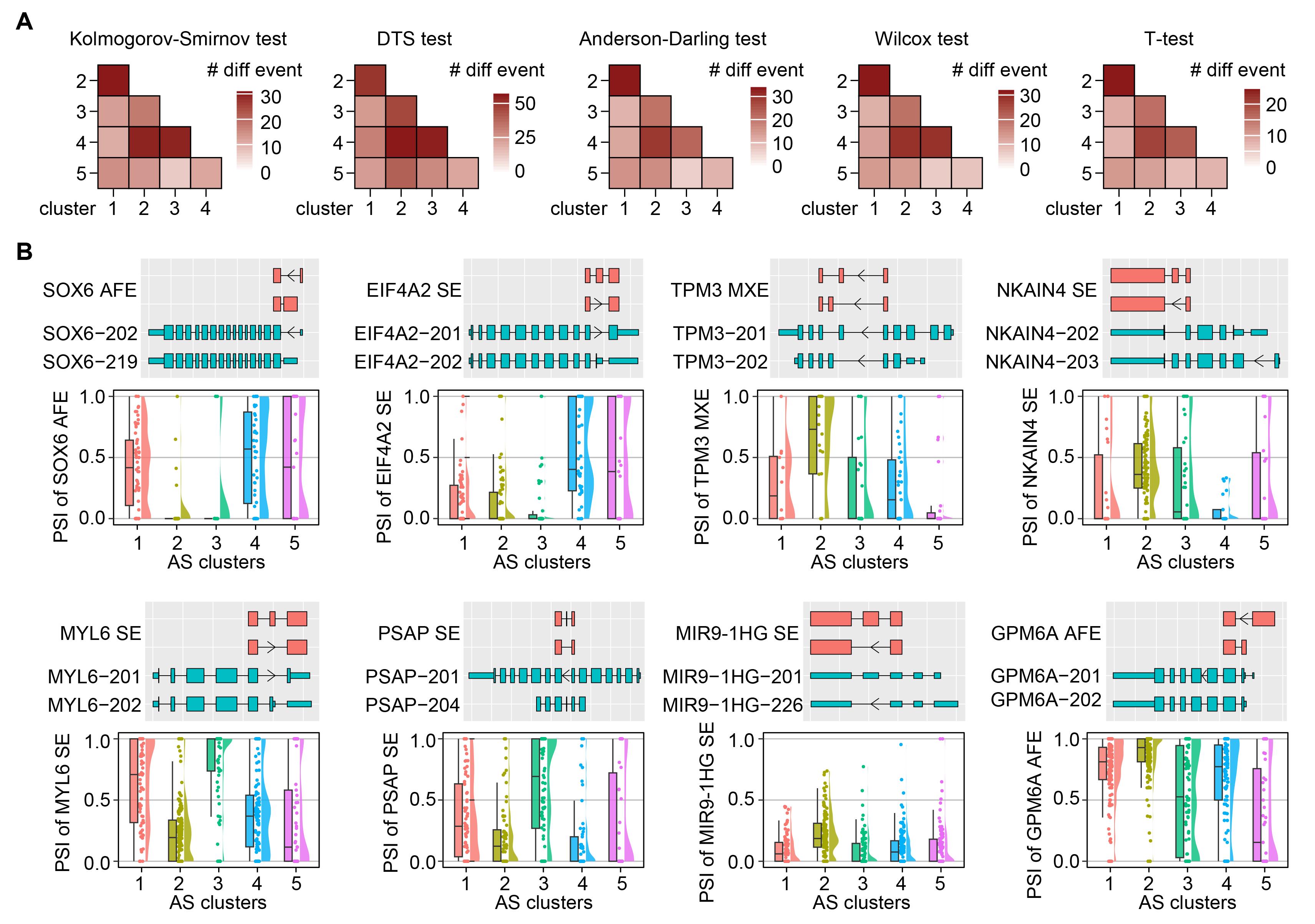
Figure 4. Differential alternative splicing (AS) analysis across AS-based clusters of pediatric high-grade glioma (pHGG) H3.3K27M tumor cells. (A) Heatmaps showing the number of differential AS events identified in pairwise comparisons between AS-based clusters. (B) Schematic diagrams of exon structures and raincloud plots displaying the PSI distributions across AS clusters for selected AS events identified from the differential AS analysis.
Result interpretation
The goal of this example analysis is to identify AS-based clusters in pHGG H3.3K27M tumor cells using scRNA-seq data derived from clinical tumor specimens. To achieve this, gene-level expression data were first used to separate tumor cells from non-tumor cells prior to AS analysis. Gene expression–based clustering revealed transcriptionally distinct populations within the dataset (Figure 2A). Integration of lineage-specific markers with H3F3A mutation status enabled clear delineation of tumor and non-tumor populations, with tumor clusters defined by H3F3A K27M mutation and SOX2 expression (Figure 2B, C). This combined approach ensured accurate identification of tumor cells for downstream AS analysis.
To investigate splicing heterogeneity within tumor cells, AS events with high variability across cells were first identified. Two parameters were used to define variability: the standard deviation of PSI values and the proportion of cells in which the event was detected. Applying the cutoffs described in the procedure, 961 variable AS events were identified (Figure 3A). PCA was then performed on the imputed PSI values of these variable events, and the resulting components were visualized using UMAP, followed by clustering analysis using two methods: K-means [20] and spectral clustering [21] (Figure 3B, C). The expression of neural lineage marker genes—including OLIG1 and PDGFRA for oligodendrocyte precursor cells (OPCs), CD24 for neural progenitor cells (NPCs), PLP1 for oligodendrocytes, and AQP4 for astrocytes—was mapped onto the AS-based UMAP to interpret the relationship between lineage identity and splicing-defined clusters (Figure 3D). Spectral clustering produced clusters that more clearly separated tumor subpopulations and neural lineage identities, making them biologically more interpretable. Differential AS analysis was then performed on the clusters identified by spectral clustering.
Differential splicing analysis across AS-defined clusters revealed that specific cluster comparisons, particularly cluster 1 vs. cluster 2 and cluster 2 vs. cluster 4, consistently exhibited the highest number of differentially spliced events across statistical tests (Figure 4A). These comparisons, therefore, represent the most transcriptionally divergent splicing states within the tumor population. The top differential splicing events identified from these comparisons (Figure 4B) represent high-confidence candidates that may contribute to functional differences between tumor cell subpopulations and serve as targets for downstream mechanistic or therapeutic investigation.
Validation of protocol
This protocol has been used and validated in the following research article:
Song et al. [22] A single-cell atlas of RNA alternative splicing in the glioma-immune ecosystem. Genome Biology (Figure 2A, B, G).
General notes and troubleshooting
General notes
1. This protocol is applicable to datasets generated using full-length scRNA-seq methods, including SMART-Seq2 and other plate-based approaches. Droplet-based approaches (e.g., 10× Genomics) are not supported.
2. Sequencing depth and read coverage are critical determinants of AS detection sensitivity. Datasets with low coverage may result in sparse PSI matrices and reduced power for downstream analyses.
3. Parameter settings, including PSI coverage thresholds, variability cutoffs, number of principal components, and clustering resolution, should be optimized for each dataset. A summary table of key parameters used throughout the workflow, including the rationale for parameter selection, is provided in Table 1.
Table 1. Summary of key parameter settings used in the analysis pipeline
| Step | Function/tool | Parameter/value used | Rationale |
|---|---|---|---|
| B2 | Seurat: subset | nFeature_RNA > 1,000 nFeature_RNA < 15,000 nCount_RNA < 4,000,000 percent.mt < 20 | Dataset-specific filtering criteria were applied to exclude low-quality cells and potential outliers. |
| B6 | Seurat: FindNeighbors | dims = 1:20 | Selected based on elbow plot analysis of principal component variance and prior experience indicating that tumor tissues typically require 15–30 principal components (PCs). |
| B6 | Seurat: FindClusters | resolution = 1.2 | Achieves clear separation of biologically meaningful clusters specific to the dataset. |
| B7 | Seurat: RunUMAP | dims = 1:20 | Matches PCA dimensions selected in B6. |
| C2 | MARVEL: DetectEvents | min.cells = 20, min.expr = 1 | Default MARVEL settings were used. Optimization may be required for individual datasets. |
| C2 | MARVEL: ComputePSI | CoverageThreshold = 10, UnevenCoverageMultiplier = 10 | Default MARVEL settings were used. Optimization may be required for individual datasets. |
| C3 | Set cut-offs for variable AS events | sd_cutoff = 0.1, nonNA_percent_cutoff = 0.05 | Thresholds were selected based on dataset-specific optimization to yield a reasonable number of variable alternative splicing events (500–1,500). |
| C4 | MARVEL: RunPCA | npc.umap = 10 | Parameter optimization is required for each dataset to obtain biologically meaningful clustering. |
| C5 | kmeans, specc | centers = 5 | Parameter optimization is required for each dataset to obtain biologically meaningful clustering. |
| C6 | MARVEL: CompareValues | min.cells = 20 | A minimum of 20 cells per group was required to ensure reliable estimation of AS levels and reduce noise from sparsely represented events. Parameter optimization is required for each dataset. |
4. In this example, tumor and non-tumor cells are distinguished using transcriptome-based clustering together with H3F3A K27M mutation status, since H3F3A is highly expressed and detectable by scRNA-seq. In tumor types with lower mutation expression, alternative strategies such as copy number variation (CNV) analysis can be used to identify tumor cells, for example, with tools like copyKAT [17] or SCEVAN [18].
5. Due to the sparsity and noise inherent to single-cell data, imputation methods (e.g., Bayesian approaches in MARVEL) can improve downstream dimensionality reduction and clustering, but results should be interpreted cautiously. Alternative imputation methods (e.g., kNN, MAGIC, ALRA) can be applied using other packages.
Troubleshooting
Problem 1: Low alignment rate or poor mapping quality.
Possible causes: Low-quality sequencing reads, adapter contamination, or mismatch between reads and reference genome/annotation.
Solutions: Perform quality control using tools such as FastQC and trim adapters or low-quality bases before alignment. Ensure consistency between the genome build (e.g., GRCh38) and GTF annotation. Adjust alignment parameters if needed.
Problem 2: Failure in PSI calculation (e.g., excessive NA values).
Possible causes: Low read support for splice junctions or retained introns; overly stringent filtering parameters.
Solutions: Adjust MARVEL parameters such as CoverageThreshold and UnevenCoverageMultiplier. Filter AS events with low detection rates and retain events with sufficient representation across cells.
Problem 3: Too few variable AS events identified for downstream analysis.
Possible causes: Stringent filtering thresholds or limited biological variability in the dataset.
Solution: Relax thresholds for PSI standard deviation or minimum cell detection (e.g., reduce SD cutoff from 0.1 to 0.05).
Problem 4: PCA or UMAP does not separate cells into meaningful clusters.
Possible causes: Insufficient informative AS features, high noise levels, or suboptimal parameter selection.
Solutions: Reassess variable AS event selection criteria, adjust the number of principal components, and test different UMAP parameters. Confirm that imputation (e.g., Bayesian) is functioning correctly.
Problem 5: Few or no significant differential AS events detected.
Possible causes: Small sample size per cluster, low statistical power, or overly strict filtering thresholds.
Solutions: Ensure sufficient cell numbers per group (e.g., ≥20 cells). Relax adjusted p-value or PSI difference cutoffs if appropriate. Compare results across multiple statistical tests to identify robust events.
Discussion
Multiple computational tools have been developed to identify and analyze AS events from RNA-seq data. While early methods such as MISO [23], rMATS [24], and MAJIQ [25] were primarily designed for bulk RNA-seq analysis, they are not fully optimized for single-cell datasets due to technical limitations including low read coverage, high dropout rates, and increased noise. To address these challenges, several methods have been developed for single-cell splicing analysis, including Expedition [26], BRIE/BRIE2 [27], SCASL [28], SCSES [29], and MARVEL [8]. Each of these tools has its own advantages and limitations. In this context, MARVEL enables quantification of multiple classes of AS events, including SE, MXE, RI, A5SS, and A3SS, as well as two other isoform-level regulatory events, such as AFE and ALE, which are not always supported by other tools. In addition, MARVEL employs a Bayesian-based imputation strategy [19] to address missing PSI values arising from dropout events in single-cell data, which can improve the robustness of downstream component analysis. A key limitation of the MARVEL workflow is that splicing events are defined based on a reference gene annotation. As a result, the analysis is restricted to annotated splicing events and does not capture de novo or novel splicing events. In future studies, systematic benchmarking and comparison of different single-cell splicing analysis pipelines across diverse datasets and biological contexts would be valuable for evaluating their relative performance and guiding optimal method selection.
Supplementary information
The following supporting information can be downloaded here:
1. Code S1. Code for Procedure A: Single-cell RNA-seq data preprocessing
2. Code S2. Code for Procedure B: Gene expression-based clustering and cell type assignment
3. Code S3. Code for Procedure C: AS-based clustering and differential AS analysis
Acknowledgments
Conceptualization, X.S. and S.Y.C.; Investigation, X.S. and M.N.W.; Writing—Original Draft, M.N.W.; Writing—Review & Editing, X.S. and S.Y.C.; Funding acquisition, X.S. and S.Y.C.; Supervision, X.S. and S.Y.C. This work was supported by United States Army Medical Research Acquisition Activity W81XWH-22-1-0374 and HT9425-24-1-0573 (X.S.); NIH NS133160, NS115403, NS125318 (S.Y.C.); Research Funding from Northwestern Medicine Malnati Brain Tumor Institute of the Lurie Cancer Center (X.S.); and Lurie Cancer Center Translational Bridge Training Program (M.N.W.). This protocol was first described and validated in Xiao Song et al. [22]. We thank Northwestern IT Research Computing Services for providing the Quest High-Performance Computing Cluster platform. The following figures were created using BioRender: Graphical overview, https://BioRender.com/2dklrpo; Figure 1, https://BioRender.com/5fel6qe.
Competing interests
The authors declare no competing interests.
References
- Kornblihtt, A. R., Schor, I. E., Alló, M., Dujardin, G., Petrillo, E. and Muñoz, M. J. (2013). Alternative splicing: a pivotal step between eukaryotic transcription and translation. Nat Rev Mol Cell Biol. 14(3): 153–165. https://doi.org/10.1038/nrm3525
- Baralle, F. E. and Giudice, J. (2017). Alternative splicing as a regulator of development and tissue identity. Nat Rev Mol Cell Biol. 18(7): 437–451. https://doi.org/10.1038/nrm.2017.27
- Anczukow, O., Allain, F. T., Angarola, B. L., Black, D. L., Brooks, A. N., Cheng, C., Conesa, A., Crosse, E. I., Eyras, E., Guccione, E., et al. (2024). Steering research on mRNA splicing in cancer towards clinical translation. Nat Rev Cancer. 24(12): 887–905. https://doi.org/10.1038/s41568-024-00750-2
- Zheng, G. X. Y., Terry, J. M., Belgrader, P., Ryvkin, P., Bent, Z. W., Wilson, R., Ziraldo, S. B., Wheeler, T. D., McDermott, G. P., Zhu, J., et al. (2017). Massively parallel digital transcriptional profiling of single cells. Nat Commun. 8(1): e1038/ncomms14049. https://doi.org/10.1038/ncomms14049
- Macosko, E. Z., Basu, A., Satija, R., Nemesh, J., Shekhar, K., Goldman, M., Tirosh, I., Bialas, A. R., Kamitaki, N., Martersteck, E. M., et al. (2015). Highly Parallel Genome-wide Expression Profiling of Individual Cells Using Nanoliter Droplets. Cell. 161(5): 1202–1214. https://doi.org/10.1016/j.cell.2015.05.002
- Picelli, S., Faridani, O. R., Björklund, Ã. K., Winberg, G., Sagasser, S. and Sandberg, R. (2014). Full-length RNA-seq from single cells using Smart-seq2. Nat Protoc. 9(1): 171–181. https://doi.org/10.1038/nprot.2014.006
- Arzalluz-Luque, Ã. and Conesa, A. (2018). Single-cell RNAseq for the study of isoforms—how is that possible?. Genome Biol. 19(1): e1186/s13059–018–1496–z. https://doi.org/10.1186/s13059-018-1496-z
- Wen, W. X., Mead, A. J. and Thongjuea, S. (2023). MARVEL: an integrated alternative splicing analysis platform for single-cell RNA sequencing data. Nucleic Acids Res. 51(5): e29–e29. https://doi.org/10.1093/nar/gkac1260
- Filbin, M. G., Tirosh, I., Hovestadt, V., Shaw, M. L., Escalante, L. E., Mathewson, N. D., Neftel, C., Frank, N., Pelton, K., Hebert, C. M., et al. (2018). Developmental and oncogenic programs in H3K27M gliomas dissected by single-cell RNA-seq. Science. 360(6386): 331–335. https://doi.org/10.1126/science.aao4750
- Dobin, A., Davis, C. A., Schlesinger, F., Drenkow, J., Zaleski, C., Jha, S., Batut, P., Chaisson, M. and Gingeras, T. R. (2012). STAR: ultrafast universal RNA-seq aligner. Bioinformatics. 29(1): 15–21. https://doi.org/10.1093/bioinformatics/bts635
- Putri, G. H., Anders, S., Pyl, P. T., Pimanda, J. E. and Zanini, F. (2022). Analysing high-throughput sequencing data in Python with HTSeq 2.0. Bioinformatics. 38(10): 2943–2945. https://doi.org/10.1093/bioinformatics/btac166
- Quinlan, A. R. and Hall, I. M. (2010). BEDTools: a flexible suite of utilities for comparing genomic features. Bioinformatics. 26(6): 841–842. https://doi.org/10.1093/bioinformatics/btq033
- Li, H., Handsaker, B., Wysoker, A., Fennell, T., Ruan, J., Homer, N., Marth, G., Abecasis, G., Durbin, R., et al. (2009). The Sequence Alignment/Map format and SAMtools. Bioinformatics. 25(16): 2078–2079. https://doi.org/10.1093/bioinformatics/btp352
- Li, B. and Dewey, C. N. (2011). RSEM: accurate transcript quantification from RNA-Seq data with or without a reference genome. BMC Bioinf. 12(1): 323. https://doi.org/10.1186/1471-2105-12-323
- Zafar, H., Wang, Y., Nakhleh, L., Navin, N. and Chen, K. (2016). Monovar: single-nucleotide variant detection in single cells. Nat Methods. 13(6): 505–507. https://doi.org/10.1038/nmeth.3835
- Hao, Y., Stuart, T., Kowalski, M. H., Choudhary, S., Hoffman, P., Hartman, A., Srivastava, A., Molla, G., Madad, S., Fernandez-Granda, C., et al. (2023). Dictionary learning for integrative, multimodal and scalable single-cell analysis. Nat Biotechnol. 42(2): 293–304. https://doi.org/10.1038/s41587-023-01767-y
- Gao, R., Bai, S., Henderson, Y. C., Lin, Y., Schalck, A., Yan, Y., Kumar, T., Hu, M., Sei, E., Davis, A., et al. (2021). Delineating copy number and clonal substructure in human tumors from single-cell transcriptomes. Nat Biotechnol. 39(5): 599–608. https://doi.org/10.1038/s41587-020-00795-2
- De Falco, A., Caruso, F., Su, X. D., Iavarone, A. and Ceccarelli, M. (2023). A variational algorithm to detect the clonal copy number substructure of tumors from scRNA-seq data. Nat Commun. 14(1): 1074. https://doi.org/10.1038/s41467-023-36790-9
- Benegas, G., Fischer, J. and Song, Y. S. (2022). Robust and annotation-free analysis of alternative splicing across diverse cell types in mice. eLife. 11: e73520. https://doi.org/10.7554/elife.73520
- Ikotun, A. M., Ezugwu, A. E., Abualigah, L., Abuhaija, B. and Heming, J. (2023). K-means clustering algorithms: A comprehensive review, variants analysis, and advances in the era of big data. Inf Sci. 622: 178–210. https://doi.org/10.1016/j.ins.2022.11.139
- Ng, A. Y., Jordan, M. I. and Weiss, Y. (2002). On spectral clustering: Analysis and an algorithm. Adv Neur In 14: 849–856.
- Song, X., Tiek, D., Lu, M., Yu, X., Wu, R., Walker, M., He, Q., Sisbarro, D., Hu, B., Cheng, S. Y., et al. (2025). A single-cell atlas of RNA alternative splicing in the glioma-immune ecosystem. Genome Biol. 26(1): 426. https://doi.org/10.1186/s13059-025-03889-9
- Katz, Y., Wang, E. T., Airoldi, E. M. and Burge, C. B. (2010). Analysis and design of RNA sequencing experiments for identifying isoform regulation. Nat Methods. 7(12): 1009–1015. https://doi.org/10.1038/nmeth.1528
- Shen, S., Park, J. W., Lu, Z. x., Lin, L., Henry, M. D., Wu, Y. N., Zhou, Q. and Xing, Y. (2014). rMATS: Robust and flexible detection of differential alternative splicing from replicate RNA-Seq data. Proc Natl Acad Sci USA. 111(51): e1419161111. https://doi.org/10.1073/pnas.1419161111
- Vaquero-Garcia, J., Aicher, J. K., Jewell, S., Gazzara, M. R., Radens, C. M., Jha, A., Norton, S. S., Lahens, N. F., Grant, G. R., Barash, Y., et al. (2023). RNA splicing analysis using heterogeneous and large RNA-seq datasets. Nat Commun. 14(1): 1230. https://doi.org/10.1038/s41467-023-36585-y
- Song, Y., Botvinnik, O. B., Lovci, M. T., Kakaradov, B., Liu, P., Xu, J. L. and Yeo, G. W. (2017). Single-Cell Alternative Splicing Analysis with Expedition Reveals Splicing Dynamics during Neuron Differentiation. Mol Cell. 67(1): 148–161.e5. https://doi.org/10.1016/j.molcel.2017.06.003
- Huang, Y. and Sanguinetti, G. (2021). BRIE2: computational identification of splicing phenotypes from single-cell transcriptomic experiments. Genome Biol. 22(1): e1186/s13059–021–02461–5. https://doi.org/10.1186/s13059-021-02461-5
- Xiang, X., He, Y., Zhang, Z. and Yang, X. (2024). Interrogations of single-cell RNA splicing landscapes with SCASL define new cell identities with physiological relevance. Nat Commun. 15(1): e1038/s41467–024–46480–9. https://doi.org/10.1038/s41467-024-46480-9
- Wen, X., Lv, X., Guo, D., Han, N., Zhou, L., Wang, P. and Liu, Z. (2025). Deciphering splicing heterogeneity at single-cell resolution by SCSES. Nat Commun. 16(1): e1038/s41467–025–64517–5. https://doi.org/10.1038/s41467-025-64517-5
Article Information
Publication history
Received: Mar 30, 2026
Accepted: May 25, 2026
Available online: Jun 3, 2026
Published: Jun 20, 2026
Copyright
© 2026 The Author(s); This is an open access article under the CC BY-NC license (https://creativecommons.org/licenses/by-nc/4.0/).
How to cite
Walker, M. N., Hu, B., Cheng, S. and Song, X. (2026). Stepwise Protocol for Alternative Splicing Analysis in Single-Cell SMART-Seq2 RNA-Seq Data. Bio-protocol 16(12): e5735. DOI: 10.21769/BioProtoc.5735.

 Download Citation in RIS Format
Category
Bioinformatics and Computational Biology
Molecular Biology > RNA > RNA splicing
Systems Biology > Transcriptomics > RNA-seq
Do you have any questions about this protocol?
Post your question to gather feedback from the community. We will also invite the authors of this article to respond.
 Post a Question


