


- Protocols

- Articles and Issues
- For Authors
- About
- Become a Reviewer


Protocol for In Vivo Two-Photon FCS to Measure Nanocarrier Number and Flow Velocity in Mouse Cerebral Microvasculature


Published: Vol 16, Iss 13, Jul 5, 2026 DOI: 10.21769/BioProtoc.5717 Views: 263
Reviewed by: Olga KopachJordi Boix-i-CollRupam Ghosh
 PDF
PDF  Ask a question
Original research article
The authors used this protocol in:
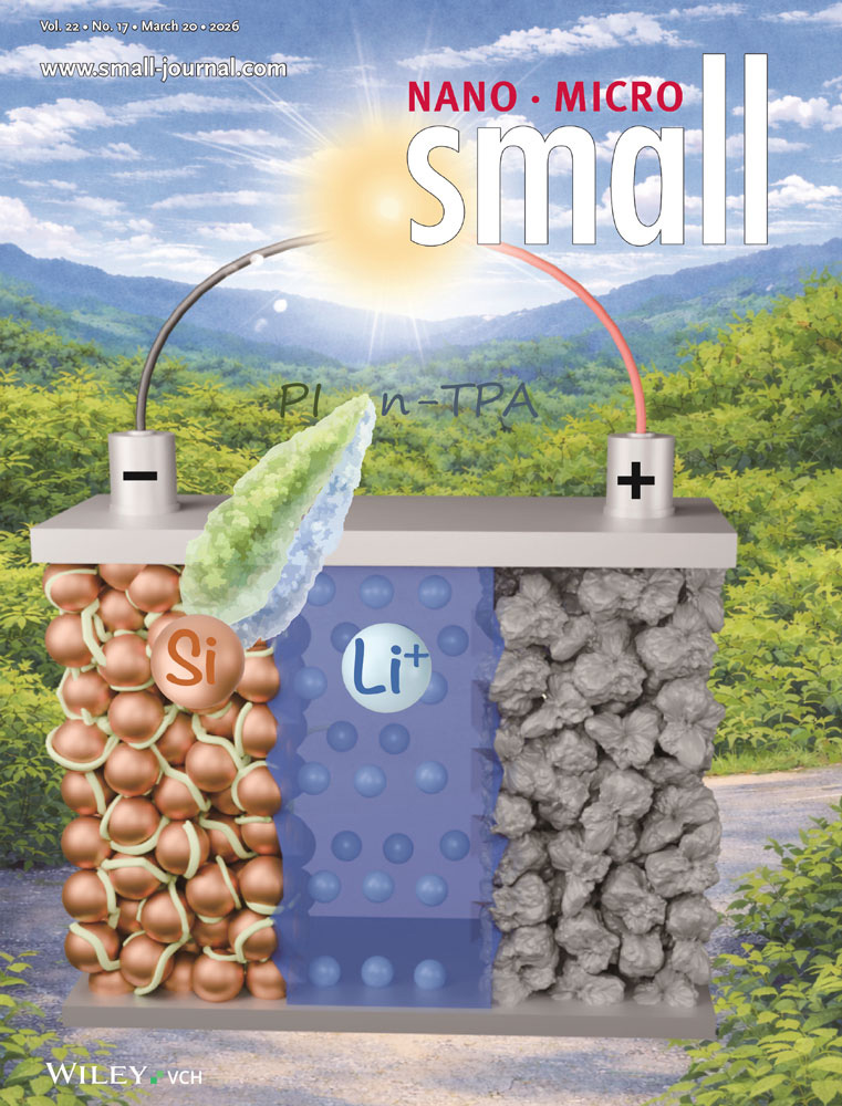
Mar 2026
Advertisement


Protocol Collections
Comprehensive collections of detailed, peer-reviewed protocols focusing on specific topics




Abstract
Real-time measurement of blood flow and nanocarrier transport in the cerebral microvasculature is crucial for understanding neurovascular physiology and nanocarrier-based drug delivery. Existing techniques lack the ability to measure blood flow rates in individual vessels with high spatial and temporal resolution in real time. Two-photon fluorescence correlation spectroscopy (2P-FCS) provides a powerful approach for monitoring tracer molecules within a small confocal observation volume. This enables the simultaneous determination of particle number and flow dynamics in vivo. Here, we present a detailed protocol for in vivo 2P-FCS measurements in the mouse cerebral microvasculature. The protocol includes preparation of the cranial window, delivery of fluorescent dextran tracers for vascular visualization, and FCS measurements. It also includes two-photon imaging of the cerebrovascular network and acquisition and analysis of fluorescence correlation data. The protocol describes calibration of the confocal volume diameter and optimization of two-photon excitation parameters. This workflow enables real-time measurement of tracer concentration and flow velocity in individual cerebral microvessels with high spatial and temporal resolution. The method can be adapted to study blood flow dynamics, nanoparticle transport, and microvascular physiology in a variety of in vivo imaging systems equipped with multiphoton microscopy and FCS capabilities.
Key features
• Protocol for performing in vivo 2P-FCS for real-time measurements of nanocarrier flow and concentration in the mouse cerebrovasculature through an acute cranial window.
• Provides guidance on calibrating the confocal volume diameter and optimizing near-infrared (NIR) laser power and excitation wavelengths of fluorophores.
• Includes procedures for two-photon imaging of cerebral blood vessels.
• Applicable to studies of cerebral blood flow, nanoparticle transport, and microvascular dynamics using multiphoton microscopy systems equipped with FCS modules.
Keywords: Fluorescence correlation spectroscopy (FCS) Multiphoton microscopy
Cerebral microvasculature
In vivo Imaging
Nanocarrier transport
Cerebral blood flow
Multiphoton microscopy
Cerebral microvasculature
In vivo Imaging
Nanocarrier transport
Cerebral blood flow
Graphical overview
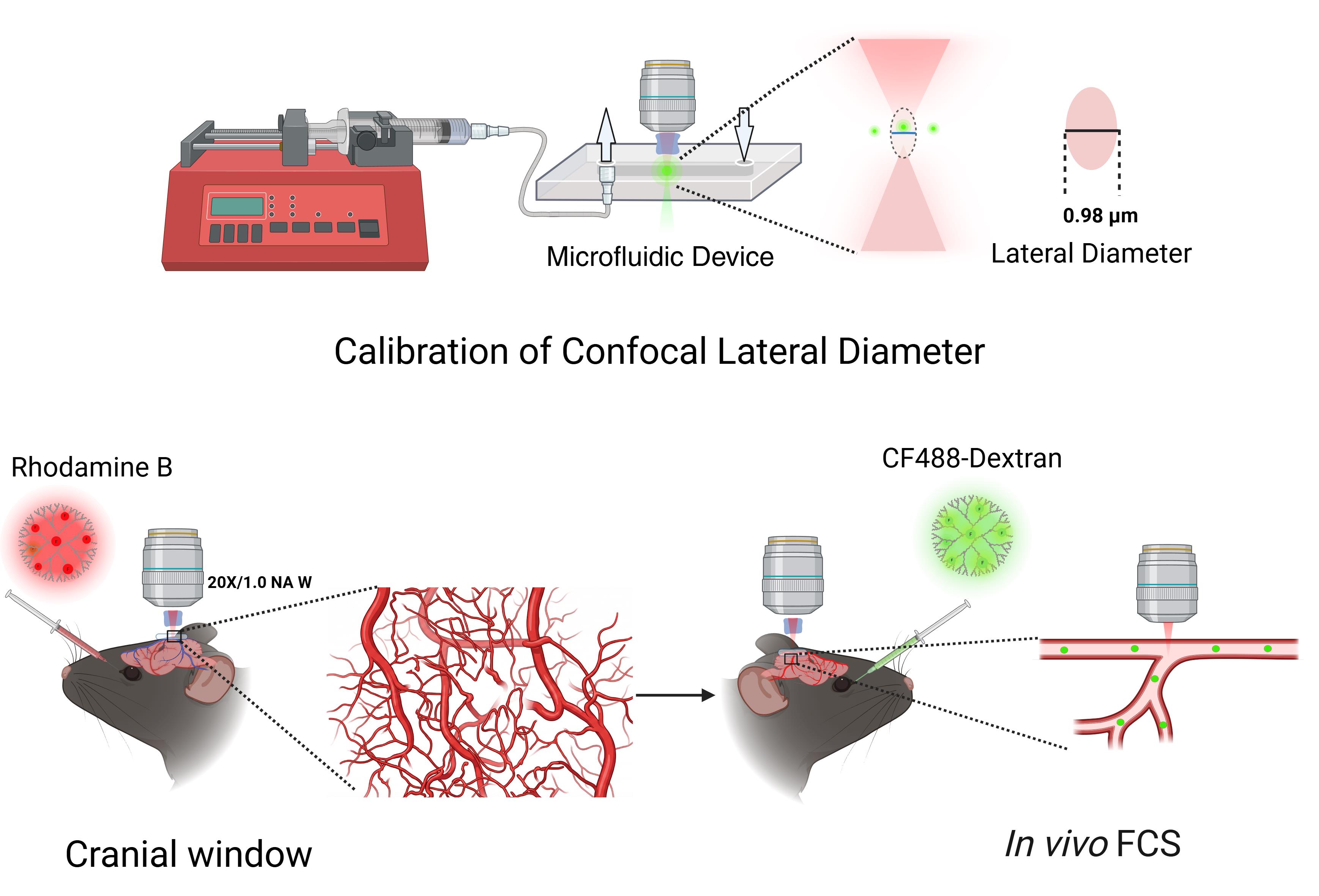
Workflow for in vivo two-photon fluorescence correlation spectroscopy (2P-FCS) measurements in mouse cerebrovasculature
Background
Cerebral blood vessels, such as veins, arteries, and capillaries, form the cerebrovascular network and are responsible for a variety of functions, including ion exchange regulation, molecular and oxygen transport, and waste removal [1]. Cerebral blood flow (CBF), particularly in capillaries, provides vital information about the central nervous system’s functionality. For instance, abnormalities in CBF patterns can indicate conditions such as ischemic stroke when blood flow slows down, brain tumors when flow patterns alter, or neurodegenerative diseases like Alzheimer's when CBF gradually declines [2,3]. Thus, CBF assessment can reveal how the brain’s autoregulation system maintains stable blood flow despite systemic changes in blood pressure. Various techniques, such as computed tomography (CT) [4], magnetic resonance imaging (MRI) [5], and fluorescence imaging [6,7] have been developed for measuring CBF. However, real-time measurement of blood flow rates in individual vessels using these existing technologies is challenging, especially in capillaries (<10 μm), due to their limited spatial resolution [8]. While CT and MRI provide whole-brain perfusion measurements, they lack the spatial resolution required to resolve capillary-scale flow dynamics [9,10]. Optical techniques such as laser speckle imaging and Doppler optical coherence tomography improve temporal resolution but do not achieve single-capillary sensitivity or single-particle detection [8,11]. Multiphoton laser-scanning microscopy (MPLSM) techniques can measure flow rates when a two-photon fluorescence dye provides contrast against red blood cells (RBCs). However, these approaches require line-scanning over vessel segments and are limited by scan speed, which prevents pixel-level flow readout and reduces temporal precision [12,13]. Furthermore, intensity-based imaging methods cannot directly quantify nanocarrier concentration or number in real time.
Fluorescence correlation spectroscopy (FCS) is a single-molecule-sensitive technique that measures and correlates the fluctuations of fluorescent molecules diffusing through a defined detection volume, often called the confocal volume. The correlation from fluctuations in fluorescent molecules provides information such as the molecules' diffusion time, surface binding, and the number of molecules within the confocal volume. The strength of FCS lies in its ability to distinguish the uncorrelated background from the correlated signal [14,15]. FCS has previously been widely applied for in vitro applications, including in microfluidic devices, but has now been expanded to study flow and diffusion dynamics in thick biological tissues using multiphoton excitation. By leveraging deeper penetration and reducing out-of-focus excitation artifacts of two-photon (2P) microscopy, in vivo FCS was used to measure pixel-by-pixel blood flow velocity in live mice. For example, Xu et al. employed FCS to measure CBF in live mice using optimized two-photon fluorophores with high spatial and temporal resolution at a depth of 300 μm within brain tissue [16]. Further developments in cerebral blood flow measurements were reported by Xiaojin et al., who used near-infrared-emitting DNA-stabilized silver nanoclusters (DNA-AgNCs) [17]. The liposomes-encapsulated near-NIR DNA-AgNCs showed a better spectral crosstalk with the blood vessel-lighting dye FITC. A recently published article by the same author shows that flow rate measurements were further improved by chronically labeling the cerebrovasculature with adeno-associated viral vectors (AAV) encoding albumin-mNeonGreen (Alb-mNG) expression [18]. A nanocarrier composed of loaded DNA-AgNCs, encapsulated in liposomes and loaded into cationic mesoporous silica nanoparticles, was used as an FCS probe for measuring cerebral blood flow. These studies established the feasibility of quantitative, real-time measurements of nanocarrier dynamics in the cerebrovasculature. Despite these published articles, guidance on the reproducibility of in vivo two-photon FCS remains challenging due to the complexity of the experimental procedures. Many experimental parameters, such as excitation and emission spectra for 2P dyes, confocal volume calibration, cranial window preparation, and correlation-based velocity extraction, among others, need to be optimized and are briefly described in the published articles. However, troubleshooting techniques to minimize motion artifacts are not discussed in detail in such articles. Hence, a step-by-step experimental procedure is needed to ensure the reproducibility of in vivo FCS measurements for the quantification of nanocarrier number in the cerebrovasculature.
The protocol described here provides detailed, reproducible experimental procedures for performing in vivo two-photon fluorescence correlation spectroscopy (2P-FCS) to measure the number of nanocarriers and their flow velocity in the mouse cerebral microvasculature in real time. This includes optimization of two-photon excitation, microfluidic calibration, cranial window preparation, and flow-diffusion autocorrelation modeling to determine absolute particle concentration and transport dynamics in real time. The benefit of this protocol is that it works well for a wide range of fluorescent nanocarriers, including dextran conjugates, liposomes, and polymeric nanoparticles. This technique can be used with various two-photon imaging systems that have photon-counting detectors. It is especially beneficial for researchers studying nanomedicine pharmacokinetics, cerebral blood flow, vascular transport dynamics, and in vivo nanoparticle clearance. Compared to earlier published in vivo FCS protocols, this one offers (i) a microfluidic calibration process to convert correlation decay times to absolute flow velocities, (ii) practical strategies to reduce motion artifacts in live animals, and (iii) a detailed data analysis framework for extracting both particle number and velocity from the same autocorrelation curve. Beyond cerebral blood flow measurement, this protocol can be adapted to investigate nanocarrier pharmacokinetics, blood–brain barrier transport, vascular permeability, tumor microvascular dynamics, and nanoparticle clearance in real time. By providing a standardized methodological framework, this protocol facilitates broader adoption of in vivo two-photon FCS for quantitative vascular and nanomedicine research.
Materials and reagents
Biological materials
1. Mice (C57BL/6), 5-6 months old, both male and female (The Jackson Laboratory, catalog number: 000664; stored in the institutional animal facility under standard housing conditions)
Reagents
1. FITC-dextran, 70 kDa (Millipore Sigma, CAS number: 60842-46-8); store at -20 °C and protect from light
2. CF488A-dextran, 250 kDa (Biotium, catalog number: 80117); store at -20 °C and protect from light
3. Rhodamine B-dextran, 70 kDa (Thermo Fisher Scientific, catalog number: D1841); store at -20 °C and protect from light
4. Phosphate-buffered saline (PBS), 20×, pH 7.4 (Thermo Fisher Scientific, catalog number: 28348); store at room temperature
5. Isoflurane (size: 250 mL) (Piramal Healthcare), store at 15–30 °C
6. Meloxicam 5 mg/mL (Entirely Pets Pharmacy, catalog number: MWI119887); store at 20 °C
7. Dexamethasone sodium phosphate (Sigma-Aldrich, catalog number: D2915); store at 4 °C
8. Bupivacaine hydrochloride, 0.25% (Meitheal, NDC: 71288-723-52)
9. Sterile 0.9% saline solution (Baxter, catalog number: 2B1324); store at room temperature
10. Deionized water (18.2 MΩ·cm) (Millipore system)
11. Gelfoam absorbable gelatin sponge (Pfizer, catalog number: 00009031501)
12. Chlorhexidine solution 0.2% (Heartland Vet Supply & Pharmacy, catalog number: 71142)
13. 70% ethanol wipes (Uline, catalog number: S-18560)
14. GenTeal tears lubricant eye gel (Alcon, NDC: 0065-8064-01)
Solutions
1. 1× PBS, pH 7.4 (see Recipes)
2. Rhodamine B-dextran (70 kDa) working injection solution (see Recipes)
3. CF488-dextran (250 kDa) working injection solution (see Recipes)
Recipes
1. 1× PBS, pH 7.4
| Reagent | Final concentration | Quantity or volume |
|---|---|---|
| 10× PBS | 1/10 | 10 mL |
| MilliQ H2O | n/a | 90 mL |
| Total | 1× | 100 mL |
2. Rhodamine B-dextran (70 kDa) working injection solution
| Reagent | Final concentration | Quantity or volume |
|---|---|---|
| Rhodamine B-dextran | 10 mg/mL | 100 μL |
| 1× PBS | n/a | 100 μL |
| Total | 5 mg/mL | 200 μL |
3. CF488-dextran (250 kDa) working injection solution
| Reagent | Final concentration | Quantity or volume |
|---|---|---|
| CF488-dextran | 10 mg/mL | 1 μL |
| 1× PBS | n/a | 99 μL |
| Total | 0.1 mg/mL | 100 μL |
Laboratory supplies
1. Round glass coverslips, 5 mm diameter (Fisher Scientific, catalog number: 50-949-439)
2. Scalpel blades, No. 10 (Integra Miltex, catalog number: 4-110)
3. Surgical scissors (Fine Science Tools, catalog number: 14001-12)
4. Fine forceps (Fine Science Tools, catalog number: 11251-10)
5. 1 mL syringes (BD, catalog number: 309659)
6. 27 G insulin syringes (BD, catalog number: 328468)
7. 0.22 μm syringe filters (Millipore, catalog number: SLGP033RS)
8. Dental cement (Parkell C&B Metabond, catalog number: S380)
9. Cyanoacrylate adhesive (Loctite 401)
10. 96-well glass bottom plates (Cellvis, catalog number: P96-1.5H-N)
11. Elbow Luer connector male (ibidi, catalog number:10802)
12. Luer connector female (ibidi, catalog number:10825)
13. Biocompatible silicone tubing (ibidi, catalog number: 10840)
14. MAT professional-grade wide electrical tape white (Amazon, 1.5 inch× 66 ft.)
15. 25 × 25 mm No. 1.5 coverslip (VWR, catalog number: 48366-249)
16. Greiner Petri dish (Sigma-Aldrich, catalog number: 664161)
17. O-Ring Kit (Great Western Seal and Gasket, model: O-KIT-568-N70-436-36)
18. Cotton tip applicators (Medline, catalog number: MIIMDS202105)
Equipment
1. Two-photon laser scanning microscope (Zeiss LSM 880 NLO, Carl Zeiss Microscopy, model: LSM 880)
2. Tunable femtosecond pulsed laser (Spectra Physics X3 or equivalent, 140 fs, 80 MHz repetition rate)
3. Water-immersion objective lens (Zeiss 20×/1.0 NA W Plan-Apochromat)
4. Photon-counting detector (Becker & Hickl SPC module or equivalent TCSPC system)
5. Hardware correlator (ALV-7004 or equivalent)
6. Isoflurane vaporizer system (VetEquip, model: 911103)
7. Heating pad with temperature controller (Harvard Apparatus, catalog number: 50-7059)
8. Dental drill with micro-burr (Foredom, model: K.1070)
9. Flex Station 3 microplate reader (Molecular device, model: FLEX3)
10. Digital handheld optical power and energy meter consoles (THOR LABS, model: PM100D2)
11. Sticky-Slide I0.2 Luer (ibidi, catalog number: 80176)
12. Single-channel syringe pump (United States Plastic Corp., catalog number: 98242)
13. Optical power sensor (Thorlabs, model: PM100D or equivalent)
14. Stereotaxic frame/head holder (Kent Scientific or equivalent)
15. Laser safety curtain with smart table (Newport, model: OTS-LSC-512)
16. Mouse Surgical Kit (a complete 7-piece surgical set for mice) (Kent Scientific, model: INSMOUSEKIT)
17. 525/50 nm bandpass filter (Semrock, custom order)
18. 590/100 nm bandpass filter (Semrock, custom order)
19. Dichroic mirror (Carl Zeiss, model: BS MP 760)
Software and datasets
1. Zen Black 2.3 (Carl Zeiss Microscopy, Germany), released in 2018; requires a commercial license provided with the Zeiss LSM 880 microscope system.
2. Microsoft Excel 365 (Microsoft, USA), released in 2023; a commercial license is required.
Procedure
A. Dye pair selection and single-photon emission spectra measurement
Dye pairs are required to have sufficient two-photon absorption cross-sections to make them visible within the vasculature and must be spectrally separated with minimal crosstalk to enable simultaneous vascular imaging and in vivo FCS measurements. In this protocol, we propose two spectrally separated dyes, CF488 (emission at 517 nm) and Rhodamine B (emission at 592 nm). Rhodamine B-dextran is used to illuminate the blood vessels, and CF488-dextran nanoparticle is used for the FCS probe. The measurement of the emission profiles of both dyes will allow us to define the optical window for two-photon excitation and in vivo FCS experiments (Figure 1).
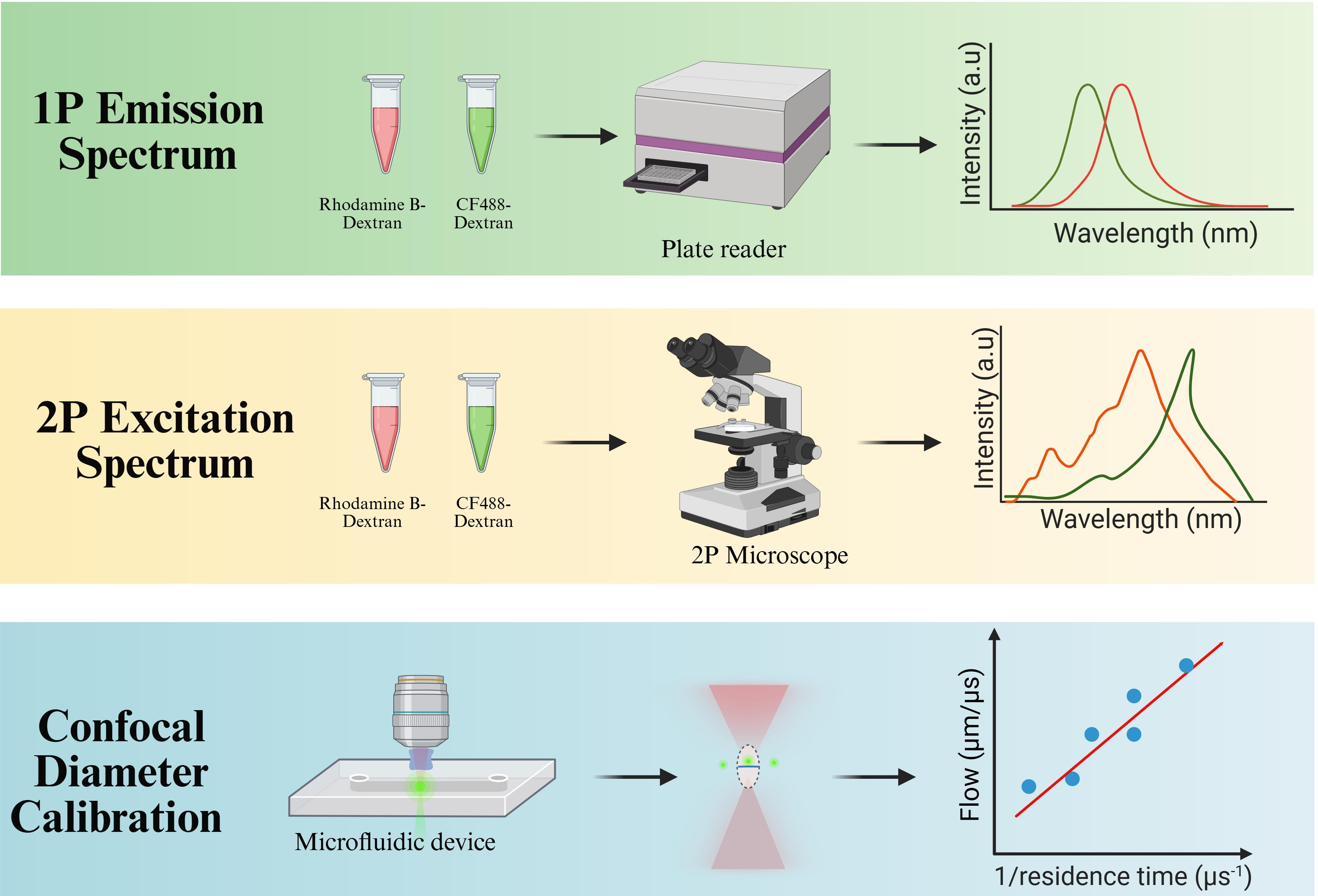
Figure 1. Workflow for dye pair selection, two-photon (2P) excitation characterization, and confocal volume diameter calibration
1. Prepare a very low concentration of 0.005 mg/mL solutions of CF488-dextran (250 kDa) and Rhodamine B-dextran (70 kDa) in 1× PBS buffer.
2. Take 200 μL of diluted solution of CF488 dextran (250 kDa) and Rhodamine B-dextran (70 kD) in a black 96-well glass-bottomed plate.
3. Excite CF488-dextran with 450 nm excitation light and collect the emission from 470 to 600 nm.
4. Similarly, excite Rhodamine B with 500 nm light and collect the emission from 520 to 700 nm.
5. Measure the emission of both dyes in the plate reader fluorescence device. For example, we used the Flex Station 3 Microplate reader.
6. Export the data from the plate reader software to Excel or text format.
7. Plot the emission intensity (relative fluorescence unit) against the wavelength (nm) of both dyes in Excel or any equivalent graphical software. A representative graph is shown in Figure 2.
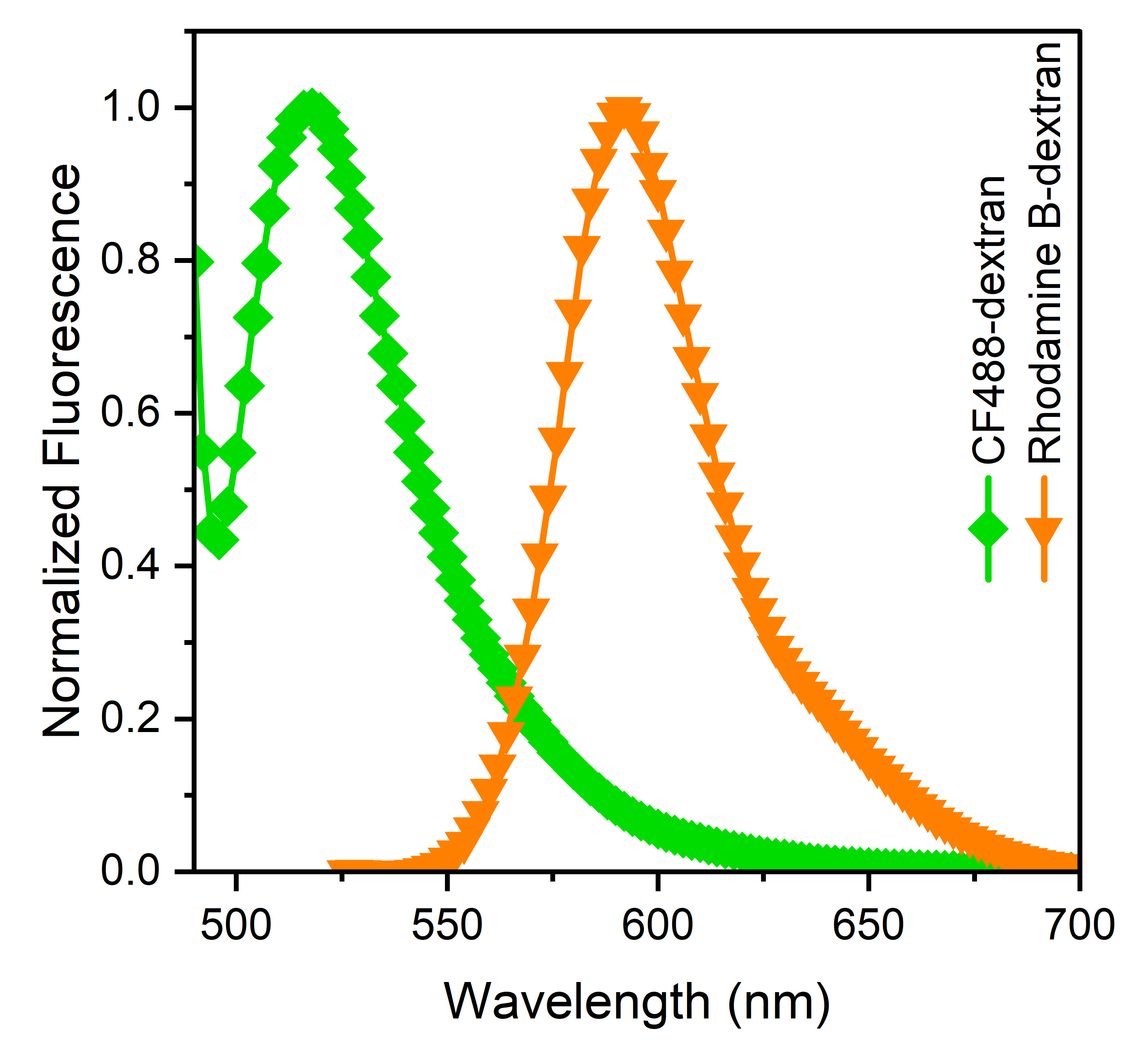
Figure 2. Emission spectra of CF488-dextran and Rhodamine B-dextran
B. 2P excitation spectrum measurement using an upright confocal laser scanning microscope
While 2P spectra and absorption cross-sections of some common dyes have been reported in the literature [19–21], we recommend measuring 2P spectra of the pair of dyes used for in vivo FCS under the given microscope setup.
B1. Measurement of NIR laser power
The output laser power of the excitation wavelengths must be calibrated to maintain constant power at the sample during spectral acquisition. This is because measuring the 2P excitation spectrum of a fluorophore requires scanning the sample in the NIR and collecting fluorescence at a fixed excitation power. Since the output power of tunable femtosecond lasers varies across the NIR range, it is important to precisely measure laser power at different excitation wavelengths.
1. Connect the optical power sensor to the power meter as described in the manual instructions.
2. Place the power sensor on the microscope stage directly beneath the objective lens (10×/0.5 NA) and secure the sensor to the microscope stage using laboratory tape to prevent movement.
3. Turn on the power meter and allow it to stabilize for several minutes.
4. Set the excitation wavelength of the tunable femtosecond laser to 750 nm.
5. Set the same wavelength of 750 nm in the power meter and turn the laser on.
6. Adjust the laser output using the microscope control software (details of the software described in section B3) until the power meter reads 10 mW at the sensor. Record the laser power percentage in a spreadsheet.
7. Change the excitation laser wavelength to 760 nm. Adjust the laser output until the power meter reads 10 mW.
Critical: Ensure the laser beam is completely within the power sensor's active area.
8. Record the corresponding laser power percentage from the software.
9. Repeat this process at 10 nm intervals across the desired wavelength range (e.g., 750–1,200 nm).
10. Compile the recorded power settings for each wavelength into a spreadsheet (e.g., Microsoft Excel). Use this calibration matrix during the acquisition of two-photon excitation spectra to ensure consistent excitation power across all wavelengths.
Note: The target laser power (e.g., 10 mW) can be adjusted depending on fluorophore brightness and photobleaching sensitivity.
B2. Sample channel preparation (O-ring sandwich)
1. Place one #1.5 coverslip on a clean Petri dish surface.
2. Place an O-ring on the coverslip.
3. Pipette ≥300 μL of fluorophore solution into the O-ring well (volume may vary with O-ring size; ensure complete filling).
4. Carefully place the second #1.5 coverslip on top to form a sealed channel.
5. Check for bubbles. If bubbles are present, gently tap the channel or remake it.
B3. Microscope configuration and measurement of 2P spectra
1. Select the emission detection filter appropriate for your dye: collect emission in the green channel through a 525/50 nm bandpass filter for CF488-dextran and collect emission in the red channel through a 590/100 nm bandpass filter.
2. Insert the NIR dichroic mirror (e.g., BS MP 760) into the microscope.
3. Open Zeiss Zen Black software and navigate to the Acquisition tab. Load the NDD800 default setting from the Experiment Manager.
4. Select a 10×/0.5 NA long working distance objective and focus within the solution.
5. Now, select the 750 nm wavelength, set the laser power to achieve 10 mW, and turn on live imaging mode.
6. Lower the objective and adjust its position downward using the focusing knob. Turn the Live mode off when the solution is focused.
7. Now, go to the FCS tab on Zeiss software and select the multiphoton light path. If the light path is not configured in the system, you can set it up as shown in Figure 3. Give it a name, such as “RhodGreen.”
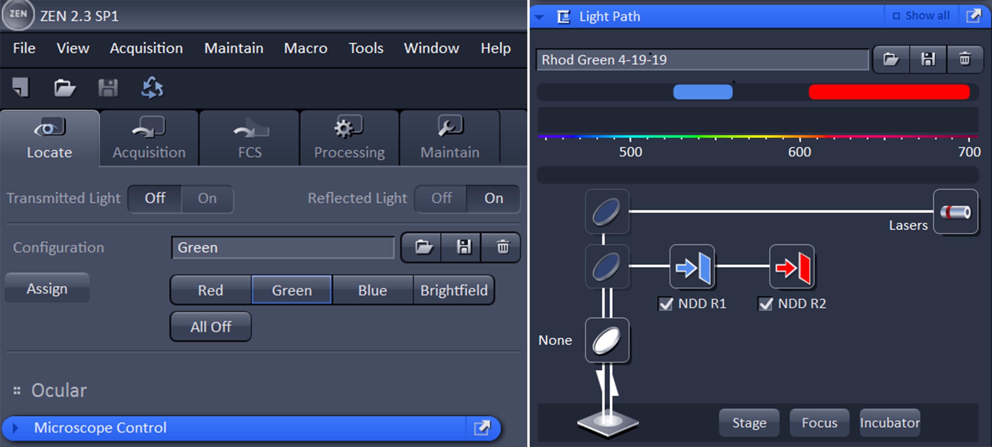
Figure 3. Common tabs and light path configuration for two-photon fluorescence correlation spectroscopy (2P-FCS) using Zen Black Software
8. Set the laser excitation wavelength to the start value (e.g., 775 nm) and set the excitation power to a constant value (10 mW).
9. Click on the count rate on the FCS tab and record the fluorescence intensity (kHz) at that wavelength.
Caution: Ensure the detector is not saturated at any wavelength.
10. Increase the excitation wavelength in 10 nm steps, repeat acquisition, and continue through the full range (e.g., 775–1,100 nm).
11. Save the dataset with metadata (wavelength, power, detector settings, emission filter).
12. Plot the wavelength vs. fluorescent count in a spreadsheet. In our optical setup, the wavelength corresponding to the maximum absorption of CF488 and Rhodamine B was 920 and 850 nm, respectively.
C. Calibration of the confocal lateral diameter using microfluidic channels
The lateral diameter of the confocal volume (d) can be determined from the velocity (v) and the flow residence time (τf) based on the following equation: d = τf × v. Therefore, to calibrate the focal volume, the CF488-dextran particles will flow through a microfluidic channel of known dimensions at different flow rates. The flow velocity (v) will be calculated from known flow rates and channel dimensions. The flow residence time (τf) will be extracted from the fitting of the autocorrelation function. The slope of the linear fitting lines between flow velocity and the reciprocal of residence time will represent the calibrated lateral diameter. The graphical abstract provides a general schematic overview of the calibration.
C1. Preparation of the flow system
1. Load 5 mL of CF488-dextran in a 10 mL syringe. The concentration of the solution should be around 1 × 10¹⁰ particles/mL.
2. Place the pump on the microscope stage and plug it into the power source.
3. Connect the microfluidic flow channel with the inlet and outlet tubing. Then, connect the inlet tubing to the syringe.
4. Place a sample collector beneath the stage and insert the outlet tubing into a collector tube.
5. Mount the syringe on the pump and set the flow rate to 0.05 mL/min.
6. Turn the pump on for 1 min and check the setup before starting the experiment. Ensure there are no air bubbles inside the flow channel.
C2. Microscope setup and focusing
1. Select the 20× objective lens (water immersion objective) from the turret or use an equivalent long working distance objective.
2. Lower the objective carefully using the coarse focus knob. Make sure that the objective lens does not hit the flow channel. Make a reasonable gap between the objective and the flow channel.
3. Open the ZEN black software.
4. Go to the software, click the Locate tab, and select an LED light, e.g., green. You will see a light spot by your eye that illuminates the flow channel.
5. Adjust the stage with the joystick and make sure the focus is on the middle of the flow channel.
6. Now, turn off the LED from the Locate tab.
7. Add two drops of water between the objective and the flow channel. Make sure the water is connected to the objective and flow channel by its viscosity.
8. Now, raise the objective height a little bit with the fine-focusing knob.
9. Go to the software’s Acquisition tab and start Live.
10. Using the fine-focusing knob, move the objective down; you will be able to see some reflection on the computer screen. Keep going slowly; when the screen becomes white, stop here. This is the first reflection plan for water immersion at the glass-flow channel interface.
11. Repeat the same process to get the reflection of the second interface between the sample and the glass of the flow channel. Now, finally, move the objective down to a Z-position of -80 to -90.
Caution: Gradually turn down the objective using only the fine knob; quick adjustments may miss the reflection from the glass interface.
C3. FCS measurement
1. From the Experiment Manager, change to a light path configuration designed for two-photon excitation.
2. Insert the dichroic mirror into the microscope.
3. Cover the microscope with a black curtain and then turn off the room light.
4. Go to the FCS tab and from the Experiment manager, select RhodGreen.
5. Go to the Light Path option. Here, you have two major beam splitters: one for visible light and one for invisible light (if applicable). Check the configuration to ensure the invisible light is directed to the Big3 detector.
6. Select Plate in front of the Visible Light (if applicable). It is a two-photon FCS; hence, we do not need to use visible light.
7. Check MBS 760+ in front of Invisible Light. The MBS reflects the specified laser lines and allows the resulting fluorescence spectrum to pass through.
8. Go to the Acquisition under the FCS tab. Select a 920 nm excitation laser with power corresponding to 10 mW (use your previously made matrix).
9. Set the FCS acquisition time to 10 s with 10 repetitions.
10. Now, start the pump at a flow rate of 0.005 mL/min.
11. Open the Count Rate window by clicking the Count Rate action button in the FCS tab. A good starting point is to set the intensity so that the count rate is between 50 and 200 kHz.
12. When the count is below the limit of both channels, you can click the icon of Start Experiment.
13. After running the experiment, save the file.
14. Now, repeat steps C3.11–13 for 0.1, 0.2, 0.3, 0.4, and 0.5 mL/min flow rates.
Note: The collected FCS correlation curves are subsequently fitted to a flow model to extract the flow residence time. This is used to calculate the confocal lateral diameter (described in the Data analysis section).
D. Acute cranial window preparation on mouse
D1. Pre-surgical procedure
1. Ensure a clean PPE (lab coat, mask, and gloves) beforehand.
2. Check the mouse's health at least one week before surgery and make sure it is grooming normally, has clear eyes, moves around well, and does not have any visible tumors or injuries.
3. If any signs of illness or more than 10% weight loss are recorded, the mouse should not be used for the experiment.
4. Thirty minutes before surgery, inject the following to prevent swelling/edema: Meloxicam [5 mg/kg, intraperitoneal (IP) or subcutaneous (SQ) injection] and Dexamethasone (2 mg/kg, IP).
5. Place the mouse in an induction chamber and administer isoflurane (2%–4% in oxygen) through the calibrated vaporizer.
6. Confirm adequate anesthetic depth by checking for loss of eyelid reflex, no response to toe pinch, and a stable breathing pattern.
7. Ensure that all surgical tools are sterilized before the surgery.
D2. Surgical procedure and glass window preparation
1. Transfer the anesthetized mouse to the temperature-controlled heating pad.
2. Secure the animal in a stereotaxic head-holder apparatus.
3. Maintain anesthesia throughout the procedure with 1%–4% isoflurane through the nose cone.
4. Gently apply artificial tear ointment to both eyes to keep them moist during anesthesia.
5. Shave the scalp region using surgical clippers or scissors and remove loose hair.
6. Disinfect the surgical area using chlorhexidine, followed by 70% ethanol.
7. Use surgical scissors to make a horizontal cut at the base of the skull.
8. Extend the incision rostrally toward the eyelids with two additional cuts.
9. Make two oblique cuts that meet at the midline to completely expose the skull surface.
10. Retract the overlying fascia and connective tissue to expose the skull.
11. Clean the skull surface using a scalpel blade and cotton swabs.
12. Apply a topical anesthetic (e.g., 0.25% lidocaine/bupivacaine ± epinephrine) if minor bleeding occurs.
13. Using a high-speed dental drill, outline a 4 mm diameter cranial window in the desired imaging site of the skull.
14. Drill carefully until a thin bone layer remains.
15. Use sterile saline solution if bleeding happens during drilling.
16. Apply gentle pressure at the center of the craniotomy to lift the remaining bone flap with fine forceps.
17. Apply Gelfoam soaked in sterile saline to the dura until bleeding stops.
18. Gently place a sterile 5 mm round glass coverslip directly on the exposed dura mater.
19. Secure the coverslip by applying cyanoacrylate adhesive around its edges.
20. Apply dental acrylic to seal the edges of the coverslip and stabilize the cranial window.
Note: A beginner's guide for acute cranial window preparation is available in supplementary information (Table S1).
E. 2P in vivo imaging and FCS measurement
E1. Transfer of the mouse
1. Transfer the mouse from the surgical workstation to the multiphoton microscope stage.
2. Ensure the mouse's head is held securely in the head holder apparatus and does not awaken during transfer.
3. Confirm the depth of anesthesia with a toe pinch.
4. Maintain 1%–1.5% anesthesia for the whole imaging session.
E2. 2P imaging for cerebrovascular visualization
1. Lower the W Plan-Apochromat 20×/1.0 objective lens from the turret and position it over the cranial window by moving the stage with the joystick.
2. Position the cranial window so that it is parallel to the focal plane of the objective.
3. Apply some artificial tear ointment on the cranial window. This is because the objective lens to be used is a water-immersion objective, which requires a gel as an alternative to water at the junction of the cranial glass window and the objective lens.
4. Now, open the Zen Black software.
5. Click the Locate tab, select a green LED light, and adjust the focus through the eyepiece of the microscope.
6. Adjust the stage using the joystick and set the objective height with the fine-focusing knob. At this stage, some surface blood vessels might be visible through the eyepieces.
7. Now, turn off the LED from the Locate tab.
8. Prepare 100 μL of 5 mg/mL Rhodamine B-dextran (70 kDa) in 1× sterile PBS buffer.
9. Inject 100 μL of the dye mixture by retro-orbital injection using a sterile insulin syringe.
Critical: Practice extensively before performing the final injection. Be careful to prevent the needle from hitting the mouse's sinus. This might cause the death of the mouse.
10. Insert the dichroic mirror into the microscope.
11. Cover the microscope with a black curtain, then turn off the room light.
12. Go to the software Acquisition tab and select NDD 800 configuration from Experiment Manager.
13. Set the excitation wavelength to 850 nm for imaging the vascular dye.
14. Adjust the laser power to approximately 20 mW.
15. Click Live mode on the software.
16. Using the fine-focusing knob, move the objective up and down, and you will be able to see some blood vessels in the field of view.
17. Adjust the focus by using the fine knob and focus on the surface blood vessel.
18. Go to Focus under the Acquisition tab and click set to zero manually. The software will automatically set the objective height to zero.
19. Now, take a z-stack image by lowering the depth objective down to Z-position to -100 μm.
20. This acquisition will yield approximately 50–60 optical sections.
21. Create a 3D projection from the z-stack by clicking on the 3D view in the software. This will enable you to visualize the vascular network and locate capillaries for subsequent FCS measurements (see Graphical overview and Figure 4).
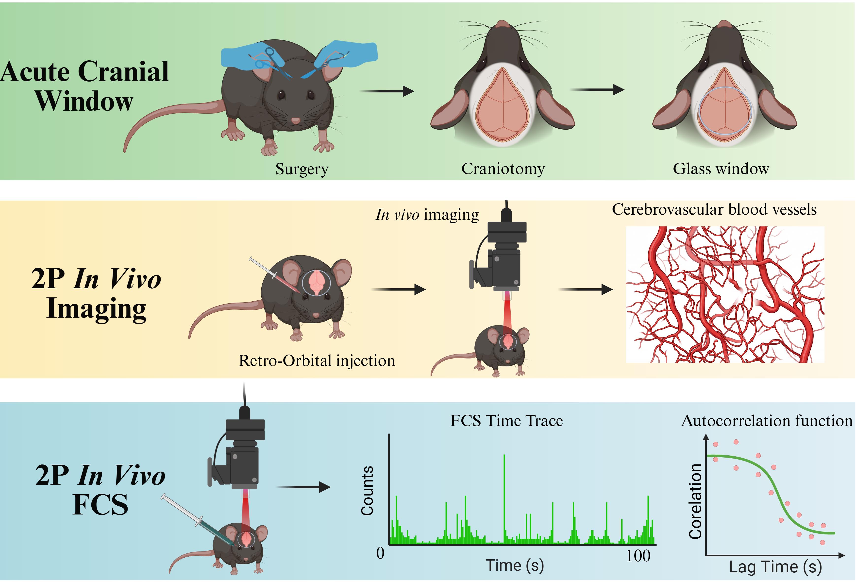
Figure 4. Experimental workflow for preparing cranial windows, two-photon (2P) in vivo imaging, and fluorescence correlation spectroscopy (FCS) to quantify cerebral blood flow
E3. FCS measurement
1. Go to the software’s FCS tab and select RhodGreen configuration from Methods.
2. Check the Positions mark on the FCS tab. This will allow you to mark the objective's position relative to specific blood vessels.
3. Go to the Positions tab under FCS and click on Position List. Now, go to Select, and you will see a marking sign appear on the screen.
4. Mark the middle of the capillaries and blood vessels you are interested in and add all of the positions of the FCS Positions list.
5. A common marking of blood vessels and capillaries after injecting Rhodamine B-dextran is shown in Figure 5.
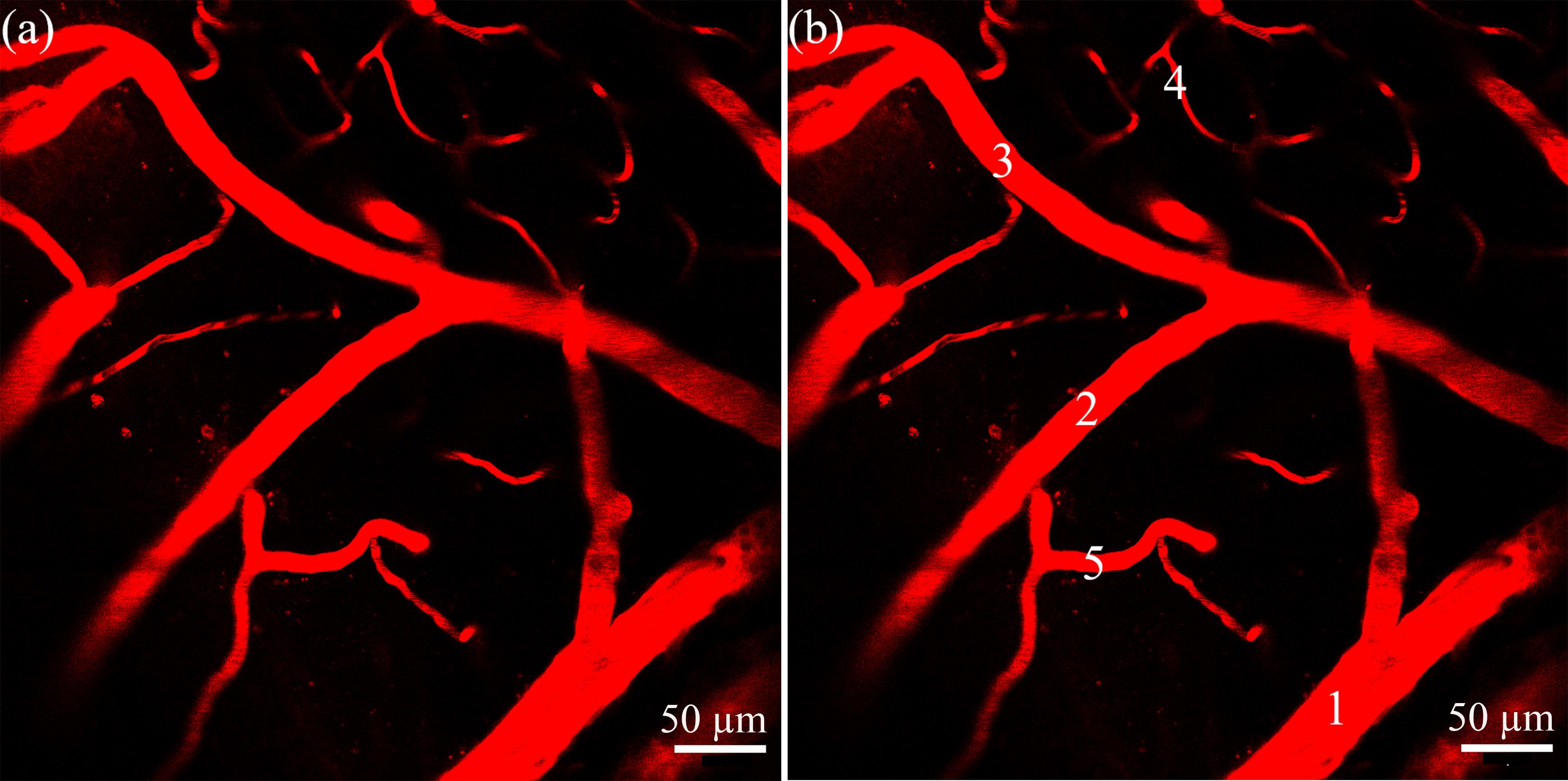
Figure 5. Two-photon image (2P) of (a) blood vessels after injecting Rhodamine B-dextran (70 kDa) and (b) marking positions (1–5) of the FCS probe in various blood vessels
6. Set the excitation wavelength to 920 nm for FCS measurement.
7. Adjust the laser power to approximately 20 mW.
8. Set the measurement time for 10 s with 10 repetitions.
9. Uncheck the Red Channel, since you will record fluorescence intensity fluctuations on the Green Channel.
10. Click Count Rate under FCS mode to observe the count of the background signals. Optimal count rates should typically remain below 200 kHz.
11. Now, start the experiment by clicking Start Experiment.
12. Save the file as a background FCS.
13. Prepare 30 μL of 0.1 mg/mL CF488-dextran (250 kDa) in 1× sterile PBS buffer.
14. Inject 30 μL of CF488-dextran dye retro-orbitally into the other eye of the mouse.
15. After the injection, repeat steps E3.10–11 to record the intensity fluctuations of CF488-dextran (Figure 4).
16. Save the files and the data to be analyzed to extract the average residence time and particle number under the confocal volume.
17. Repeat the measurement for more vessels or depths as necessary.
F. Post-imaging euthanasia
Following the imaging session, euthanize the mice by cervical dislocation or decapitation while remaining under anesthesia.
Data analysis
A. Calibration of the confocal lateral diameter
A1. Fitting FCS data to a flow model
The data will be analyzed in the same Zeiss software. The autocorrelation function of the FCS data will be fitted to the flow model to extract the average residence time in the confocal volume.
1. Open the data files in Zen Black software.
2. You will see the FCS time traces and autocorrelation function to the window.
3. Go to Fit from the list of icons. Now, choose a model for fitting. We will fit the autocorrelation function to the flow model.
4. There are a bunch of default models available. From the list, choose the Flow model.
5. The pure flow model is described by the following equation:
where G(τ) is the correlation between time trace signals, <N> is the average number of particles under the confocal volume, τf is the average residence time, and τf is the time lag.
6. Now click on Fit All to fit all autocorrelation functions of 10 measurements.
7. Look at the χ2 of the average measurement. If the χ2 of the average shows a value less than 1 × 10⁻⁵, it indicates a good fit.
8. Write the residence time in an Excel file. You will use this parameter for subsequent calculations.
A2. Calculations of the lateral diameter of confocal volume
1. The dimensions of the flow channel are 50 mm × 5mm × 0.2 mm. Multiply width and depth to find the cross-sectional area, which is 1 mm2.
2. Convert the unit of flow velocity from mL/min to mm3/s. Use the conversion factor of 1 mL = 1,000 mm3.
3. The flow velocity in mm/s can be found by dividing the velocity in mm3/s by the cross-sectional area of the flow channel.
4. Convert the flow velocity from mm/s to μm/μs by multiplying by 1,000.
5. In data analysis software, convert the residence time to its reciprocal.
6. Now, plot the reciprocal of flow residence time (μs-1) versus flow velocity (μm/μs) (Figure 1).
7. Fit the line to linear regression.
8. The slope of the fitting line is the lateral diameter (μs) of the confocal volume.
B. In vivo FCS data fitting
B1. Blood flow velocity calculations
1. Fit the in vivo FCS data with the same Zeiss software as described in section B3.
2. Extract the flow residence time for CF488-dextran in different blood vessels.
3. Now, divide the lateral diameter by the residence time of CF488-dextran in each blood vessel as follows:
4. Convert the blood flow velocity unit from μm/μs to mm/s.
B2. Nanocarrier concentration calculations
We will get the average number of particles in the confocal volume straight from the fitting function. However, we will fit the autocorrelation function by subtracting the background.
1. Open the background data files in Zeiss software.
2. Record the average count rate (kHz) of the in vivo background signals.
3. Now, open the in vivo data files.
4. Record the average count rate (kHz) of the in vivo FCS for each blood vessel and capillary.
5. You will fit these data to the flow model as before, by subtracting the background signals. Now, choose the flow model and click on Define in the software to define the background.
6. Check the Background check box.
7. Click on Settings under Background.
8. The background is defined as follows:
where Ib is the average background intensity, and It is the average intensity of the in vivo time traces.
9. Do a basic calculation for finding the value of B and put the value in the software.
10. Now, the autocorrelation function takes the following form:
11. As before, click on Fit All to fit all autocorrelation functions of 10 measurements.
12. Look at the χ2 of the average measurement.
13. After fitting, the software will give you the average amplitude particle number in the parameter table.
Validation of protocol
This protocol has been used and validated in the following research articles:
• Fu et al. [16]. In Vivo Single-Molecule Detection of Nanoparticles for Multiphoton Fluorescence Correlation Spectroscopy to Quantify Cerebral Blood Flow. Nano Letters (Figures 1–4, Supplemental Figures 1 and 3–6).
• Wang et al. [17]. DNA-AgNC Loaded Liposomes for Measuring Cerebral Blood Flow Using Two-Photon Fluorescence Correlation Spectroscopy (Figures 4 and 5, Supplemental Figures 16 and 17).
The optimized protocol has been further validated in the following research article, which demonstrated real-time measurements of nanocarrier concentration using multiphoton in vivo FCS:
• Wang et al. [18]. Real-Time In Vivo Detection of Nanocarrier Number and Velocity in the Cerebrovasculature Using Hot Band Absorption. Small (Figures 1 and 5, Supplemental Figures 8, 9, 12, 14, 15, and 18–20).
General notes and troubleshooting
General notes
1. The spectral crosstalk between blood vessel labeling and FCS tracking dye must be carefully optimized. In this protocol, Rhodamine B-dextran (70 kDa) and CF488-dextran (250 kDa) were used for vascular visualization and the FCS tracer, respectively. However, other dye combinations with adequate spectral separation may also work.
2. The two-photon excitation wavelengths of both dye combinations must be chosen carefully.
3. The excitation laser power must be optimized carefully to avoid the saturation of the detector.
4. The concentration of the FCS tracing dye must be optimized very carefully. The particle number should be roughly in the order of 1011 per milliliter.
5. To minimize motion artifacts, ensure that the cranial window is securely fixed, the mouse is properly anesthetized, and the head holder is firmly attached to the imaging stage.
6. Although this protocol was developed using a Zeiss LSM 880 multiphoton microscope with ZEN Black software, it can be adapted to other multiphoton microscopes equipped with photon-counting detectors and FCS acquisition modules.
Troubleshooting
Problem 1: Laser power instability.
Possible cause: It is very common for the femtosecond laser power output to fluctuate over time. This might happen due to insufficient warm-up of the femtosecond laser.
Solution: Allow the laser to warm up for at least 20–30 min before experiments. For each experiment, verify the power using a calibrated power meter.
Problem 2: Strong autofluorescence from the adhesive or dental cement.
Possible cause: Sometimes, strong autofluorescence arises from the glass window-fixing glue or dental cement. This might happen when glues or dental cement are placed in the cranial window after surgery.
Solution: Be especially careful when applying the adhesive for fixing the glass window. Use a fine needle tip to apply the glue.
Problem 3: Blood vessel position shifts after retro-orbital injection.
Possible cause: Often, after the second injection, the position of the blood vessel changes slightly due to the slight shift of the mouse's head position during injection.
Solution: After the second injection, verify the FCS probe position within the blood vessels by taking another 2P image and comparing it with the previously acquired images.
Problem 4: Overfitting or underfitting of FCS data.
Possible cause: It is very common for the FCS fitting data to give you something not practical due to overfitting or underfitting.
Solution: Always look at the FCS time traces to get an idea about the fitting parameters.
Supplementary information
The following supporting information can be downloaded here:
1. Table S1. Acute cranial window preparation guide.
Acknowledgments
Conceptualization: Sagar Pande; Investigation: Sagar Pande, Xiaojin Wang, and Xu Fu; Writing—Original Draft: Sagar Pande; Writing—Review & Editing, Funding acquisition, Supervision: Christopher I. Richards. Funding: NIH (GM138837 and GM138882).
The actual cranial window protocol was originally described and validated by Holtmaat et al. [22] in Nature Protocols (2009), DOI: 10.1038/nprot.2009.89. This protocol was used in [16–18]. The graphical illustrations were made with BioRender.com.
Competing interests
The authors declare no competing interests.
Ethical considerations
All animal experiments were performed in accordance with approved protocols and the guidelines of the Institutional Animal Care and Use Committee (IACUC) at the University of Kentucky.
References
- Iadecola, C. (2017). The Neurovascular Unit Coming of Age: A Journey through Neurovascular Coupling in Health and Disease. Neuron. 96(1): 17–42. https://doi.org/10.1016/j.neuron.2017.07.030
- Nielsen, R. B., Egefjord, L., Angleys, H., Mouridsen, K., Gejl, M., Møller, A., Brock, B., Brændgaard, H., Gottrup, H., Rungby, J., et al. (2017). Capillary dysfunction is associated with symptom severity and neurodegeneration in Alzheimer's disease. Alzheimers Dement. 13(10): 1143–1153. https://doi.org/10.1016/j.jalz.2017.02.007
- Iadecola, C. (2013). The Pathobiology of Vascular Dementia. Neuron. 80(4): 844–866. https://doi.org/10.1016/j.neuron.2013.10.008
- Starosolski, Z., Villamizar, C. A., Rendon, D., Paldino, M. J., Milewicz, D. M., Ghaghada, K. B. and Annapragada, A. V. (2015). Ultra High-Resolution In vivo Computed Tomography Imaging of Mouse Cerebrovasculature Using a Long Circulating Blood Pool Contrast Agent. Sci Rep. 5(1): e1038/srep10178. https://doi.org/10.1038/srep10178
- Pathak, A. P., Kim, E., Zhang, J. and Jones, M. V. (2011). Three-Dimensional Imaging of the Mouse Neurovasculature with Magnetic Resonance Microscopy. PLoS One. 6(7): e22643. https://doi.org/10.1371/journal.pone.0022643
- Denk, W., Strickler, J. H. and Webb, W. W. (1990). Two-Photon Laser Scanning Fluorescence Microscopy. Science. 248(4951): 73–76. https://doi.org/10.1126/science.2321027
- Zipfel, W. R., Williams, R. M. and Webb, W. W. (2003). Nonlinear magic: multiphoton microscopy in the biosciences. Nat Biotechnol. 21(11): 1369–1377. https://doi.org/10.1038/nbt899
- Dunn, A. K. (2011). Laser Speckle Contrast Imaging of Cerebral Blood Flow. Ann Biomed Eng. 40(2): 367–377. https://doi.org/10.1007/s10439-011-0469-0
- Calamante, F., Thomas, D. L., Pell, G. S., Wiersma, J. and Turner, R. (1999). Measuring Cerebral Blood Flow Using Magnetic Resonance Imaging Techniques. J Cerebr Blood F Met. 19(7): 701–735. https://doi.org/10.1097/00004647-199907000-00001
- Cenic, A., Nabavi, D. G., Craen, R. A., Gelb, A. W. and Lee, T.-Y. (1999). Dynamic CT measurement of cerebral blood flow: a validation study. Am J Neuroradiol. 20(1): 63–73.https://www.ajnr.org/content/20/1/63.long
- Zakharov, P., Völker, A., Wyss, M., Haiss, F., Calcinaghi, N., Zunzunegui, C., Buck, A., Scheffold, F. and Weber, B. (2009). Dynamic laser speckle imaging of cerebral blood flow. Opt Express. 17(16): 13904–13917. https://doi.org/10.1364/oe.17.013904
- Kisler, K., Lazic, D., Sweeney, M. D., Plunkett, S., El Khatib, M., Vinogradov, S. A., Boas, D. A., Sakadži´, S. and Zlokovic, B. V. (2018). In vivo imaging and analysis of cerebrovascular hemodynamic responses and tissue oxygenation in the mouse brain. Nat Protoc. 13(6): 1377–1402. https://doi.org/10.1038/nprot.2018.034
- Chaigneau, E., Roche, M. and Charpak, S. (2019). Unbiased Analysis Method for Measurement of Red Blood Cell Size and Velocity With Laser Scanning Microscopy. Front Neurosci. 13: e00644. https://doi.org/10.3389/fnins.2019.00644
- Kim, S. A., Heinze, K. G. and Schwille, P. (2007). Fluorescence correlation spectroscopy in living cells. Nat Methods. 4(11): 963–973. https://doi.org/10.1038/nmeth1104
- Schmitt, S., Huppertsberg, A., Klefenz, A., Kaps, L., Mailänder, V., Schuppan, D., Butt, H. J., Nuhn, L. and Koynov, K. (2022). Fluorescence Correlation Spectroscopy Monitors the Fate of Degradable Nanocarriers in the Blood Stream. Biomacromolecules. 23(3): 1065–1074. https://doi.org/10.1021/acs.biomac.1c01407
- Fu, X., Sompol, P., Brandon, J. A., Norris, C. M., Wilkop, T., Johnson, L. A. and Richards, C. I. (2020). In Vivo Single-Molecule Detection of Nanoparticles for Multiphoton Fluorescence Correlation Spectroscopy to Quantify Cerebral Blood Flow. Nano Lett. 20(8): 6135–6141. https://doi.org/10.1021/acs.nanolett.0c02280
- Wang, X., Liisberg, M. B., Nolt, G. L., Fu, X., Cerretani, C., Li, L., Johnson, L. A., Vosch, T. and Richards, C. I. (2023). DNA-AgNC Loaded Liposomes for Measuring Cerebral Blood Flow Using Two-Photon Fluorescence Correlation Spectroscopy. ACS Nano. 17(13): 12862–12874. https://doi.org/10.1021/acsnano.3c04489
- Wang, X., Liisberg, M. B., Rück, V., Pande, S., Nolt, G. L., Li, L., Yin, Q., Harvey, B. T., Nagel, J., Fu, X., et al. (2026). Real-Time In Vivo Detection of Nanocarrier Number and Velocity in the Cerebrovasculature Using Hot Band Absorption. Small. 22(17): e202508822. https://doi.org/10.1002/smll.202508822
- Ricard, C., Arroyo, E. D., He, C. X., Portera-Cailliau, C., Lepousez, G., Canepari, M. and Fiole, D. (2018). Two-photon probes for in vivo multicolor microscopy of the structure and signals of brain cells. Brain Struct Funct. 223(7): 3011–3043. https://doi.org/10.1007/s00429-018-1678-1
- Xu, C. and Webb, W. W. (1996). Measurement of two-photon excitation cross sections of molecular fluorophores with data from 690 to 1050 nm. J Opt Soc Am B. 13(3): 481–491. https://doi.org/10.1364/josab.13.000481
- Xu, C. and Webb, W. W. (2002). Multiphoton Excitation of Molecular Fluorophores and Nonlinear Laser Microscopy. In: Topics in fluorescence spectroscopy: volume 5: nonlinear and two-photon-induced fluorescence. Springer, 471–540. https://doi.org/10.1007/0-306-47070-5_11
- Holtmaat, A., Bonhoeffer, T., Chow, D. K., Chuckowree, J., De Paola, V., Hofer, S. B., Hübener, M., Keck, T., Knott, G., Lee, W. C., et al. (2009). Long-term, high-resolution imaging in the mouse neocortex through a chronic cranial window. Nat Protoc. 4(8): 1128–1144. https://doi.org/10.1038/nprot.2009.89
Article Information
Publication history
Received: Mar 13, 2026
Accepted: May 6, 2026
Available online: May 27, 2026
Published: Jul 5, 2026
Copyright
© 2026 The Author(s); This is an open access article under the CC BY-NC license (https://creativecommons.org/licenses/by-nc/4.0/).
How to cite
Pande, S., Wang, X., Fu, X., Prathapasinghe, H. and Richards, C. I. (2026). Protocol for In Vivo Two-Photon FCS to Measure Nanocarrier Number and Flow Velocity in Mouse Cerebral Microvasculature. Bio-protocol 16(13): e5717. DOI: 10.21769/BioProtoc.5717.

 Download Citation in RIS Format
Category
Neuroscience > Neuroanatomy and circuitry > Fluorescence imaging
Biophysics > Microscopy > Two-photon laser scanning microscopy
Biological Engineering > Biomedical engineering > Drug Delivery
Do you have any questions about this protocol?
Post your question to gather feedback from the community. We will also invite the authors of this article to respond.
 Post a Question


