


- Protocols

- Articles and Issues
- For Authors
- About
- Become a Reviewer


Measuring Electrophysiological Activity in Acute Brain Slices, Spheroids, and Organoids Using 3D High-Density Multielectrode Arrays

(*Contributed equally to this work, ΘContributed equally to this work, §Technical contact: ivan.verduci@3brain.com) Published: Vol 16, Iss 11, Jun 5, 2026 DOI: 10.21769/BioProtoc.5708 Views: 1228
Reviewed by: Elena A. OstrakhovitchXiaochen SunMario Valentino
 PDF
PDF  Ask a question
Original research article
The authors used this protocol in:

Sep 2025
Advertisement




Protocol Collections
Comprehensive collections of detailed, peer-reviewed protocols focusing on specific topics




Abstract
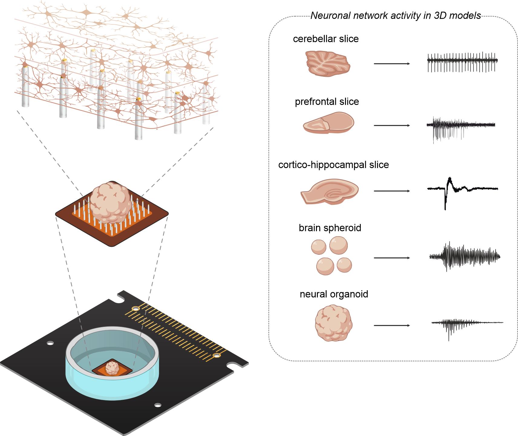
Animal and human stem cell–derived three-dimensional models to study physio-pathological brain functioning are becoming a gold standard for in vitro electrophysiology, as they enable the recapitulation of complex network properties by accounting for spatial architectural features that better reflect in vivo conditions than simpler 2D models. Standard planar multielectrode arrays (MEAs), typically providing tens of recording electrodes, are commonly used to record activity from 2D neuronal cultures. However, when adapted for use with 3D models, planar 2D MEAs showed limited effectiveness. The main issues are limited specimen adhesion to the chip, a low number of sensing elements, inability to retrieve signals from within the tissue, and reduced perfusion and vitality of the tissue in contact with sensors. To overcome these limitations, a new generation of microchip-based 3D high-density MEAs (3D HD-MEA) has been developed and validated in recent years. This technological advancement has improved the sensing capabilities and the vitality of 3D models, providing a tool tailored to maximize their potential. Here, we present an optimized protocol for neural network activity recordings in 3D models (including acute slices, brain spheroids, and organoids) from various brain regions using 3D HD-MEAs. First, we summarize the critical steps for 1) obtaining viable acute slices from the mouse cerebellum, cortico-hippocampal circuit, and prefrontal cortex, 2) establishing efficient coupling of the slices with the chip, and 3) performing recordings and analyses. We then describe the main procedures required to obtain human and animal brain spheroids and neural organoids, as well as standardized routines to perform effective recordings and analyses. For each section, we highlight the crucial steps, identify tips for specific applications, and propose troubleshooting procedures. For example, the same type of preparation (e.g., acute slices) requires different adjustments when working with different brain areas. The specific information provided here is intended to assist researchers in their daily efforts to obtain efficient and reproducible functional recordings from 3D models by using the cutting-edge technique of 3D HD-MEA.
Key features
• Comprehensive all-in-one guide covering the complete workflow for acquiring electrophysiological data from brain slices, neural region-specific organoids, and brain spheroids.
• Intuitive, step-by-step protocol for brain slice preparation, enriched with practical tips and expert recommendations to ensure high-quality tissue viability.
• Detailed instructions for optimal use of 3D HD-MEA technology, including proper handling of the sample holder for recordings from brain slices, neural organoids, and spheroids.
• In-depth guidance on BrainWave6 software, providing clear procedures for data acquisition, signal detection, and advanced electrophysiological analysis across all sample types.
Keywords: 3D high-density multielectrode array Acute slices
Brain spheroids
Neural organoids
Electrophysiological recordings
Electrophysiological data analysis
Acute electrophysiological measurements
Acute slices
Brain spheroids
Neural organoids
Electrophysiological recordings
Electrophysiological data analysis
Acute electrophysiological measurements
Graphical overview
Background
To date, 3D biological models with varying complexity are used to recapitulate the physiological features of animal and human nervous system circuitry, allowing for the study of physio-pathological brain activity [1–3]. Recent advances in stem cell technology have introduced the possibility of producing region-specific neural organoids from human-induced pluripotent stem cells (hiPSCs). Animal models offer fully mature, structurally accurate brain architectures, which are crucial for examining circuit functions and understanding how diseases affect the neuronal electrical activity [4,5]. In contrast, human-derived neural organoids and the simpler brain spheroids, which can be derived from human neural progenitors but lack the structural and regional organization typical of organoids, can replicate unique human features, thereby reducing challenges in translating research findings to humans [6–8]. Furthermore, as these models can be maintained in culture for extended periods (up to years), they provide opportunities for detailed neurodevelopmental studies. Additionally, neural organoids can generate diverse patterned cell types, such as cortical, thalamic, and spinal cord cells, and achieve greater functional maturation than 2D cultures [9,10], though not equivalent to adult human brains. This enables the study of complex, in vivo–like brain network formation [11–15].
Several techniques exist to study neuronal activity in 3D models, including patch-clamp recordings, calcium imaging, and multielectrode arrays (MEA). In particular, MEAs represent the ideal technique for characterizing the electrophysiological activity of neuronal networks in these models, enabling simultaneous non-invasive recordings from multiple locations within the network, maintaining single-cell resolution, and providing excellent spatial resolution with the recent introduction of microchip-based high-density MEAs (HD-MEAs) [16–18]. For these reasons, HD-MEA devices are already in use with several 3D models, such as acute slices [18–21] and organoids [2,22–24]. However, planar probes commonly used for electrophysiological recordings are insufficient to exploit the complex network architecture that provides the main advantage of using these models. For instance, the chip is in contact only with the surface of the sample, interfacing the electrodes solely with the outermost cell layers. As a result, it fails to capture the activity occurring within the deeper, denser, and more interconnected layers. Even more critical, signals may be dampened by the presence of a dead cell layer in acute slices or by scaffolding materials, such as Matrigel, that are required to embed organoids in some protocols [25–27]. Another important aspect concerns vitality, which is compromised when the tissue is pushed against the chip. This dramatically reduces the recorded surface supply of oxygen and nutrients required to sustain the sample's viability. To fully harness the potential of HD-MEA in combination with 3D tissues, a recent technological breakthrough is represented by the integration of 3D electrodes that can penetrate the tissue and record neuronal activity from inner layers. In addition, these new devices have been equipped with a microstructure at the base of the 3D electrodes that forms microchannels below the tissue, thereby enhancing viability and accelerating pharmacological testing [28].
This methodology is well-suited for detailed investigations of neural network dynamics within 3D biological models, opening new opportunities to understand the relationship between structure and function in preparations, such as brain slices and organoids, that display a significant circuit architecture. This makes the technique ideal for a range of applications across multiple areas of neuroscience, including neurodevelopment, neuropharmacology, and neuropathology. For example, the technique's sensitivity would allow the uncovering of subtle modifications in neuronal firing and network dynamics in disease models with altered neuronal excitability and anatomical connectivity. This aspect is particularly relevant for characterizing organoids' functional network connectivity and its modification during development and in pathological models. Moreover, another promising field of application is certainly the testing of neuroprotective or neurotoxic compounds, which will benefit from the high efficiency of activity recordings from 3D models that more closely recapitulate in vivo conditions and can be maintained in more physiological environments than 2D models. Overall, this methodology provides a versatile platform for researchers working with diverse 3D neural models to investigate physiological mechanisms and disease-related dysfunctions with high reproducibility.
Indeed, the introduction of this new generation of 3D HD-MEA devices addresses the limitations that previously hindered the effectiveness of recordings by using planar devices. However, their unique surface, made up of micropillars approximately 90 μm tall, arranged in a 64 × 64 matrix with an electrode pitch of 60 μm, combined with the complexity of 3D biological models, requires specific adjustments to the experimental preparation and the application of this technology, which are crucial to ensure high-quality recordings. This protocol offers a comprehensive overview of preparing, mounting, recording, and analyzing acute 3D HD-MEA experiments from various 3D models: cerebellar, prefrontal cortex, and cortico-hippocampal acute slices, brain spheroids, and cortical and spinal cord organoids. For clarity, the paper is organized into two independent sections, one for slices and the other for spheroids and organoids. The protocols reported here are intended to enhance researchers’ ability to record functional activity from different types of 3D biological samples.
Part I: Acute brain slices
Materials and reagents
Reagents
1. Sodium chloride (NaCl) (Sigma-Aldrich, CAS-number: 7647-14-5)
2. Potassium dihydrogen phosphate (KH2PO4) (Sigma-Aldrich, CAS-number: 7778-77-0)
3. Potassium chloride (KCl) (Sigma-Aldrich, CAS-number: 7447-40-7)
4. Magnesium sulfate heptahydrate (MgSO4·7H2O) (Sigma-Aldrich, CAS-number: 10034-99-8)
5. Calcium chloride dihydrate (CaCl2·2H2O) (Sigma-Aldrich, CAS-number: 10035-04-8)
6. Sodium phosphate (NaHPO4) (Sigma-Aldrich, CAS-number: 7558-79-4)
7. Sodium bicarbonate (NaHCO3) (Sigma-Aldrich, CAS-number: 144-55-8)
8. D-(+)-glucose (Sigma-Aldrich, CAS-number: 50-99-7)
Solutions
1. Krebs solution for cerebellar slices [29] (see Recipes)
2. Modified artificial cerebrospinal fluid (mACSF) for prefrontal cortex slices [30] (see Recipes)
3. Krebs high-potassium and high-calcium for cortico-hippocampal slices (see Recipes)
Recipes
1. Krebs solution for cerebellar slices
| Reagent | Concentration (mM) |
|---|---|
| NaCl | 120 |
| KH2PO4 | 1.18 |
| KCl | 2 |
| MgSO4·7H2O | 1.2 |
| CaCl2·2H2O | 2 |
| NaHCO3 | 26 |
| Glucose | 11 |
Adjust the solution to the desired volume with double-distilled water. pH of 7.4 is maintained when equilibrated with 95% O2, 5% CO2. Expected osmolarity: 300 ± 10 mOsm.
2. Modified ACSF solution for prefrontal cortex slices
| Reagent | Concentration (mM) |
|---|---|
| NaCl | 124 |
| KCl | 3.5 |
| NaHPO4* | 1 |
| CaCl2·2H2O | 1.25 |
| NaHCO3 | 26 |
| Glucose | 10 |
*After this step, add carbogen gas (95% O2, 5% CO2) to the solution for 30 min before adding calcium chloride to avoid salt precipitation.
Adjust the solution to the desired volume with double-distilled water. pH of 7.4 is maintained when equilibrated with 95% O2, 5% CO2. Expected osmolarity: 300 ± 10 mOsm.
3. Krebs high-potassium and high-calcium for cortico-hippocampal slices
| Reagent | Concentration (mM) |
|---|---|
| NaCl | 115.18 |
| KH2PO4 | 1.18 |
| KCl* | 6.82 |
| CaCl2·2H2O | 4 |
| NaHCO3 | 26 |
| Glucose | 11 |
*After this step, add carbogen gas (95% O2, 5% CO2) to the solution for 30 min before adding calcium chloride to avoid salt precipitation.
Adjust the solution to the desired volume with double-distilled water. pH of 7.4 is maintained when equilibrated with 95% O2, 5% CO2. Expected osmolarity: 300 ± 10 mOsm.
Laboratory supplies
1. Whatman® qualitative filter paper, Grade 1 (Sigma-Aldrich, catalog number: 1001-090)
2. Pasteur pipette 7 mL (Sigma-Aldrich, catalog number: BR747770)
3. Large weighing dishes (Sigma-Aldrich, catalog number: Z154881)
4. Small/medium weighing boats (Sigma-Aldrich, catalog number: W3001)
5. Extran® MA 02 (Sigma-Aldrich, catalog number: 1.07553)
6. Ethanol, pure (Sigma-Aldrich, catalog number: 32205-M)
7. Nitrile extra light gloves (VWR, Avantor, catalog number: 112-4195)
8. Plastic bag
9. Cyanoacrylate glue
10. Double-distilled water
Equipment
1. 500 mL Pyrex beaker
2. 250 mL Pyrex beaker
3. 50 mL beaker
4. Osmometer (Gonotec®, OsmomatTM 030) and calibration standard (Gonotec®, catalog number: 30.9.0500)
5. Vibroslicer (Leica BIOSYSTEMS, catalog number: VT1200S)
6. Vibroslicer chamber
7. Vibroslicer cutting plate
8. Glass Petri dish
9. Large scissors
10. Fine scissors
11. Fine tweezers
12. Semi-curved spatulas
13. Halved razor blade
14. Small flat-blade scalpel (No. 10)
15. Carbon steel scalpel (F.S.T., catalog number: 103115-12)
16. BioCAM (3Brain, DupleX)
17. 3D HD-MEA (3Brain, CorePlateTM 3D 1W 38-60-90)
18. Sample holder frame (3Brain, Sample Holder 2, Frame)
19. Sample holder insert (3Brain, Sample Holder 2, 1000 μN)
20. Sample holder silicone net (3Brain, Sample Holder 2, Silicone Net)
21. Sample holder handling tool (3Brain, Sample Holder 2, Handling tool)
22. Gas inlet/outlet tubes (Cole, Parmer, catalog numbers: 072-031-1, 072-063-1 C-FLEX)
23. Tubes (IsmatecTM, TYGON LMT, 55, ID 0.64 mm, WALL 0.90 mm)
24. Peristaltic pump (IsmatecTM, MS-4/12 Reglo Digital Pump)
Software and datasets
1. BrainWave6 (3Brain), requires a license
2. IC Capture (The Imaging Source, Version 2.4)
3. NEUROPulse (10.5281/zenodo.18196676)
Procedure
A. Recovery beaker setup
1. Prepare a 250 mL Pyrex beaker, a cut syringe, and a ring acrylic plate with legs covered by a net fabric (Figure 1A).
Note: The net fabric is not glued to the ring plexiglass plate; instead, it is blocked by a small plexiglass ring inserted in the plate, since the glue can be toxic to slices. Avoid colored net fabric to limit any leaching of chemical substances in the recovery solution.
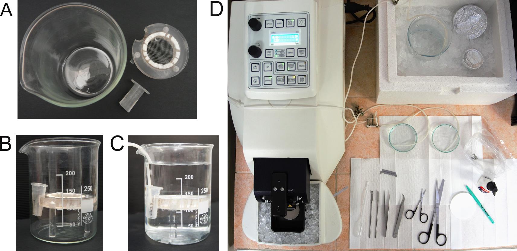
Figure 1. Recovery beaker and cutting bench setup. (A, B) Components of the recovery beaker and proper mounting. (C) Recovery beaker filled with Krebs solution. (D) Setup with all the necessary equipment for the procedure.
2. Insert the acrylic plate in the beaker and secure it by placing the cut syringe between the beaker wall and the acrylic plate (Figure 1B).
3. Fill the recovery beaker with 220 mL of Krebs solution (see Recipes) at room temperature and bubble the solution continuously with a 95% O2, 5% CO2 gas mixture, inserting the gas inlet tube in the cutting syringe (Figure 1C). Remove bubbles under the net using a Pasteur pipette.
Notes:
1. The Krebs solution should fill 3/4 of the recovery beaker to ensure proper perfusion of the slices.
2. Bubbles under the net do not allow proper perfusion of the slices.
Critical: When adding the Krebs solution, avoid any large bubble buildup beneath the entire underlying surface of the net.
Critical: Do not put the gas inlet tube too deep in the cut syringe to avoid the continuous formation of bubbles under the net.
B. Cutting bench setup
1. Transfer 300 mL of Krebs solution into a 500 mL Pyrex beaker. Place the beaker in a polystyrene ice box filled with ice. Bubble the solution continuously with a 95% O2, 5% CO2 gas mixture for at least 30 min before starting the cutting procedure to ensure adequate cooling (2–4 °C) and pH balance (pH 7.4).
2. Wrap the vibroslicer chamber, the vibroslicer cutting plate, three Petri dishes, and one 50 mL beaker in aluminum foil to prevent direct contact with ice crystals, and place them in the freezer.
3. Place the instruments required for the cutting procedure on the slicing bench adjacent to the vibroslicer in the order of use. This includes one large scissors, one fine scissors, two fine tweezers, two semi-curved spatulas, one halved razor blade, one Pasteur pipette, one sheet of Whatman grade 1 filter paper, a carbon steel scalpel, and a tube of cyanoacrylate glue. Keep a small plastic bag on the right side to collect the animal remains.
4. Immediately before starting the brain extraction, prepare the vibroslicer. Remove the vibroslicer chamber from the freezer, insert it in its support, and place crushed ice in the tray surrounding the chamber.
5. Remove the vibroslicer cutting plate and three Petri dishes from the freezer. Place two dishes on the bench and fill with ice-cold, carbogenated Krebs solution. Maintain continuous bubbling using the appropriate gas inlet tube. Leave the remaining dish in the polystyrene ice box for later use (see step C13) (Figure 1D).
Critical: Perform steps B4–5 only immediately before starting the slicing procedure. Keeping all components ice-cold is essential to preserving tissue viability and ensuring optimal slicing quality.
C. Brain extraction
1. Anesthetize the mouse using isoflurane, sevoflurane, or halothane, as appropriate for your experiment.
Caution: Perform this step under a fume hood or in a well-ventilated area to avoid inhalation of vapors and ensure operator safety.
2. Verify the depth of anesthesia by checking for the absence of nociceptive reflexes. Pinch the hind paw or gently compress the tail using tweezers and confirm that no withdrawal or reflexive movement occurs.
3. Decapitate the mouse rapidly with large surgical scissors. Perform the cut in a single motion to minimize stress.
4. Retract the skin anteriorly toward the snout to fully expose the skull.
Note: Use fine scissors to remove residuals of connective tissue covering the skull to allow proper retraction of the scalp.
5. Place the exposed skull in a Petri dish containing ice-cold, carbogenated Krebs solution to cool the tissue.
Note: Cooling reduces enzymatic activity and preserves tissue integrity before dissection.
6. Insert small scissors into the foramen magnum, keeping the blades parallel to both the bench and the base of the skull. Advance rostrally with a low, horizontal trajectory, cutting along one side of the skull toward the snout until reaching the frontal suture.
Critical: Maintain the skull in a position parallel to the bench to ensure a controlled and safe cut.
Critical: Keep the scissors flat against the skull and close to its base. Do not angle them upward toward the brain to avoid damaging underlying brain tissue.
7. After cutting the first lateral side, advance the scissors rostrally along the curvature of the cranial bone, gradually moving up the blades as you approach the anterior skull. Continue cutting upward until the nasal bone is reached and incised. Follow the curvature of the skull downward along the opposite lateral side to complete the dorsal skull opening.
Critical: Cut only the cranial bone and avoid contact with neural tissue. Ascend gently only in the final segment to complete the opening without injuring brain tissue.
8. Insert a semi-curved spatula laterally between the inner surface of the skull and the brain. Gently introduce a small amount of air to loosen the meninges and facilitate detachment of the brain.
Critical: Do not contact the brain tissue with a spatula to avoid damage.
9. Rasp the lateral edges of the opened skull with fine tweezers and elevate the bone carefully without applying traction to the brain. Maintain slow, controlled motion to prevent tissue damage.
10. Cut any remaining neural connections if necessary, using fine scissors or the spatula. Sever the optic nerves ventrally and the cranial nerves caudally using minimal and controlled incisions to free the brain while preserving tissue integrity.
11. Lift the brain gently out of the cranial cavity once all attachments are released.
12. Transfer the brain immediately into a Petri dish containing ice-cold, carbogenated Krebs solution to maintain tissue viability.
13. Retrieve the Petri dish from the polystyrene box filled with ice. Remove the aluminum foil and place the dish inverted on the setup.
14. Place a Whatman filter paper over the inverted Petri dish and apply cold, carbogenated Krebs solution dropwise using a Pasteur pipette to wet the filter thoroughly.
15. At this stage, the brain and cerebellum are fully exposed and free of residual cranial attachments and ready for subsequent procedures, including dissection of the cerebellar vermis (Section D), the prefrontal region (Section E), and the cortico-hippocampal region (Section F).
D. Cerebellar vermis dissection and slice preparation
1. Using two semi-curved spatulas, transfer the isolated brain onto the wet filter paper (Figure 2A).
2. Using a halved razor blade, make a straight incision in the fissure between the cerebrum and the cerebellum (Figure 2B).
3. Carefully remove the cerebrum with a semi-curved spatula to isolate the cerebellum (Figure 2C).
4. Cut one cerebellar hemisphere using a halved razor blade, keeping the cut straight and leaving a margin of tissue adjacent to the vermis to prevent its accidental removal or damage during hemisphere excision. Remove the excised hemisphere with a semi-curved spatula. Repeat the same procedure to remove the contralateral hemisphere (Figure 2D–F).
Notes:
1. The first hemisphere should be cut as straight as possible, as the presence of both hemispheres helps stabilize the specimen and maintain a level cut. When cutting the second hemisphere, the absence of the first reduces stability, making a straight incision more difficult. Record which side was cut first, as it provides the flattest surface to be glued on the vibroslicer cutting plate (see step D9).
2. Maintaining a small pontine fragment attached to the cerebellum prevents tissue movement and deformation when the specimen is glued onto the vibroslicer cutting plate. Remove only the portion that has detached spontaneously by gently trimming it with a halved razor blade.
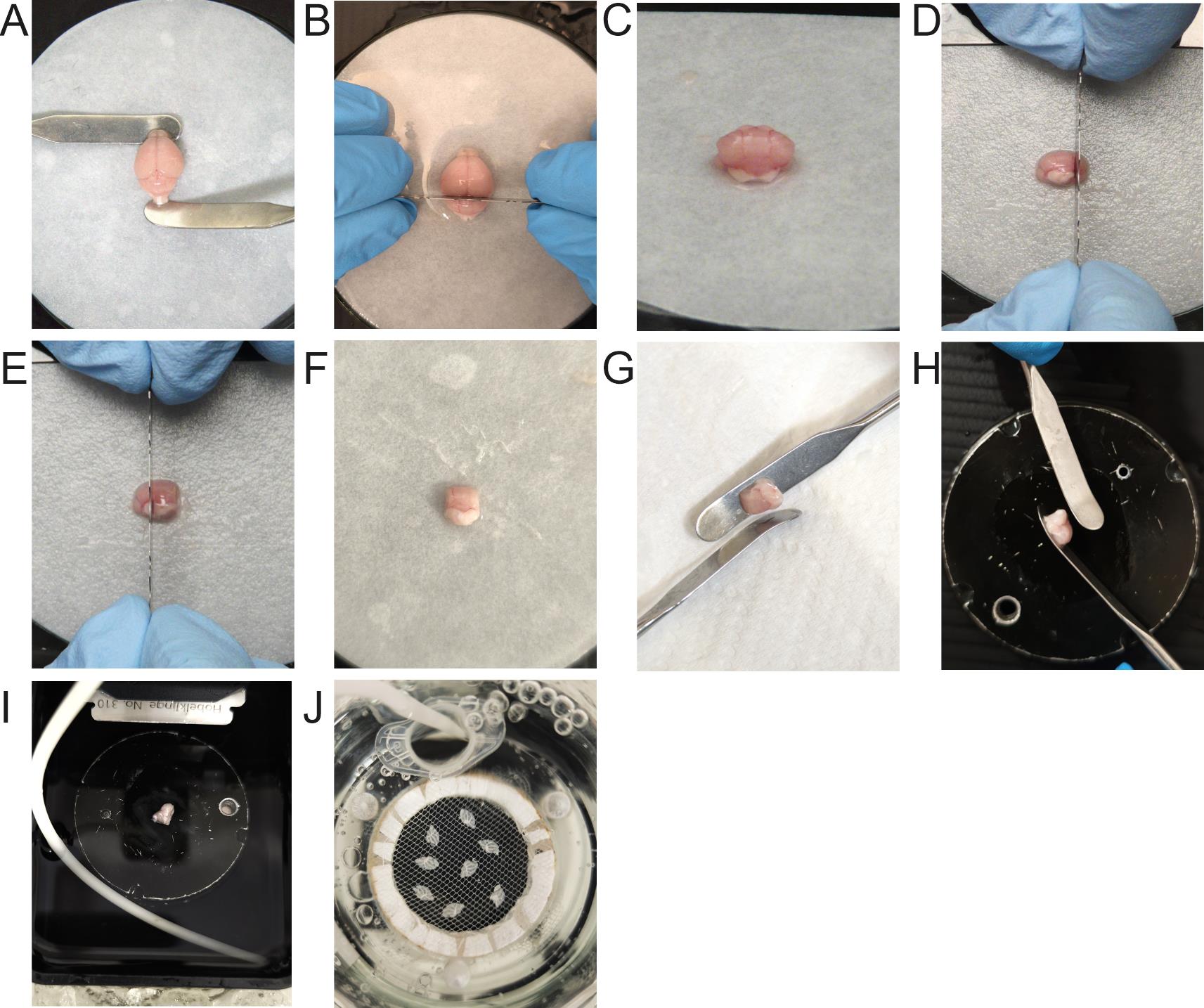
Figure 2. Dissection of the cerebellar vermis and slice preparation. (A) Isolated brain. (B–F) Steps of the cutting procedure to isolate the cerebellar vermis. (G, H) Removal of excess solution from the sample and attachment to the plate. (I) Sectioning of the tissue. (J) Recovery beaker containing cerebellar vermis slices.
5. Transfer the isolated cerebellar vermis into a Petri dish containing ice-cold, carbogenated Krebs solution.
6. Retrieve the vibroslicer cutting plate from the polystyrene box filled with ice, remove the aluminum foil, and apply cyanoacrylate glue to the plate using a fine brush. Spread the glue first along one direction of the plate, then in the perpendicular direction to ensure even distribution across the surface.
Critical: Avoid applying excessive glue and do not overbrush, as this may result in uneven coating with areas of too much or too little adhesive.
7. Using a semi-curved spatula, transfer the cerebellar vermis onto the glued plate, positioning the side corresponding to the first hemisphere cut against the plate (facing away from you) and the side corresponding to the second cut facing toward you. Then, place a second spatula against the side corresponding to the first cut to stabilize the vermis and prevent tilting or slipping during placement.
8. Carefully bring the spatulas with the vermis toward a piece of absorbent paper so that excess liquid is drawn away by capillary action (Figure 2G).
Critical: Proper removal of excess liquid is crucial. Residual fluid can prevent optimal adhesion to the glue, compromising subsequent slicing.
9. Rotate the spatula holding the vermis by 90° so that the side corresponding to the first cut is now facing downward. Gently slide down the vermis onto the glue using the other spatula, allowing the specimen to adhere properly to the glue (Figure 2H). Once the first cut side is secured, apply gentle pressure on the other side with the spatula to ensure complete adhesion of the vermis.
10. Immediately place the plate with the adhered cerebellar vermis into the slicing chamber, orienting the tissue with the pons facing toward the operator and the cerebellar cortex facing the back of the vibroslicer.
Note: This orientation prevents the blade from encountering the pons first, which could create mechanical resistance and cause tissue displacement or tearing during sectioning.
11. Gently pour the ice-cold Krebs solution from a corner of the slicing chamber, rather than directly onto the glued brain, until the chamber is almost filled (approximately 120 mL of Krebs solution) and insert a gas inlet tube to maintain continuous carbogenation during the entire procedure (Figure 2I).
Note: Direct flow onto the specimen may dislodge it from the plate and compromise the slicing procedure.
12. Add cold tap water (previously stored in the refrigerator) into the outer tray containing ice to create a chilled mixture that supports low-temperature slicing.
Notes:
1. Do not add this water earlier, as it may cause excessive melting of the ice and reduce the cooling efficiency.
2. Add additional crushed ice into the outer tray if excessive melting occurs.
13. Insert a halved razor blade into the vibroslicer guide. Adjust the blade so that the white alignment mark on the left is fully visible while the right mark is just appearing. Secure the blade using a dedicated screwdriver inserted from the side.
14. Immerse the blade in the solution using the vibroslicer panel control. Set the cutting window to define the start and end points of slicing.
Note: Leave a small margin on each side to ensure the entire vermis is within the cutting window and no regions that need to be sliced are missed.
15. Set the vibroslicer speed to 0.06 mm/s and slice thickness to 220 μm for the sagittal section of the cerebellar vermis.
Note: These settings optimize slicing by balancing speed and precision, allowing rapid sectioning without damaging the tissue, while maintaining an appropriate thickness to preserve cerebellar cytoarchitecture and ensure reliable electrophysiological recordings.
16. Start the slicing procedure.
17. The initial slices will include residual portions of the cerebellar hemispheres. As slicing progresses, the vermis will begin to appear.
Note: The vermis can be distinguished from the hemispheres by the pattern of mossy fibers: in the vermis, mossy fibers enter and branch to form the characteristic ten lobules, whereas in the cerebellar hemispheres, fewer lobules are formed, and the mossy fiber bundles are thicker at the base.
18. During slicing, maintain each slice flat against the blade by applying gentle pressure on the overlying solution using a modified Pasteur pipette with the tip removed. This ensures consistent contact with the blade and prevents folding or displacement.
Note: If the final portion of a slice does not separate easily, use a carbon steel scalpel to carefully sever any remaining filaments or meningeal tissue that may impede complete detachment.
19. Transfer each vermis slice into a 50 mL beaker, previously stored in the freezer, containing ice-cold, carbogenated Krebs solution using a Pasteur pipette.
Note: This serves as a temporary holding step before transferring all slices to the recovery beaker (see section A).
20. Repeat the procedure until all cerebellar slices are obtained and transferred to the recovery beaker containing carbogenated Krebs solution for at least 1 h at room temperature.
Note: Typically, 7–9 sagittal slices of the cerebellar vermis are obtained at a thickness of 220 μm (Figure 2J).
21. The slices are then ready for 3D HD-MEA recordings.
Critical: Brain slices are fresh and delicate samples whose viability is known to decrease within hours. For cerebellar slices, perform your recording within 5–7 h.
E. Prefrontal region dissection and slice preparation
1. Using two semi-curved spatulas, transfer the isolated brain onto the wet filter paper (Figure 3A).
2. Use a halved razor blade to make a straight incision in the fissure between the cerebrum and cerebellum (Figure 3B).
3. Carefully remove the cerebellum with a semi-curved spatula to isolate the cerebrum.
Critical: Keep the olfactory bulbs intact throughout the entire procedure, as the prefrontal region lies immediately posterior to them. Damaging or detaching the bulbs may compromise the prefrontal region.
4. Make an additional cut at the posterior base of the cerebrum to isolate the frontal portion containing the prefrontal region (Figure 3C, D).
Note: Removing a portion of the posterior brain increases the adhesion area, helping stabilize the specimen to the glue.
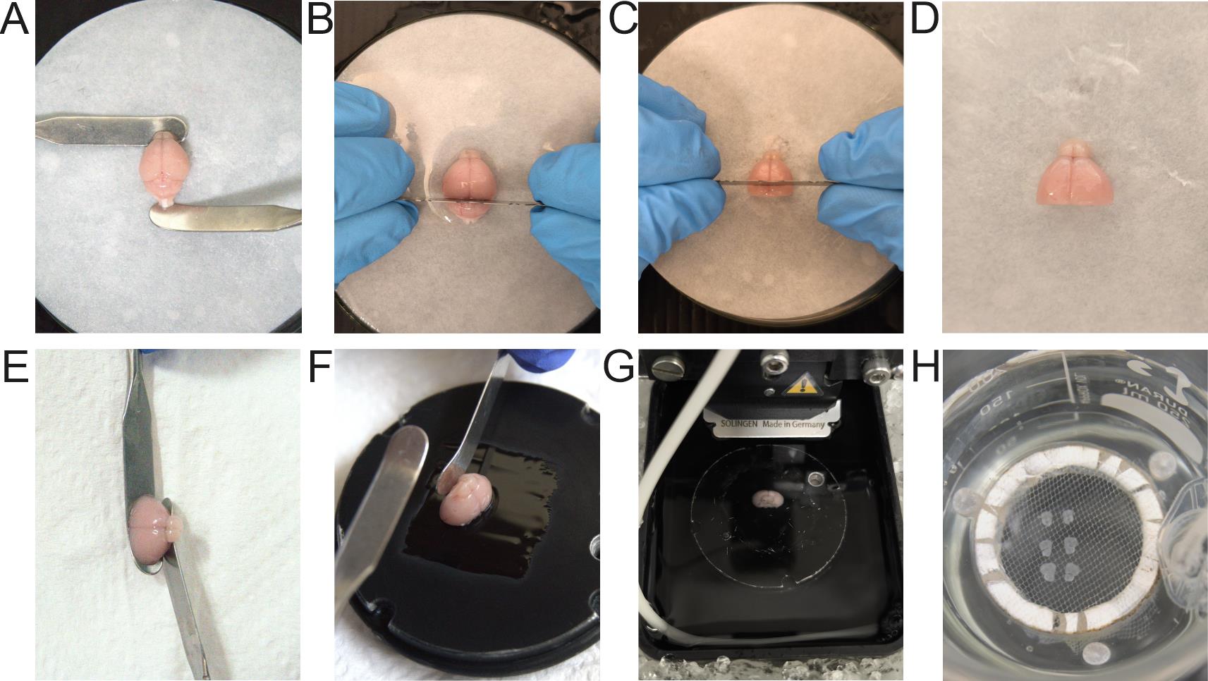
Figure 3. Dissection of the prefrontal region and slice preparation. (A) Isolated brain. (B–D) Steps of the cutting procedure to isolate the prefrontal region. (E, F) Removal of excess solution from the sample and attachment to the plate. (G) Sectioning of the tissue. (H) Recovery beaker containing prefrontal slices.
5. Transfer the isolated frontal portion into a Petri dish containing ice-cold, carbogenated Krebs solution.
6. Retrieve the vibroslicer cutting plate from the polystyrene box filled with ice, remove the aluminum foil, and apply cyanoacrylate glue to the plate using a fine brush. Spread the glue first along one direction of the plate, then in the perpendicular direction to ensure even distribution across the surface.
Critical: Avoid applying excessive glue and do not overbrush, as this may result in uneven coating with areas of too much or too little adhesive.
7. Place the cut frontal brain portion onto a semi-curved spatula with the base of the cerebrum on the spatula and the hemispheres facing upward. Then, position the other spatula against the ventral side of the cerebrum. This spatula stabilizes the specimen, preventing tilting or slipping while removing the specimen from the Petri dish.
8. Gently bring the spatulas supporting the cerebrum portion toward a piece of absorbent paper, allowing excess liquid to be removed from the brain by capillary action (Figure 3E).
Critical: Proper removal of excess liquid is crucial. Residual fluid can prevent adequate adhesion to the glue, compromising subsequent slicing.
9. Once excess liquid is removed, use a spatula, touching the ventral side of the brain to slide the base of the cerebrum onto the glued cutting plate (Figure 3F).
10. Immediately insert the plate with the glued specimen into the slicing chamber, positioning the ventral surface of the brain toward the operator and the dorsal surface toward the back of the vibroslicer.
11. Fill the slicing chamber with ice-cold, carbogenated Krebs solution until the chamber is almost completely filled (approximately 150 mL of Krebs solution) and insert a gas inlet tube to maintain continuous carbogenation during the entire procedure (Figure 3G).
Note: Pour the solution gently from a corner of the slicing chamber rather than directly onto the glued brain. Direct flow onto the specimen may dislodge it from the plate and compromise the slicing procedure.
12. Add cold tap water (previously stored in the refrigerator) into the outer tray containing ice to create a chilled mixture that supports low-temperature slicing.
Notes:
1. Do not add the water earlier in the procedure, as this may cause the ice to melt excessively and compromise cooling.
2. Add additional crushed ice into the outer tray if excessive melting occurs.
13. Insert a halved razor blade into the vibroslicer guide. Adjust the blade so that the white alignment mark on the left is visible while the right mark is just appearing. Use a dedicated screwdriver inserted from the side to secure the blade.
14. Immerse the blade in the solution using the vibroslicer panel control. Set the cutting window to define the start and end points of the slicing.
Note: Leave a small margin on each side to ensure that the entire specimen is within the cutting window and no regions that need to be sliced are missing.
15. Set the vibroslicer speed to 0.06 mm/s and slice thickness to 300 μm for coronal slices of the prefrontal cortex.
Note: These settings optimize slicing by balancing speed and precision, allowing rapid sectioning without damaging the slices, while maintaining an appropriate thickness to preserve cerebellar cytoarchitecture and enable reliable electrophysiological recordings.
16. Start the slicing procedure.
17. The initial slices will include only the olfactory bulbs. As slicing progresses, the prefrontal region will begin to appear within the hemispheres, initially as a small wedge that gradually enlarges with subsequent sections.
Note: Slices fully containing the prefrontal region are those in which this structure shows a size up to twice that of the underlying olfactory bulbs.
Critical: The portion of the olfactory bulbs must remain fully attached to the prefrontal slice to ensure proper signals during the recording.
18. During slicing, maintain each slice flat against the blade by applying gentle pressure on the overlying solution using a modified Pasteur pipette with the tip removed. This ensures consistent contact with the blade and prevents folding or displacement.
Note: If the final portion of a slice does not separate easily, use a carbon steel scalpel to carefully sever any remaining filaments or meningeal tissue that may impede complete detachment.
19. Once the first slice is freed, separate the two hemispheres using a standard flat-blade scalpel (No. 10). Transfer each hemisphere into a 50 mL beaker, previously stored in the freezer, containing ice-cold, carbogenated Krebs solution using a Pasteur pipette.
Note: This step serves as a temporary holding procedure before transferring all slices to the recovery beaker (see section A).
20. Repeat the procedure until all prefrontal slices are obtained and transferred into the recovery beaker containing cabrbogenated Krebs solution for at least 1 h at room temperature.
Note: Typically, three slices per hemisphere are obtained at 300 μm thickness, containing the prefrontal region, for a total of six slices across both hemispheres (Figure 3H).
21. The slices are then ready for 3D HD-MEA recordings.
Critical: Brain slices are fresh and delicate samples whose viability is known to decrease within hours. For prefrontal slices, perform your recording within 3–5 h.
F. Cortico-hippocampal region dissection and slice preparation
1. Using two semi-curved spatulas, transfer the isolated brain onto the wet filter paper (Figure 4A).
2. Using a halved razor blade, make a straight incision in the fissure between the cerebrum and the cerebellum (Figure 4B).
3. Carefully remove the cerebellum with a semi-curved spatula to isolate the cerebrum.
4. Remove the olfactory bulbs using a halved razor blade (Figure 4C).
Note: Removing the olfactory bulbs stabilizes the specimen during mounting, as they can be detached during the next cutting steps.
5. Make a midline incision with a halved razor blade to separate the two hemispheres (Figure 4D).
6. Place the hemispheres on their medial cut surfaces and perform an additional cut to remove the internal portion of the hemispheres (Figure 4E, F).
7. Transfer the isolated hemispheres into a Petri dish containing ice-cold, carbogenated Krebs solution.
8. Retrieve the vibroslicer cutting plate from the polystyrene box filled with ice, remove the aluminum foil, and apply cyanoacrylate glue to the plate using a fine brush. Spread the glue first along one direction of the plate, then in the perpendicular direction to ensure even distribution across the surface.
Critical: Avoid applying excessive glue and do not overbrush, as this may result in uneven coating with areas of too much or too little adhesive.
9. Place the last cut side of one of the two obtained regions on a semi-curved spatula and use a second spatula to stabilize the specimen during transfer.
10. Gently bring the spatulas supporting the brain region toward a piece of absorbent paper, allowing excess liquid to be removed from the specimen by capillary action (Figure 4G).
Critical: Proper removal of excess liquid is crucial. Residual fluid can prevent adequate adhesion to the glue, compromising subsequent slicing.
11. Once excess liquid is removed, transfer the hemisphere onto the glued plate using the second spatula, ensuring complete contact between the sagittal cut surface and the adhesive.
12. Repeat steps F9–11 for the other obtained region and mount it adjacent to the first in a mirrored alignment (Figure 4H).
Critical: An optimal alignment of the two specimens onto the glued plate helps to facilitate simultaneous slicing.
13. Insert the cutting plate with the two mounted regions into the vibroslicer chamber, orienting the posterior portion toward the operator and the anterior portion toward the back of the vibroslicer.
Note: This orientation prevents the blade from encountering the connection structures first, which could create mechanical resistance and cause tissue displacement or tearing during sectioning.
14. Fill the slicing chamber with ice-cold, carbogenated Krebs solution until the chamber is almost filled (approximately 150 mL of Krebs solution) and insert a gas inlet tube to maintain continuous carbogenation during the entire procedure (Figure 4I).
Note: Pour the solution gently from a corner of the slicing chamber rather than directly onto the glued brain. Direct flow onto the specimen may dislodge it from the plate and compromise the slicing procedure.
15. Add cold tap water (previously stored in the refrigerator) into the outer tray containing ice to create a chilled mixture that supports low-temperature slicing.
Notes:
1. Do not add the water earlier in the procedure, as this may cause the ice to melt excessively and compromise cooling.
2. Add additional crushed ice into the outer tray if excessive melting occurs.
16. Insert a halved razor blade into the vibroslicer guide. Adjust the blade so that the white alignment mark on the left is visible while the right mark is just appearing. Use a dedicated screwdriver inserted from the side to secure the blade.
17. Immerse the blade in the solution using the vibroslicer panel control. Set the cutting window to define the start and end points of the slicing.
Note: Leave a small margin on each side to ensure that the entire specimen is within the cutting window and no regions that need to be sliced are missing.
18. Set the vibroslicer parameters to a speed of 0.06 mm/s and slice thickness to 800 μm.
19. Start the slicing procedure. Discard the initial sections, which do not contain the region of interest.
20. When the hippocampal formation becomes visible with its characteristic curvature, adjust the slice thickness to 300–400 μm.
Note: Beginning with 800 μm accelerates the removal of non-relevant tissue, preserving viability.
Critical: Use 300–400 μm in the cortico-hippocampal region to maintain cytoarchitecture and enable stable electrophysiological recordings.
21. During slicing, maintain each slice flat against the blade by applying gentle pressure on the overlying solution using a modified Pasteur pipette with the tip removed. This ensures consistent contact with the blade and prevents folding or displacement.
Note: If the final portion of a slice does not separate easily, use a carbon steel scalpel to carefully sever any remaining filaments or meningeal tissue that may impede complete detachment.
22. Transfer each cortico-hippocampal slice immediately into a 50 mL beaker containing ice-cold, oxygenated Krebs solution using a Pasteur pipette.
Note: This step serves as a temporary holding procedure before transferring all slices to the recovery beaker (see section A).
23. Repeat the procedure until all cortico-hippocampal slices are obtained and transferred into the recovery beaker containing carbogenated Krebs solution for at least 1 h at room temperature (see section A).
Note: Typically, six cortico-hippocampal slices per hemisphere are obtained at 400 μm thickness, for a total of 12 slices across both hemispheres (Figure 4J).
24. The slices are then ready for 3D HD-MEA recordings.
Critical: Brain slices are fresh and delicate samples whose viability is known to decrease within hours. For cortico-hippocampal slices, perform your recording within 5–7 h.
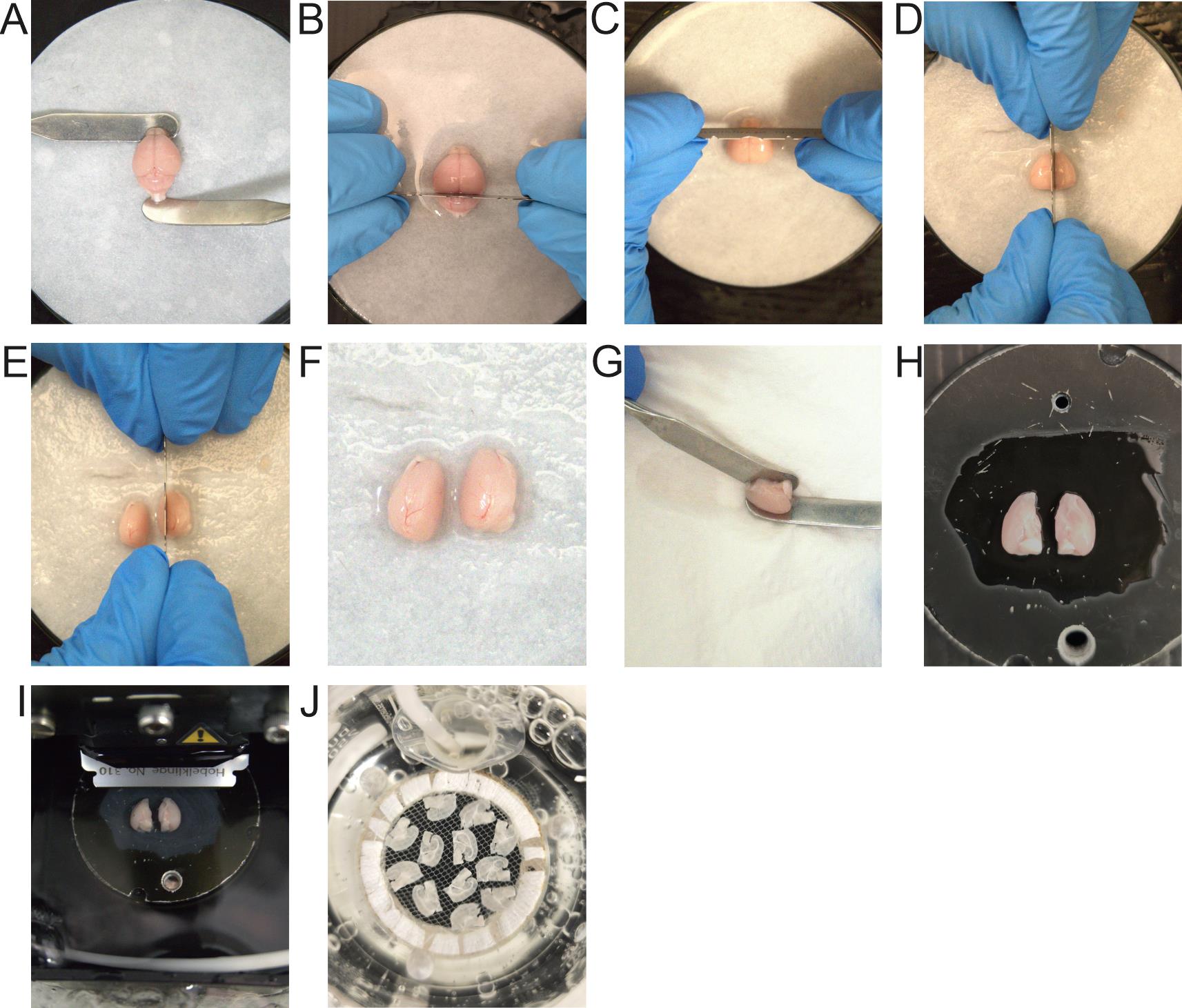
Figure 4. Dissection of cortico-hippocampal region and slice preparation. (A) Isolated brain. (B–F) Steps of the cutting procedure to isolate the cortico-hippocampal region. (G–H) Removal of excess solution from the sample and attachment to the plate. (I) Sectioning of the tissue. (J) Recovery beaker containing cortico-hippocampal slices.
G. Slice mounting on the chip
1. Equilibrate the 3D-MEA chip with carbogenated recording solution (see Recipes; Krebs solution for cerebellum slices, modified ACSF solution for prefrontal slices, Krebs high-potassium and high-calcium solution for cortico-hippocampal slices) and test if the chip is properly working following the indications in General note 1.
Note: Remember to carbogenate the recording solution during the entire experiment and turn on the temperature control in the BrainWave6 software, setting it to 32–34 °C.
Critical: The physiological temperature of 37 °C could induce degradation of the brain slice, affecting the recording. As a good compromise, a temperature of 32–34 °C could be used instead.
2. Place the Pasteur pipette near the wall of the 3D HD-MEA and remove the bulk of the recording solution. Half of the 3D HD-MEA should be empty to allow correct placement of the sample holder frame (Figure 5A–C).
3. Place the sample holder frame using fine tweezers or, alternatively, using the sample holder handling tool.
Caution: Pay attention not to touch the pillars of the chip.
4. Add some recording solution to cover the sample holder frame.
Note: Do not completely fill the 3D HD-MEA with the recording solution, since the second part of the sample holder will need to be inserted later.
5. Take a slice from the recovery beaker and place it in the center of the chip using a modified Pasteur pipette with the tip removed. The slice must be transferred with the first drop released from the modified Pasteur pipette, avoiding excess in the 3D HD-MEA (Figure 5D).
Note: Excessive release of solution could provoke overflow during the following steps.
Critical: Gently add a small amount of solution using a P200 precision pipette to relocate and/or to unfold your slice. If this process does not work, remove the slice using a modified Pasteur pipette and then restart from step G4.
6. Using IC Capture software, take a picture of the brain slice, ensuring that the entire surface of the electrode array is visible (Figure 5E).
7. Mount the sample holder silicone net on the sample holder insert using fine tweezers or the sample holder handling tool to insert the net ribs into the sample holder insert’s recesses.
8. Place the sample holder insert to stabilize the slice on the chip during the entire experiment. The sample holder insert must be positioned over the 3D HD-MEA using fine tweezers or the sample holder handling tool, after which it will slide down on its own (Figure 5F, G).
Caution: Avoid pressing the sample holder insert on the chip, since it could damage both the slice and the pillars of the chip.
Critical: Before placing the sample holder insert on the chip, ensure no air bubbles are trapped beneath the net holes (see Troubleshooting section, Problem 6).
Critical: Carry out steps G5–8 as quickly as possible to preserve slice viability, while taking care not to touch the center of the chip during the procedure.
9. Position the perfusion inlet above the chip center to allow the recording solution to drop directly onto the slice (Figure 5H).
Note: Direct dropping over the slice enables its adhesion to the chip surface.
10. Position the perfusion outlet out of the recording area, close to the reservoir wall, to continuously remove excess solution from the 3D HD-MEA.
Critical: The inlet and outlet flow rates and positions must be perfectly balanced to prevent spillage or drying of the 3D HD-MEA, which can alter the pressure applied by the sample holder insert, causing tissue-chip coupling issues.
11. Once the 3D HD-MEA is filled, the outlet removes the excess solution, maintaining a constant level and ensuring continuous renewal of the solution in the 3D HD-MEA.
12. The slice is now ready for recording.
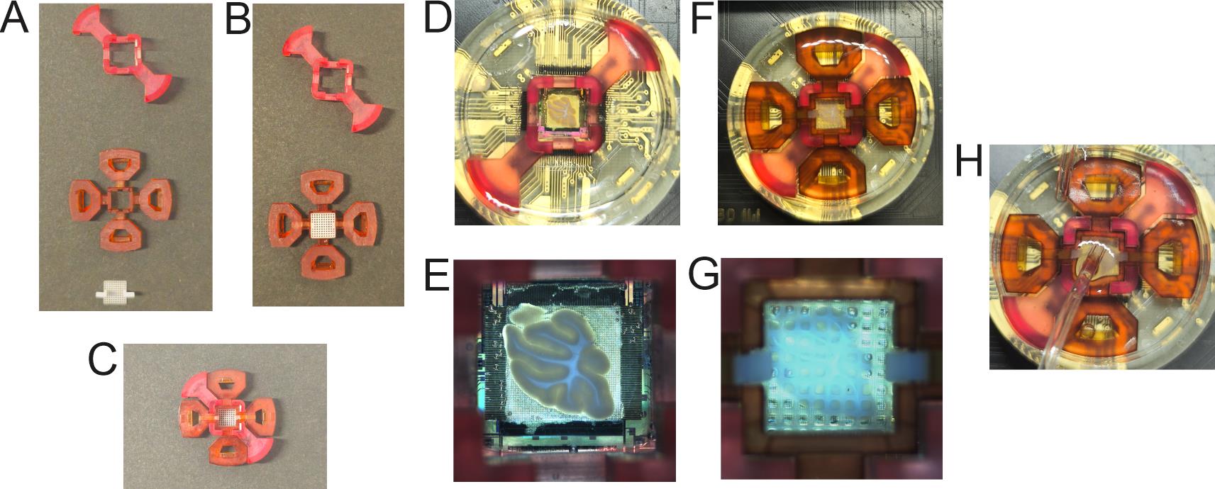
Figure 5. Preparation of the sample holder and mounting on the chip. (A) Components of the sample holder: frame (top), insert (middle), and the small white silicone net (bottom). (B) The silicone net is placed in the insert using fine tweezers. (C) The assembled sample holder. (D, E) Positioning of the frame and the slice over the chip. (F, G) Positioning of the insert. (H) Positioning of the perfusion inlet and outlet above the chip.
H. Recording of brain slices with 3D HD-MEA chip
1. Open BrainWave6 software and select Live Experiment.
2. In the control center of the recording view, set the Model to Brain Slice.
3. Set the Destination (file path) and Duration (recording time), then start the acquisition by clicking on the “play” button.
Note: Recording length should be customized to the user’s needs.
4. Go to the Overlay and Annotations tab of the software, open the Well Layers menu, and click the + button to add the slice image taken with the IC Capture software. Superimpose the image and set the opacity to 15%–20% to visualize both the activity map and the brain slice simultaneously.
Critical: Ensure that all four corners of the electrode array are clearly visible in the image and use the Align Selected Image Layer tool to obtain a precise overlay.
5. In the Chip Pilot tab, set the Hardware High-Pass filter cutoff frequency to 100 Hz for cerebellar slices or 10 Hz for prefrontal and cortico-hippocampal slices, to record both field potentials and spikes (Video 1).
Note: The hardware high-pass filter setting is crucial for recording both field potentials and spikes (Figure 6), as they have different temporal characteristics. In the cerebellar cortex, spontaneous slow field potential waves are not expected; therefore, a cutoff frequency of 100 Hz is recommended to stabilize the baseline. For prefrontal and cortico-hippocampal slices, a cutoff frequency between 5 and 20 Hz is recommended. The choice of the hardware high-pass filter cutoff frequency depends on the spectral content of the physiological signals of interest. Slow components, such as local field potentials, require a low cutoff frequency to avoid signal attenuation, whereas fast events, such as action potentials, benefit from a higher cutoff frequency. However, decreasing the cutoff frequency increases baseline fluctuations due to slow drifts and DC offsets. Therefore, the cutoff frequency must be selected as a compromise between preserving low-frequency signal components and maintaining baseline stability.
6. Click the “rec” button to start the recording.
Note: Before starting the recording, follow the instructions described in General note 4 to ensure stable acquisition.
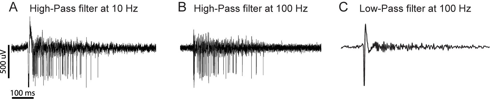
Figure 6. Effect of high-pass and low-pass filtering on prefrontal cortex signals. (A) High-pass filter at 10 Hz, showing both slow field potentials and fast spikes. (B) High-pass filter at 100 Hz, emphasizing fast spikes while attenuating slow components. (C) Low-pass filter at 100 Hz, isolating the low-frequency component (field potential).

I. Removing the sample from the 3D HD-MEA chip
1. Stop the perfusion system and remove the inlet and the outlet tubes.
2. Follow the instructions described in General note 2.
Data analysis
Brain slices data analysis
1. Use the Activity Groups tool to define regions of interest that follow the morphology of the slice. This ensures that all results are extracted according to specific slice regions (for image overlay, see step H4) (Figure 7).
2. Perform Spike Detection analysis to identify all action potentials by applying a High-Pass Filter with a cutoff frequency of 100 Hz to isolate the spiking component.
• For cortico-hippocampal and prefrontal slices, use the PTSD algorithm with the Standard Deviation Factor set to 8 and spike assignment set to Negative.
• For cerebellar slices, use a Hard Threshold algorithm with the threshold set to -100 μV. Leave all other parameters at their default values.
Note: Applying high-pass filter during the analysis helps the algorithm identify the correct signal by isolating spiking activity from slow field potentials. This is particularly important for prefrontal and cortico-hippocampal slice recordings acquired with a 10 Hz hardware high-pass filter.
Critical: The choice of spike detection algorithm depends on the activity level of the sample. Since the PTSD algorithm is based on noise standard deviation, samples exhibiting high tonic activity (as in cerebellar slices) may result in missed spikes or discarded active channels. In such cases, the hard-threshold algorithm is more appropriate.
3. Run a Spike Sorting analysis to associate clusters of action potentials detected by a single electrode with one or more neurons. Use PCA as the feature extraction method and K-Means with Gap Statistics as the clustering algorithm. Set the Maximum Number of Clusters to 3. To estimate the Minimum Number of Spikes per Cluster, use the standard firing rate definition:
where MFR is the mean firing rate, and T is the recording duration.
Additional steps for cerebellar slices (Figure 8A):
4. Analyze evoked and spontaneous activity using NeuroPULSE [31], following the instructions provided in the software documentation.
Additional steps for prefrontal (Figure 8B) and cortico-hippocampal (Figure 8C) slices only:
5. Perform Spike Burst analysis using the LogISI algorithm and set the Minimum Number of Spikes to 5.
6. Perform Spike Network Burst analysis to identify neuronal network patterns. If the samples show clear bursting activity, use the Firing-Based algorithm. Set the Valid Unit Threshold to 0.1 Hz (a canonical threshold to identify active channels, which can be adjusted based on the channel spiking activity) and the Bin Size to 50 ms (this value can be adjusted based on the duration of the network event), then click the “run” button to start the detection. Visualize the results using a raster plot. Increase the High Threshold Factor to reduce false positives or decrease it to detect missed bursts. Adjust the Low Threshold Factor to include or exclude additional events within a network burst.
Note: The Valid Unit Threshold should be adapted based on the level of activity in terms of frequency. The higher the activity of the recorded neuron, the higher this parameter can be set (e.g., cerebellar Purkinje neurons exhibit a basal activity >10 Hz).
Critical: If the samples contain multiple units with tonic firing activity, use the recruitment-based algorithm instead. Set the Valid Unit Threshold to 0.1, the Bin Size to 50 ms, and run the detection. Use the raster plot to evaluate and adjust the Recruited Valid Unit Threshold and Recruited Spike Threshold. Increasing these thresholds enables detection of smaller network bursts, whereas decreasing them restricts detection to larger bursts only.
7. Perform Field Potential Detection analysis by applying a Low-Pass Filter with a cutoff frequency of 100 Hz to isolate field potentials. Use both negative and positive thresholds (-100 and +100, respectively, to avoid noise detection) and adjust the Energy Window according to the expected field potential duration. Leave all other parameters at their default values.
Critical: The Energy Window parameter is used to extend the detection window, since field potentials are slow-wave events. As a result, they may cross the detection threshold several milliseconds after the actual onset of the event and may fall below the threshold before the event has fully ended.
8. If multiple field potentials occur consecutively (e.g., epileptic activity), perform a Field Potential Burst Detection using default parameters.
9. Perform Field Potential Network Burst analysis to identify activity patterns. If clear network bursting is present, use the Firing-Based algorithm. Set the Valid Unit Threshold to 0.1 fp/min and the Bin Size to 2 s, then click the “run” button to start the detection. Use a raster plot to visualize the results and adjust threshold factors as needed.
10. Before plotting the analysis results, create an additional grouping of electrodes to separate active from inactive units. This grouping can be based on one or more analysis-derived metrics (e.g., Mean Firing Rate > 0.1 spk/s). Ensure that only units located within the slice boundaries are included and exclude all units outside the slice.
11. Plot the desired charts by selecting Visible Activity Groups in the Regions To Plot settings and export the corresponding data using the export tool.
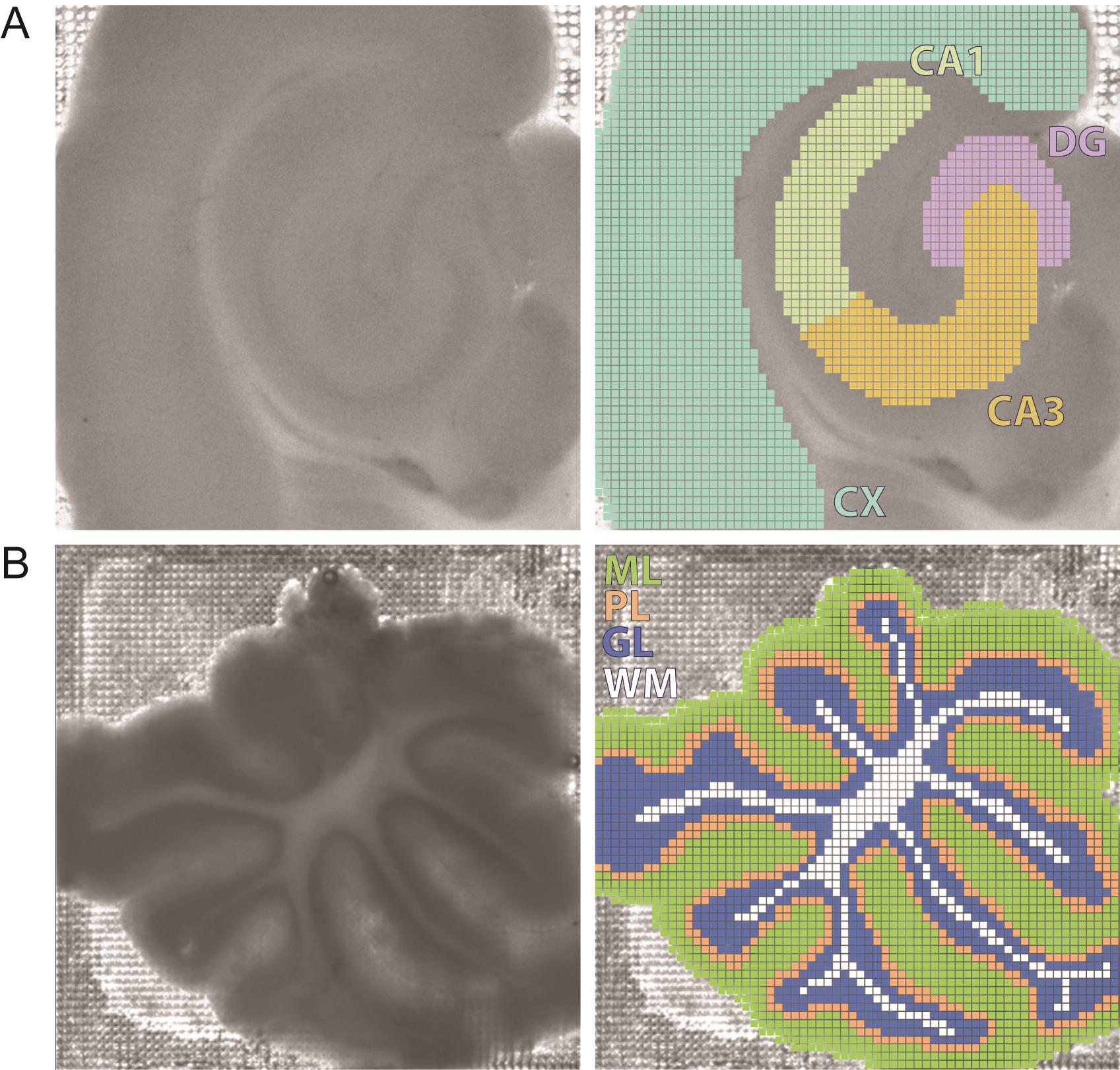
Figure 7. Overlay of the slice image on the 3D HD-MEA chip and channel selection for precise anatomical identification. (A) Cortico-hippocampal slice. (B) Cerebellar slice. Abbreviations: DG, dentate gyrus; CA3, cornu ammonis area 3; CA1, cornu ammonis area 1; CX, cortex; ML, molecular layer; PL, Purkinje cell layer; GL, granular layer; WM, white matter.
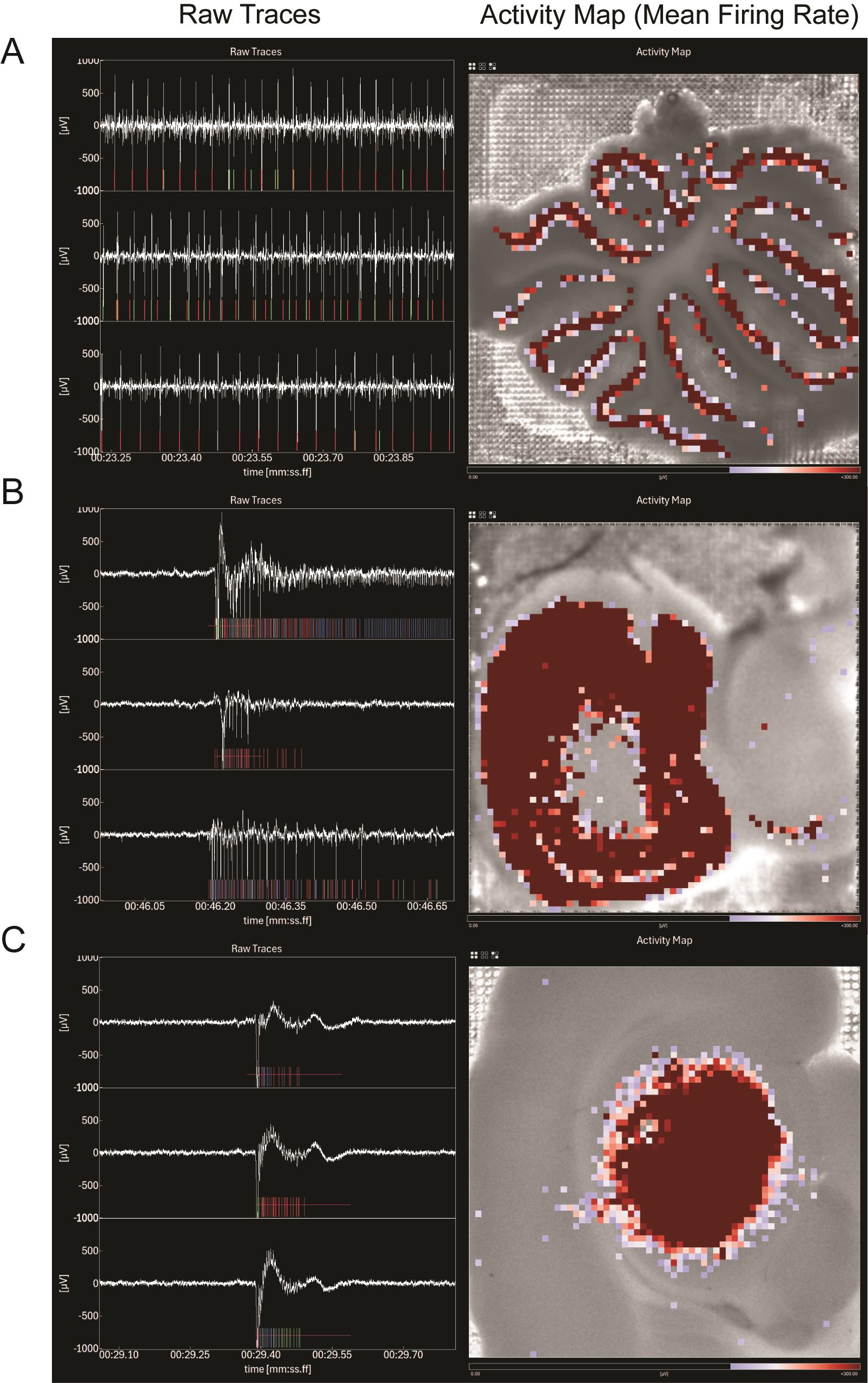
Figure 8. Typical recorded activity maps (on the right) and corresponding raw traces (on the left) of acute slices collected from different brain regions. (A) Cerebellar, (B) cortico-hippocampal, and (C) prefrontal slices. Detected spikes are marked with vertical lines (each color corresponds to a specific unit defined by spike sorting), and detected field potential and spike bursts are indicated by separated horizontal lines.
Part II: Brain spheroids and region-specific neural organoids
Materials and reagents
Biological materials
Brain spheroids
1. Rat cortex or hippocampal primary neurons (obtained from rat dissection in-house)
2. NPC-derived neurons (generated in-house from commercial human iPSC lines)
Neural organoids
1. Human iPSC cell line C4.1 was used for spinal cord organoids (female; origin: previously generated from cord blood of an unidentified healthy control individual; non-commercially available). Cells were maintained on vitronectin-coated plates (Thermo Fisher Scientific, catalog number: A14700) in Essential 8 medium (Thermo Fisher Scientific, catalog number: A1517001). Genomic integrity was confirmed by single-nucleotide polymorphism array analysis, and cultures were routinely screened for Mycoplasma contamination [32–34].
2. Human iPSC cell line TFSi001-A (Thermo Fisher Scientific) was used for cortical organoids. Cultures were cultured on hLaminin-521-coated Petri dishes in StemFlexTM medium (Thermo Fisher Scientific, catalog number: A3349401). Cultures were routinely screened and confirmed negative for Mycoplasma contamination.
Reagents
Brain spheroids
1. Neurobasal Plus medium (Thermo Fisher Scientific, Gibco, catalog number: A358290)
2. B-27TM Plus neuronal culture system (Thermo Fisher Scientific, Gibco, catalog number: A3653401)
3. RevitaCellTM supplement (100×) (Thermo Fisher Scientific, Gibco, catalog number: A2644501)
4. Neurobasal medium (Thermo Fisher Scientific, Gibco, catalog number: A1647801)
5. Advanced DMEM/F-12 (Thermo Fisher Scientific, Gibco, catalog number: 12634010)
6. Neural induction supplement (Thermo Fisher Scientific, Gibco, catalog number: A1647801)
7. Neurobasal medium (Thermo Fisher Scientific, Gibco, catalog number: 21103049)
8. CultureCEPTTM supplement (1,000×) (Thermo Fisher Scientific, Gibco, catalog number: A56799)
9. GlutaMAXTM supplement (Thermo Fisher Scientific, Gibco, catalog number: 35050061)
10. N-2 supplement (100×) (Thermo Fisher Scientific, Gibco, catalog number: 17502048)
11. CultureOneTM supplement (100×) (Thermo Fisher Scientific, Gibco, catalog number: A3320201)
12. L-ascorbic acid (Merck, Sigma-Aldrich, catalog number: A92902)
13. Human GDNF recombinant protein (Thermo Fisher Scientific, PeproTech, catalog number: 450-10-50UG)
14. Human/Mouse/Rat BDNF recombinant protein (Thermo Fisher Scientific, PeproTech, catalog number: 450-02-10UG)
15. rhLaminin-521 (Thermo Fisher Scientific, Gibco, catalog number: A29249)
16. DPBS, no calcium, no magnesium (Thermo Fisher Scientific, Gibco, catalog number: 14190144)
Neural organoids
1. Neurobasal A (United States Biological, catalog number: N1020-02)
2. B-27 supplement without vitamin A (Life Technologies, catalog number: 12587010)
3. Penicillin-Streptomycin (Cytiva, catalog number: SV30010)
4. Glutamax (Thermo Scientific, catalog number: 35050061)
5. N2 supplement (Life Technologies, catalog number: 17502048)
6. Human recombinant BDNF (PeproTech, catalog number: 450-02)
7. Human recombinant IGF-I (PeproTech, catalog number: 100-11)
8. L-ascorbic acid (Sigma-Aldrich, catalog number: A4403)
9. Cyclic adenosine monophosphate (cAMP) (Sigma-Aldrich, catalog number: D0627)
10. Anti-adherence rinsing solution (STEMCELL Technologies, catalog number: 07010)
11. Essential 6TM Medium (Thermo Fisher Scientific, catalog number: A1516401)
12. Dorsomorphin dihydrochloride (R&D systems, catalog number: 3093)
13. SB 431542 (Selleckchem, catalog number: S1067)
14. Y-27632/Rock inhibitor (R&D systems, catalog number: 1254)
Solutions
Brain spheroids
1. Neurobasal Plus complete medium (see Recipes)
2. Neural expansion medium (see Recipes)
3. Neural differentiation medium (see Recipes)
Neural organoids
4. Neurobasal base medium (see Recipes)
5. Spinal cord organoid (hSpO) medium (see Recipes)
Recipes
Brain spheroids
1. Neurobasal Plus complete medium
| Reagent | Final concentration | Quantity or volume |
|---|---|---|
| NeuroBasal Plus | n/a | 48.5 mL |
| B27 Plus supplement 50× | 1× | 1 mL |
| Glutamax | 1× | 500 μL |
| Gentamicin | 0.015 mg/mL | 75 μL |
| RevitaCell (optional) | 1× | 500 μL |
| Total | n/a | 50 mL |
2. Neural expansion medium
| Reagent | Final concentration | Quantity or volume |
|---|---|---|
| Neurobasal medium | n/a | 24 mL |
| Advanced DMEM/F-12 | n/a | 24 mL |
| Neural induction supplement | 1× | 1 mL |
| Glutamax | 1× | 500 μL |
| Gentamicin | 0.015 mg/mL | 75 μL |
| CultureCEPTTM (optional) | 1× | 50 μL |
| Total | n/a | 50 mL |
3. Neural differentiation medium
| Reagent | Final concentration | Quantity or volume |
|---|---|---|
| NeuroBasal Plus | n/a | 48.5 mL |
| B27 Plus supplement 50× | 1× | 1 mL |
| N-2 supplement | 1× | 500 μL |
| CultureOne supplement | 1× | 1 mL |
| L-ascorbic acid | 200 μM | n/a |
| Human GDNF | 10 ng/mL | n/a |
| Human BDNF | 20 ng/mL | n/a |
| Glutamax | 1× | 500 μL |
| Gentamicin | 0.015 mg/mL | 75 μL |
| Total | n/a | 50 mL |
Neural organoids
4. Neurobasal base medium
| Reagent | Final concentration | Quantity or volume |
|---|---|---|
| Neurobasal medium | n/a | 960 mL |
| B-27 without vitamin A | 50× | 20 mL |
| Pen/Strep | 100× | 10 mL |
| Glutamax | 100× | 10 mL |
| Total | n/a | 1,000 mL |
5. Spinal cord organoid media
| Reagent | Final concentration | Quantity or volume |
|---|---|---|
| Neurobasal base medium | n/a | 50 mL |
| N-2 supplement | 100× | 500 μL |
| BDNF | 20 ng/mL | 50 μL |
| IGF-1 | 10 ng/mL | 50 μL |
| L-ascorbic acid | 200 μM | 50 μL |
| cAMP | 50 μM | 25 μL |
Laboratory supplies
Brain spheroids
1. Filter tip, 10 μL (Sarstedt, catalog number: 70.3010.255)
2. Filter tip, 20 μL (Sarstedt, catalog number: 70.3030.265)
3. Filter tip, 200 μL (Sarstedt, catalog number: 70.3031.255)
4. Filter tip, 1,000 μL (Sarstedt, catalog number: 70.1186.210)
5. 96-well ultra-low attachment plate (Sarstedt, catalog number: 83.3925.400)
6. Serological pipette, with tip, plugged, 25 mL (Sarstedt, catalog number: 86.1685.001)
7. Serological pipette, with tip, plugged, 10 mL (Sarstedt, catalog number: 86.1254.001)
8. Serological pipette, with tip, plugged, 5 mL (Sarstedt, catalog number: 86.1253.001)
9. SafeSeal reaction tube, 5 mL (Sarstedt, catalog number: 72.701.400)
10. SafeSeal reaction tube, 1.5 mL (Sarstedt, catalog number: 72.706.400)
11. Tissue culture dish, 100 × 20 mm (Sarstedt, catalog number: 83.3902)
12. Suction filtration flask (Fisher Scientific, catalog number: 15844498)
Neural organoids
1. Filter tip, 200 μL (VWR, catalog number: 76322-150)
2. Filter tip, 20 μL (VWR, catalog number: 76322-134
3. Filter tip, 1000 μL (VWR, catalog number: 76322-154)
4. Conical tube, 50 mL (VWR, catalog number: 21008-736)
5. Conical tube, 15 mL (VWR, catalog number: 21008-671)
Equipment
Brain spheroids and neural organoids
1. FinnpipetteTM F2 0.2–2 μL, 2–20 μL, 20–200 μL, 100–1,000 μL (Thermo Scientific, catalog numbers: 4642010, 4642060, 10413865, 11877351)
2. FinntipTM wide orifice pipette tips (Thermo Scientific, catalog number: 9405020)
3. Digital microscope (Dino-Lite Digital Microscope, model: AM73515MZTL)
4. Digital microscope stand (Dino-Lite Digital Microscope, model: RK-06A)
5. BioCAM (3Brain, model: DupleX)
6. 3D HD-MEA (3Brain, model: CorePlateTM 3D 1W 38-60-90)
7. Mini-incubator box (3Brain)
8. 5%–10% carbon dioxide/air tank (Air Liquide)
9. Sample holder frame (3Brain, model: Sample Holder 2, Frame)
10. Sample holder insert (3Brain, model: Sample Holder 2, 500, 750, 1000, 1,250 μN)
11. Sample holder silicone net (3Brain, model: Sample Holder 2, Silicone Net)
12. Sample holder handling tool (3Brain, model: Sample Holder 2, Handling tool)
13. Steri-Cult CO2 incubator (Thermo Fisher, model: 3307)
14. MSC-AdvantageTM Class II Biological Safety Cabinet (Thermo Fisher, catalog number: 51025413)
15. SL 8 small benchtop centrifuge (Thermo Fisher, catalog number: 75007221)
16. Tacta® mechanical pipettes (Sartorius, catalog number: LH-729673)
17. PrecisionTM general purpose baths (Thermo Fisher, catalog number: TSGP10)
18. S1 pipette fillers (Thermo Fisher, catalog number: 9531)
19. Inverted microscope (Olympus, catalog number: CKX53)
20. Microscope camera (Olympus, catalog number: EP50)
Software and datasets
1. Software 1 BrainWave6 (3Brain), requires a license
2. Software 2 Dino Capture (Dino-Lite Digital Microscope, Version 2.0)
Procedure
A. Generation of primary rat neuronal spheroids
1. Isolate (or thaw) rat cortex or hippocampal primary neurons from dissection [35].
2. Prepare single-cell suspensions using NeuroBasal Plus complete medium (if the cells are thawed, supplement them with RevitaCell or a similar supplement designed to improve survival after thawing).
3. Perform cell counting using a Burker chamber or an automated cell counter.
4. Dilute the cells to obtain final concentrations of 500 and 1,000 cells/μL in NeuroBasal Plus complete medium.
5. To generate spheroids with diameters of approximately 400–500 μm or 700–800 μm at ~3 weeks after plating, dispense 50 μL per well containing approximately 25,000 cells or 50,000 cells, respectively, into each well of a 96-well ultra-low attachment plate.
6. After 24 h, spheroids should have already formed. Gently add an additional 150 μL of medium to each well to dilute the RevitaCell supplement.
7. Subsequently, replace approximately 50% of the medium every 3–4 days to maintain spheroid growth and viability (Figure 9A).
B. Generation of hiPSC-NPC-derived neuronal spheroids
1. Neural progenitor cells (NPCs), generated using the desired protocol, were cultured in neural expansion medium (NEM) on 100 mm tissue culture-treated dishes coated with 3.33 μg/mL recombinant human laminin-521 (rhLaminin-521; 1:30 dilution from a 100 μg/mL stock) until they reached ~70% confluency [36].
2. Remove the spent medium from the 100 mm dish and wash once with 8 mL of DPBS without CaCl2 and MgCl2.
3. After removing DPBS, detach NPCs by adding 5 mL of prewarmed StemPro Accutase cell dissociation reagent to the 100-mm dish. Incubate at 37 °C for 5–7 min, until cells are visibly rounded and begin detaching from the surface.
4. Collect the cells by adding 10 mL of neural expansion medium (NEM) supplemented with CultureCEPT (or a similar ROCK inhibitor).
5. Centrifuge the cell suspension at 200× g for 5 min.
6. Resuspend the pellet in NEM [36] supplemented with CultureCEPT (or similar ROCK inhibitors) to obtain a single-cell suspension.
7. Perform cell counting using a Burker chamber or an automated cell counter.
8. Dilute the cells to obtain final concentrations of 300 cells/μL and 700 cells/μL in neural expansion medium supplemented with CultureCEPT.
9. To generate spheroids with diameters of approximately 400–600 or 1,000–1,200 μm, at ~4 weeks after plating, dispense 50 μL per well containing approximately 15,000 or 35,000 cells, respectively, into each well of a 96-well low-attachment plate.
Note: Final spheroid size may vary depending on the proliferation rate of the specific cell line used.
10. After 24 h, spheroids should have already formed. Gently add an additional 150 μL of medium to each well.
11. Subsequently, replace approximately 50% of the medium every other day to maintain spheroid growth and viability (Figure 9).
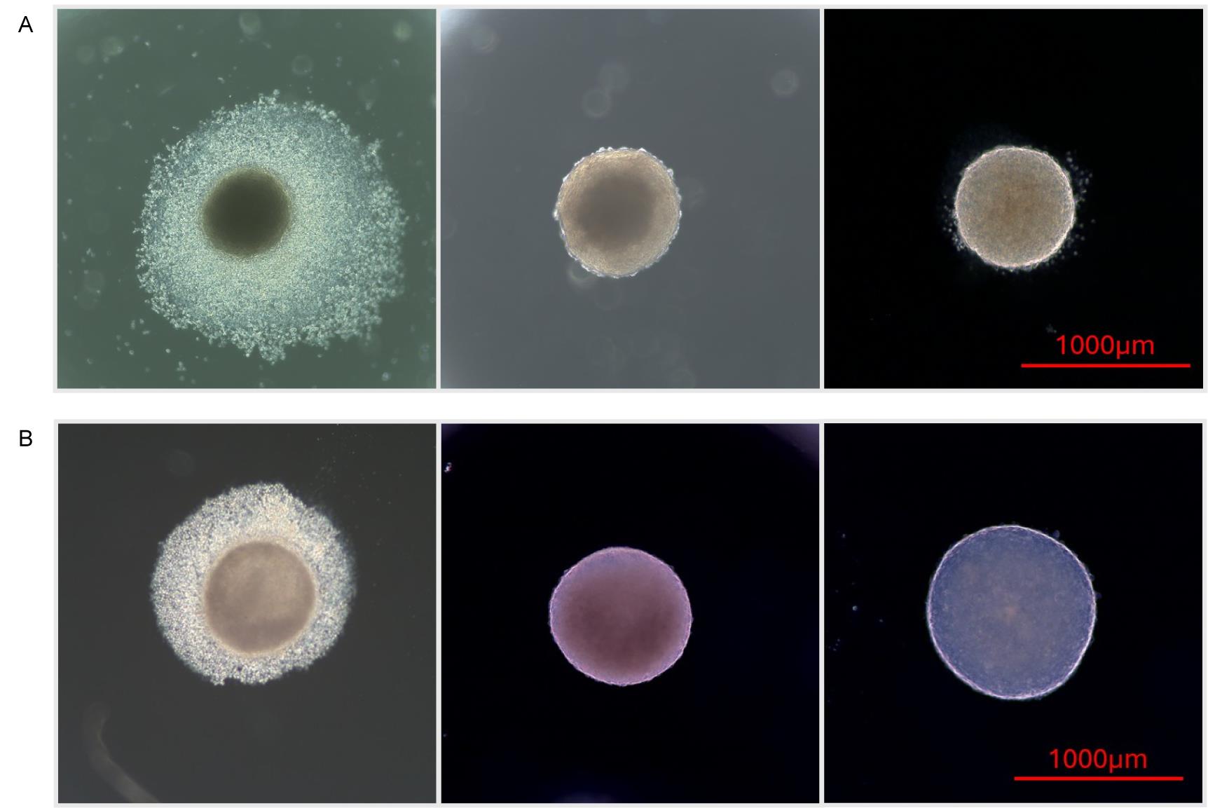
Figure 9. Development and progression of spheroid formation from rat cortical neurons (A) and human induced pluripotent stem cell (iPSC)-derived neurons (B). Day 1 (left): Initiation of spontaneous cell aggregation observed 24 h post-seeding. Around the forming spheroid, cells in the early stages of aggregation are also observed. Dead cells are subsequently eliminated through repeated medium changes. Day 7 (middle): Fully formed spheroids after 7 days of culture. Day 14 (right): Mature spheroid exhibiting spherical shape and advanced structural organization. Scale bars: 1,000 μm.
C. Generation of hiPSC-derived cortical organoids and spinal cord organoids
1. Maintain hiPSCs in Essential 8 medium (or medium of choice) on vitronectin-coated (or alternative coating) plates and expand to ~80%–90% confluency in 100 mm dishes.
2. Wash once with PBS without Ca2+/Mg2+ and dissociate cells using Accutase (7–10 min at 37 °C) until ≥90% detachment; gently triturate to obtain a single-cell suspension.
3. Dilute the Accutase 1:1 with Essential 8 medium supplemented with 10 μM Y-27632 (ROCK inhibitor), centrifuge at 200× g for 5 min, resuspend the cell pellet, and perform cell counting.
4. Pretreat AggreWellTM 800 plates according to the manufacturer’s instructions. After pretreatment, add 1 mL of Essential 8 medium supplemented with ROCK inhibitor to each well and equilibrate in the incubator.
5. Prepare a single-cell suspension at ~3 × 10⁶ cells/mL in Essential 8 medium with ROCK inhibitor, then add 1 mL of the cell suspension per AggreWell well (final volume of 2 mL; ~3 × 10⁶ cells per well).
6. Centrifuge AggreWell plates at 200× g for 5 min and incubate for 24 h to generate uniform embryoid bodies.
7. After 24 h (on day 0), transfer embryoid bodies to ultra-low attachment plates in Essential 6 medium supplemented with Dorsomorphin (2.5 μM), SB-431542 (10 μM), and ROCK inhibitor (10 μM).
8. After day 0, patterning molecules are used to guide regional fate.
C1. To generate cortical organoids following existing protocols [15,37]:
9. From day 1 to day 5, maintain organoids in Essential 6 medium supplemented with Dorsomorphin (2.5 μM) and SB-431542 (10 μM). Change media daily.
10. From day 6 to day 25, transition organoids to Neurobasal-A-based medium supplemented with FGF2 (20 ng/mL) and EGF (20 ng/mL). Change media every 1–2 days.
11. From day 26 to day 44, maintain organoids in Neurobasal-A-based medium supplemented with BDNF (20 ng/mL) and NT-3 (20 ng/mL). Change media every 2–3 days.
12. From day 45 onward, maintain organoids in Neurobasal-A-based medium without additional patterning factors, following routine feeding schedules every 3–4 days.
C2. To generate spinal cord organoids following existing protocols [11,38]:
13. From day 1 to day 2, maintain organoids in Essential 6 medium supplemented with Dorsomorphin (2.5 μM) and SB-431542 (10 μM).
14. From day 3 to day 4, maintain organoids in Essential 6 medium supplemented with Dorsomorphin (2.5 μM), SB-431542 (10 μM), and CHIR99021 (3 μM).
15. From day 5 to day 8, transition organoids to Neurobasal-A-based medium supplemented with EGF (20 ng/mL), FGF2 (10 ng/mL), retinoic acid (0.1 μM), and CHIR99021 (3 μM). Change media daily.
16. From day 9 to day 16, maintain organoids in Neurobasal-A-based medium supplemented with EGF (20 ng/mL), FGF2 (10 ng/mL), retinoic acid (0.1 μM), CHIR99021 (3 μM), and SAG (100 nM). Change media every 2 days.
17. From day 17 to day 22, maintain organoids in Neurobasal-A-based medium supplemented with N-2, BDNF (20 ng/mL), cAMP (50 μM), ascorbic acid (200 μM), IGF (10 ng/mL), and DAPT (2.5 μM). Change media every 2 days.
18. From day 23 onward, maintain organoids in Neurobasal-A-based medium supplemented with N-2, BDNF (20 ng/mL), cAMP (50 μM), ascorbic acid (200 μM), and IGF (10 ng/mL). Change media every 2–3 days.
Notes:
1. Detailed protocols and demonstration videos on hiPSC thawing, maintenance, passaging, and organoid differentiation are available at www.brainorganoidhub.com/protocols.
2. Throughout the organoid culture, the samples are maintained in a 100 mm cell culture dish pretreated for 2 min with 6 mL of anti-adherence rinsing solution.
D. Transition brain spheroids/neural organoids from incubation to measurement
1. Prewarm the recording media at 37 °C.
2. Move the low adhesion plate from the incubator to the laminar hood, ensuring the sterility of the samples.
3. To harvest a spheroid, gently flush the media inside a well by using a P200 pipette with the tip cut to detach the samples from the bottom of the well. Use a dark background to visualize the samples (Figure 10A).
Notes:
1. Step D3 is not necessary for organoids.
2. Spheroids are cultured on a low-adhesion plate in the incubator, and organoids are kept on a 100 mm Petri dish previously treated with anti-adherence rinsing solution. Since acute measurements are performed in a non-sterile environment, only the samples selected for electrophysiological experiments should be harvested.
4. Carefully aspirate all the media and the sample with a pipette. Transfer the spheroids into a Petri dish (35 or 100 mm, depending on the number of samples to be collected). Aspirate the organoids with a P1000 pipette with the tip cut and transfer them into 1.7 mL tubes instead (Figure 10B). Repeat this step for all the samples that must be used during the experimental session. Add enough medium to the Petri dish or tube to ensure that the samples remain fully submerged and to prevent complete evaporation.
Note: The recording area of the 3D HD-MEA of 3.8 by 3.8 mm2 can accommodate multiple samples, facilitating simultaneous data collection and increasing the efficiency of the experimental session.
5. Keep the Petri dish or tubes with the samples in the incubator during intervals between measurements.
E. 3D HD-MEA setup preparation
1. Prepare the setup as shown in Figure 10B:
a. Connect a 5%–10% carbon dioxide/air tank to a suction filtration flask filled with sterile double deionized water (DDW) and then to the mini-incubator box (Figure 10B).
b. Place the digital microscope on top of the recording area of a 3D HD-MEA locked inside the BioCAM (Figure 10B).
2. Choose the holder according to the spheroid size:
a. For brain spheroids of ~400/500 μm, use a 1,250 μN holder to ensure stable contact without mechanical stress.
b. For brain spheroids of ~1,000/1,200 μm, use lighter holders (750 or 1,000 μN).
c. For neural organoids of ~1,000/1,700 μm, use a 750 μN holder.
d. For neural organoids >1,700 μm, use lighter holders (500 μN).
Note: The proposed holder type could be subjected to modification based on the number of samples loaded, size, age, and cellular composition of the neural organoid or brain spheroid.
3. Mount the sample holder silicone net on the sample holder insert using fine tweezers or the handling tool to place the net ribs into the sample holder insert's recesses (Figure 10B).
4. Place the sample holder insert into a 35 mm Petri dish filled with culture media or PBS to hydrophilize the sample holder silicone net. Then, flush the solution through the net by using a P1000 pipette to remove any air bubbles trapped in the net holes.
5. Mount the sample holder’s frame inside the 3D HD-MEA well using fine tweezers or the handling tool (Figure 10C).
6. Equilibrate the 3D HD-MEA with some media solution and test that the chip is properly working, following the instructions in General note 1.
7. Fill the 3D HD-MEA well with 2.5 mL of warm culture media to completely cover the sample holder frame.
8. Start Dino Capture software and set the focus and image dimension of the digital microscope to visualize the grid of the electrodes of the 3D HD-MEA.
9. Turn on the temperature control in BrainWave6 and set it at 37 °C.
F. Sample mounting procedure
1. Depending on your experimental needs, take one or more spheroids/organoids from the Petri dish or the 1.7 mL tube by using a P200 or P1000 pipette with the tip cut. Aspirate as little media as possible. In case of brain spheroids collected in the Petri dish, use a dark background to visualize the samples (Figure 10A).
2. Move the pipette containing the spheroids/organoids on top of the electrode array and gently flush to release the samples onto the recording area.
Critical: Avoid touching the electrodes with the pipette tip, as they may bend or break, compromising proper functioning.
3. Allow the spheroids/organoids to sink and settle on the electrode array. Gently flush the media around the recording area to center the samples if they landed on the edge of the electrode grid (Figure 10C). Once the samples are properly positioned, take a picture, ensuring that the entire electrode array is visible. Using a pair of fine tweezers, grab the sample holder insert from the hole of one of its wings. Remove excess media/PBS from the net with blotting paper. Alternatively, the sample holder insert can be easily grabbed and moved by using the holder handling tool.
Note: Keep the tweezers/holder handling tool perpendicular to the sample holder insert surface to facilitate proper positioning into the sample holder frame.
4. Carefully place the sample holder insert into the sample holder frame, aligning its wings with the sample holder frame openings. Gently move the sample holder insert toward the sample to break the liquid surface tension. Once the sample holder insert is completely submerged, release it; it will slowly sink onto the spheroids/organoids, holding them in place (Figure 10C).
Note: If the spheroids/organoids moved after the placement of the sample holder insert, take a new picture.
Caution: Avoid pressing the sample holder insert on the chip, since it could stress the spheroids/organoids and damage the pillars of the chip.
Critical: Before placing the sample holder insert on the chip, ensure no air bubbles are trapped in the net holes (see Troubleshooting, Problem 6).
5. Place the mini-incubator box on the 3D HD-MEA and open the 5%–10% carbon dioxide/air tank pressure regulator until you see steady bubbling in the filtration flask.
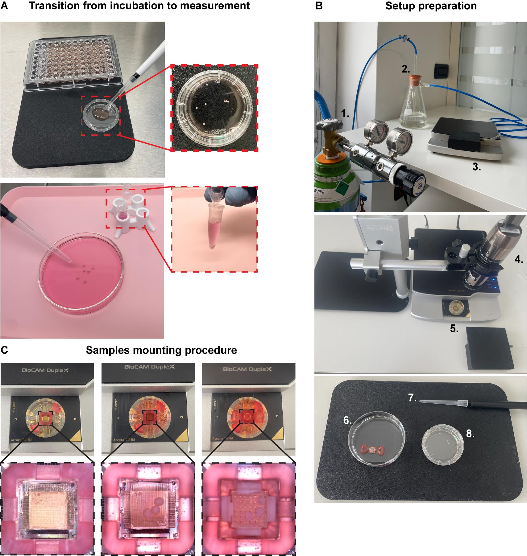
Figure 10. Setup and mounting procedure for brain spheroids/neural organoids. (A) Use a cut-tip P200 pipette to harvest brain spheroids from a 96-well low adhesion plate into a Petri dish; a dark background helps visualize samples (top). Organoids are transferred from a Petri dish to a 1.7 mL tube by using a P1000 with the tip cut; no dark background is needed (bottom). (B) System setup: 1, 5%–10% carbon dioxide/air tank; 2, suction filtration flask; 3, mini-incubator box; 4, digital microscope mounted on its stand; 5, 3D HD-MEA locked into the BioCAM; 6, sample holder silicone net attached to the sample holder insert; 7, P200 or P1000 pipette with the tip cut; 8, spheroids/organoids are taken out from the incubator only during the mounting procedure. (C) Insert the sample holder frame into the 3D HD-MEA well (left), fill the reservoir with 2.7 mL of culture media, then place the samples on the recording area (middle). Finally, gently lower the sample holder insert to secure the spheroids/organoids in place (right).
G. Recording of brain spheroids/neural organoids with 3D HD-MEA chip
1. Open BrainWave6 software and select Live Experiment.
2. In the control center of the recording view, set the Model to 3D cell culture, the Destination (file path), and Duration (recording time), then start the acquisition by clicking on the play button.
Note: Recording length should be customized to the user’s needs.
3. Go to the Overlay and Annotations tab of the software, open the Well Layers menu, and click the + button to add the spheroid/organoid image taken with the digital microscope. Superimpose the image and set the opacity to 15%–20% to visualize both the activity map and the organoid simultaneously.
4. In the Chip Pilot tab, set the Hardware High-Pass filter cutoff frequency to 100 Hz.
5. Click the “rec” button to start the recording (Videos 2 and 3).
Note: Before starting the recording, allow the samples to settle on the chip in the environmental control chamber for at least 5–10 min, depending on size and density.
H. Removing the samples from the 3D HD-MEA chip
1. Once the recording is complete, close the 5%–10% carbon dioxide/air tank pressure regulator and remove the mini-incubator box.
2. Follow the instructions described in General note 2.
Data analysis
A. Spheroid analysis (manual settings)
1. Use the Zone tool to define regions of interest that follow the morphology of each spheroid (Figure 11A). This ensures that results are extracted independently for each spheroid (for image overlay, see step E4).
Note: Each 3D HD-MEA can accommodate one or more spheroids simultaneously. Regardless of the number loaded, each sample should be considered an independent entity with no interaction with the others.
2. Run a Spike Detection analysis to locate all generated action potentials. Use the PTSD algorithm [39] with the Standard Deviation Factor set to “8” and spike assignment set to “negative”. Keep the other settings as default.
3. Run a Spike Sorting analysis to associate clusters of action potentials detected by a single electrode with one or more neurons (Figure 11). Use the PCA for feature extraction and the K-Means and Gap Statistics for clustering, setting the Maximum Number of Clusters at 3. Following the standard definition of firing rate, to estimate the Minimum Number of Spike per Cluster, use the formula:
where MFR is the mean firing rate, and T is the duration of the recording.
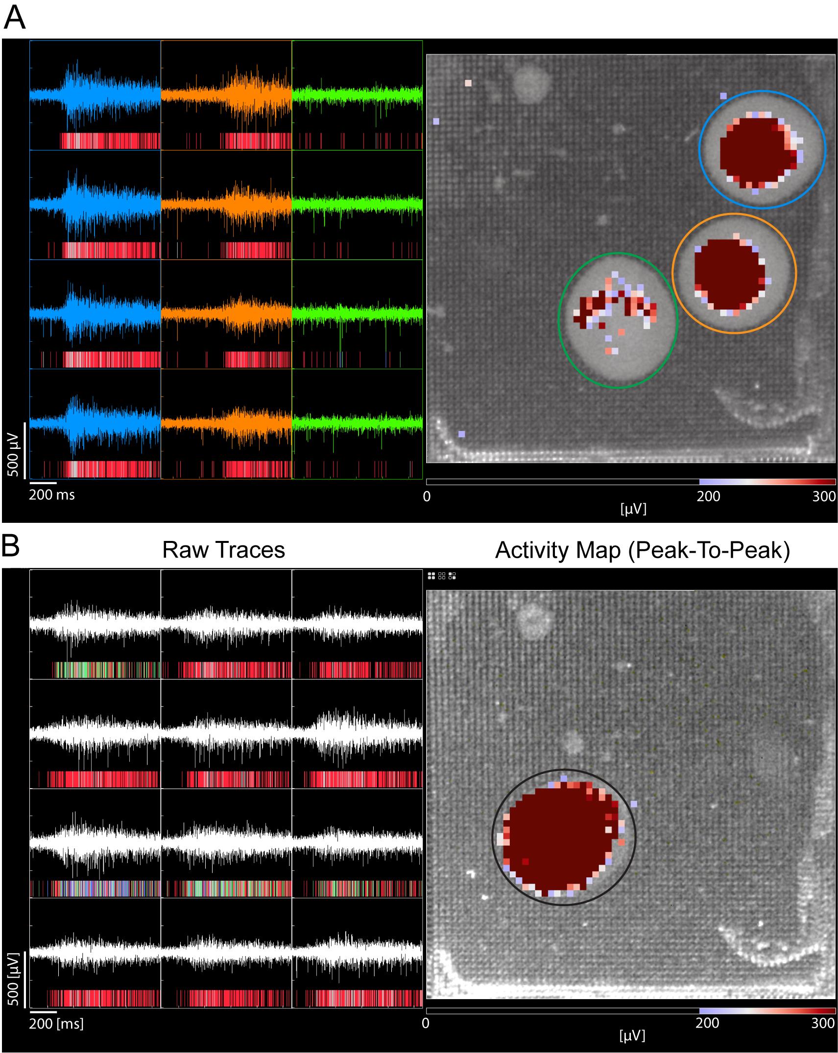
Figure 11. Raw traces and activity map of brain spheroids. (A) Voltage raw data traces (left) and peak-to-peak activity map (right) of three brain spheroids on a single 3D HD-MEA, each assigned to a color-coded zone. (B) Voltage raw data traces (left) and peak-to-peak activity map (right) from a single brain spheroid on a 3D HD-MEA. Colored bars under each trace mark detected action potentials, with each color representing a distinct neuron identified by spike sorting.
4. Run a Spike Burst analysis using the LogISI algorithm and set the Minimum Number of Spikes to 5.
5. Run a Spike Network Burst analysis to identify neuronal network patterns. If the samples exhibit clear bursting activity, use the Firing Based algorithm to accurately detect network bursts. To apply the appropriate settings, set the Valid Unit Threshold to 0.1 Hz and the Bin Size to 50 ms, then run the detection. A raster plot can be used to visualize the analysis results. Increase the High Threshold Factor to reduce false-positive network bursts or decrease it to capture bursts that may have been missed. Change the Low Threshold Factor to include or exclude additional events within a network burst. If the samples contain multiple units with tonic firing activity, use the Recruitment Based algorithm instead. Set the Valid Unit Threshold to 0.1, the Bin Size to 50 ms, and then run the detection. With the help of the raster plot, evaluate eventual changes in the analysis settings. Adjust both the Recruited Valid Unit Threshold and the Recruited Spike Threshold according to the number of units contributing to a network burst. Increasing these thresholds allows the detection of smaller network bursts, whereas decreasing them restricts detection to larger network bursts only.
6. Before plotting the results, perform additional grouping of the electrodes to separate the active units from the inactive ones.
Note: Grouping can be based on one or more metrics derived from previous analyses (e.g., Mean Firing Rate > 0.1 spk/s). Include only units located within the spheroid boundaries and remove any units outside.
7. Plot all the desired charts by selecting Visible Zones in the setting Regions To Plot and by selecting Visible Activity Groups in the setting Regions in subplots.
B. Organoid data analysis (experiment report)
1. Open BrainWave6 software and navigate to the Start Screen.
Note: The BrainWave6 software offers the option to automatically generate an experiment report based on a predefined set of selected settings. The following brain organoid analysis was performed using this automated reporting modality.
2. Select Generate Experiment Report to analyze a single recording or Batch Experiment Report to process multiple recordings simultaneously.
3. The first page to appear is the General Settings page. In the Source Selection panel, click Browse and select the raw MEA recording file(s) to be analyzed.
4. (Optional) In the Experiment Tags field, add descriptive tags to each recording (e.g., genotype, treatment condition, recording day).
Note: Experiment Tags function as metadata and can be used later for filtering and organization within BrainWave6.
5. Specify the Experiment Files Destination by selecting the folder where analysis outputs and reports will be saved.
6. Define the report file name using the File Name option. Select Same as Source to automatically assign the report the same name as the raw recording file, or alternatively, enter a custom file name manually.
7. (Optional) Append additional parameters [e.g., date of analysis (YYYYMMDD) or a custom identifier such as Batch Process] to facilitate organization and traceability.
8. Click Next to access the Analysis Settings page. In the Analysis Setup panel, select Spikes — 3D Culture as the analysis model, which will prepopulate Brain Organoid/Spheroid in the Biological Model field.
Note: This preloads default BrainWave6 parameters optimized for extracellular recordings from 3D neuronal cultures and whole organoids.
9. Open the Spike Detection, Spike Sorting, Spike Bursts, and Spike Network Bursts modules. Each should display “scheduled”. Then, confirm that no additional analysis modules are selected, as this section describes the default Spikes-3D Culture processing workflow (including spike detection and any default downstream spike-processing steps enabled by the model, such as spike waveform extraction and spike sorting). Additional analysis modules for Field Potentials can be scheduled based on users’ preferences.
10. At the top-right corner of each analysis module, users can customize analysis parameters using Basic or Advanced Settings modes. In the Basic Settings mode, default parameters are set for Analysis Level (“balanced”), Filter Settings (“off”), and AI validation (“off”). Turn on AI Validation (recommended). If no parameter customization is required, proceed without modifying any values.
Note: All recordings are processed using default BrainWave6 Basic Settings (with AI Validation enabled).
11. In the Advanced Settings mode, users can inspect and customize analysis parameters, including Spike Detection algorithm, standard deviation factor, and other settings in multiple analysis modules (spike detection, spike sorting, etc.).
Note: Advanced Settings include parameters related to signal filtering, noise estimation, spike detection thresholds, and refractory period constraints. We recommend retaining all default values preloaded by the Spikes — 3D Culture analysis model, except for adding AI validation.
12. After clicking Next on the Analysis Settings page, users will be taken to the Report Settings page. Select a Report Type. Choose between Well Groups or Activity Groups based on unit inclusion criteria. Well Groups generate reports including all detected units within a well or chip. Activity Groups generate reports including only units that meet predefined activity thresholds. We recommend selecting Activity Groups as the Report Type.
13. When Activity Groups is selected, open the Activity Group Builder field and select All Active Units (or another Activity Group definition, as preferred).
14. Confirm that All Active Units is defined (by default) as units with a mean firing rate ≥0.05 spikes/second. Alternatively, one or more activity groups can be manually created by including specific conditions (e.g., Mean Firing Rate, Peak to Peak Amplitude, Bursting Rate).
15. After confirming analysis settings, report settings, and file name, initiate processing by clicking the run button.
16. Allow BrainWave6 to complete preprocessing, spike detection, and report generation. Processing time depends on recording duration and the number of files analyzed.
17. Upon completion, confirm that the following output files are generated for each analyzed recording:
a. One PDF report summarizing the recording results.
b. One .BXR Results file, which can be reopened in BrainWave6 for interactive inspection of detected activity and analysis settings.
18. The generated report is immediately displayed within the software. It is automatically created by sampling the entire recording across three time intervals (beginning, middle, and end). All results extracted and plotted in the report are based on these intervals. Each interval can be adjusted, and additional intervals can be added; by clicking Refresh Report, the software updates the report to include the most recent modifications.
19. Click Explore or return to the Start Screen and select Open Experiment to visualize the analyzed file (Figure 12).
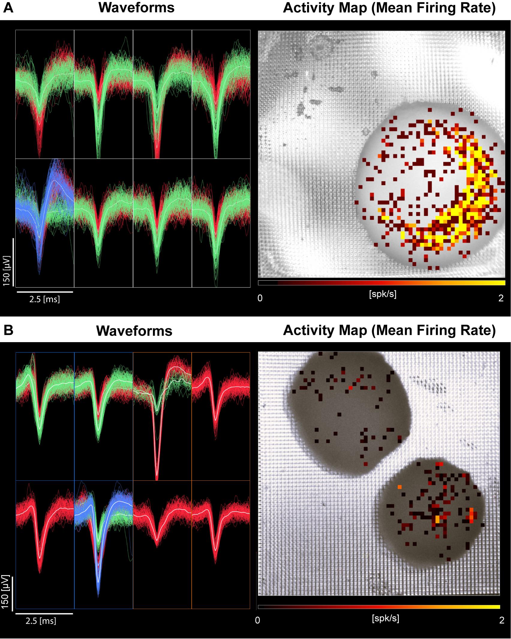
Figure 12. Recording of spontaneous activity in cortical and spinal cord organoids. (A) Representative spike waveforms (left) and corresponding activity map (right) from one cortical organoid (80 days in vitro). (B) Two spinal cord organoids (47 days in vitro) recorded simultaneously. Note that each box on the left side corresponds to waveforms from a single electrode. Color of the boxes (blue, orange) indicates organoid of origin, denoted on the activity map on the right side. For both panels, detected and sorted spikes are color-coded by unit number after spike sorting (red for neuron 1, green for neuron 2, blue for neuron 3). Activity maps on the right side show the mean firing rate per electrode (all neurons per electrode aggregated) in a 2 s integration window, overlaid on top of images showing organoid placement.
20. Use the Well Layers tool of BrainWave6 to overlay a high-resolution image of the 3D HD-MEA recording area. Make sure that all four corners of the electrode array are clearly visible in the image to ensure a perfect overlay.
21. Review the detected spikes and analysis outputs within the BrainWave6 interface.
Note: During initial data acquisition, BrainWave6 also generates a result data file containing spikes detected in real time (“on-the-fly” detection). These real-time detections are generated during recording and are not equivalent to batch-processed results. Batch processing applies the full spike detection workflow uniformly across the entire recording and provides more accurate and consistent spike detection than on-the-fly detection.
22. In the visualization selector menu, choose the desired visualization type. Examples: Waveforms, Activity Map, Raster Plot, Trend Chart, Box Plot, Violin Plot, Histogram Chart, Space-Time Activity Map, Bar Plot, Connectivity Graph, Center of Activity Trajectory, Spectrogram Plot, Power Spectrum Plot. Representative examples of waveforms and activity maps are shown in Figure 12.
23. Use the top toolbar to set metrics, regions to plot, display options, and axis fitting when applicable.
24. Open the Metric selector and choose a metric by first selecting its Data Type and then selecting the metric name.
Notes:
1. Reportable metrics include but are not limited to: Spikes [Number of Active Units, Number of Spikes, Mean Firing Rate, Inter-Spike Interval (ISI), ISI - CoV, Min Peak Amplitude (Abs value), Peak-to-Peak Amplitude]. Spike Network Bursts [Percentage of Spikes in Network Bursts, Inter-Network Burst Interval (INBI), INBI - CoV, Network Burst Peak, Time to Burst Peak, ISI - CoV within Network Burst, Mean ISI within Network Burst]. FP Network Bursts (IFPI - CoV within Network Burst, Mean IFPI within Network Burst, Median IFPI within Network Burst, Median/Mean IFPI within Network Burst, Network Burst IFPI - IQR, CAT Velocity, CAT Duration).
2. FP detection/analysis is typically not enabled for organoid recordings.
25. Use the Space Navigator panel to inspect the spatial distributions of detected activity.
26. Activity group–based filtering can be applied to restrict plots to units meeting an Activity Group definition or based on spatial subsets of the array. Alternatively, when multiple organoids are recorded simultaneously or when different regions occupy distinct areas of the electrode field, use the Zone tool to define regions of interest that follow the morphology of each organoid. This ensures that all the results are extracted independently for each sample.
27. After selecting the visualization type and specifying plotted data, use Chart Export to export either the plotted image or the underlying data.
Note: Exported CSV/Excel files from multiple recordings can be merged externally for downstream analysis.
C. General considerations
1. All recordings within an experiment are processed using an identical analysis workflow to ensure consistency.
2. Default BrainWave6 parameters from Spikes-3D Culture are used for most recordings. AI Validation is the main additional option enabled. Parameter testing and exploration are recommended to ensure settings match the dataset’s noise profile and experimental goals.
3. File naming conventions preserve traceability between raw recordings and processed outputs. Batch-processed .BXR results files are used for all downstream analyses unless otherwise stated.
Validation of protocol
This protocol has been used and validated in the following open-access research article:
Mapelli et al. [28]. Enhanced electrophysiological recordings in acute brain slices, spheroids, and organoids using 3D high-density multielectrode arrays. PLoS One 20(9): e0328903. https://doi.org/10.1371/journal.pone.0328903
In particular, see:
Figure 3A–C: A statistic on six cerebellar acute slices is reported for recordings using the 3D HD-MEA for the number of active electrodes, the number of recorded cells, the ratio of cells to electrode, the mean firing rate, and the peak-to-peak amplitude of the extracellular action potentials recorded.
Figure 4A–C: A statistic on three cortico-hippocampal acute slices for the number of cells recorded, the number of active electrodes, the number of spikes, and the peak-to-peak amplitude of the extracellular action potentials recorded.
Figure 5A–C: A statistic on 10 cerebellar acute slices for the time of action of tetrodotoxin (TTX, 3 μM) in suppressing neuronal firing.
Figure 7: A statistic on seven acute brain slices containing the prefrontal cortex is reported for the correlation index of the activity in the recorded channels in Krebs, mACSF, and after gabazine perfusion. Representative traces are reported here and in Supplementary Figure 4.
Figure 8: Quantification from the recordings of three spheroids of different sizes (large and small) in terms of number of electrodes sampling each spheroid, number of active electrodes, number of recorded cells, mean firing rate, peak-to-peak amplitude, and mean bursting rate.
Figures 9 and 10: Quantification from the recordings of two organoids, in terms of mean firing rate, burst frequency, and correlation analysis, including the pharmacological modulation of the organoid’s activity by varying KCl concentrations.
Supplementary Figure 1: Average of the activity recorded in five cerebellar acute slices over time, to quantify the recording stability.
Supplementary Figure 5: A statistic from seven acute brain slices containing the prefrontal cortex is reported for the basal firing rate and coefficient of variations (CV and CV2) in Krebs, mACSF, and during gabazine perfusion.
General notes and troubleshooting
General notes
1. Before starting any experiment, test the 3D HD-MEA to ensure its correct functioning. During this phase, culture media, Krebs, mACSF, or PBS can be used; no biological samples are required. To verify that the 3D HD-MEA is working correctly, open the Activity Map plot in the main window and display the standard deviation (SD) instead of the peak-to-peak amplitude. Place the mouse cursor over the map to display the “whole plate SD” value. Verify that the whole plate SD is ≤14 μV for a 100 Hz high-pass filter and ≤20 μV for a 5 Hz high-pass filter.
2. If multiple electrodes show high noise or a completely flat line, check Troubleshooting, problems 1–3.
3. To remove tissue from the 3D HD-MEA after an experiment:
a. Use a pair of fine tweezers or the holder handling tool to remove the sample holder insert from the sample holder frame.
Critical: Remove the sample holder insert perpendicularly; do not force it off.
b. Flush culture media, ACSF, or Krebs solution over the recording area to detach the tissue.
c. Discard the tissue.
d. If new samples are recorded, follow step 3e(i-iii) to remove any trapped cellular debris, then refill the 3D HD-MEA well to submerge the sample holder frame.
e. If the experimental session is concluded, clean the 3D HD-MEA as follows:
i. Fill the well with a 5% Extran enzymatic detergent solution in DDW.
ii. Flush the solution over the electrodes with a P1000 pipette for 1 min to create a thick foam.
iii. Rinse at least three times with DDW, flushing several times over the electrodes during each wash.
Critical: Ensure that all detergent is thoroughly removed to maintain the integrity of subsequent brain tissue.
iv. Let the 3D HD-MEA dry under a laminar hood before storing it in its box.
4. Following placement on the 3D HD-MEA, samples may benefit from a stabilization period prior to recording to allow recovery from handling, establishment of stable tissue–electrode coupling, and thermal equilibration. While an equilibration time of approximately 5 min is commonly sufficient, optimal timing may vary across preparations and should be validated empirically, particularly when balancing signal stability against experimental throughput. Of special consideration are organoids that are embedded in a hydrogel or other coating. It is recommended to equilibrate these organoids for a longer time, at least 10 min, to allow the electrodes to penetrate the organoid. Temperature is a critical variable, as neuronal firing rates and network properties are strongly temperature-dependent; consistent thermal conditions should therefore be maintained and verified throughout recordings.
5. 3D HD-MEA recordings from neural organoids are influenced by both biological and technical sources of variability. Standardization of the factors described below is critical for reproducibility and accurate interpretation of neuronal activity. Because the magnitude and direction of these effects can differ across differentiation protocols, genetic backgrounds, organoid models, and recording setups, users are encouraged to explicitly evaluate the contribution of each variable within their own experimental system rather than assuming uniform effects across models.
6. Neural organoids exhibit inherent heterogeneity in size, morphology, and cytoarchitecture, which can influence electrode coverage, signal amplitude, and the number of active channels detected. Neuronal excitability and network dynamics also change substantially over developmental time as synaptic connectivity and circuit organization mature. Consequently, the relationship between organoid age and electrophysiological output should be empirically characterized for each model system. Differences in cell-type composition, including the relative abundance of excitatory neurons, inhibitory interneurons, progenitors, and glial populations, further contribute to variability in baseline firing rates, bursting behavior, and network synchrony and should be considered when interpreting differences between organoids or experimental conditions. For example, we have recorded and detected active units in spinal cord organoids between 30 and 75 days in vitro and in cortical organoids between 43 and 210 days in vitro. The presence and frequency of spike bursts or spike network bursts can vary significantly across iPSC lines, organoid region types, batches, and recording conditions.
7. During 3D HD-MEA recordings, organoids remain metabolically active and are sensitive to environmental conditions. For short-duration recordings, standard culture media and ambient gas exchange are typically sufficient. For longer recordings or high-throughput experiments, CO2 supplementation (e.g., using the mini-incubator box) and adequate oxygenation should be considered to maintain physiological pH and tissue viability, as deviations in these parameters can alter neuronal excitability and network activity.
8. Technical factors related to the setup substantially influence recorded activity and may interact with biological variability. The inherent variability in microchip electronics may result in minor differences in sensitivity and noise characteristics across electrodes, and electrode performance can also change with repeated use of the same chip. However, when handled carefully, a chip can be reused for acute recordings dozens of times. Effective electrical coupling between the organoid and the electrode array depends on accurate positioning, the absence of air bubbles, and appropriate mechanical pressure applied via the organoid holder. Both insufficient and excessive pressure can distort recorded activity or compromise tissue viability; these parameters should therefore be evaluated systematically within each experimental setup.
9. Neural activity and signal stability may drift over the course of a recording session, highlighting the importance of standardizing recording duration and timing relative to the sample placement. To minimize technical variability when comparing experimental conditions, use the same 3D HD-MEA chip within an experiment whenever feasible. Overall, careful characterization and control of both biological and technical variables within each experimental system are essential for obtaining reproducible and interpretable 3D HD-MEA measurements.
10. Pharmacological interventions during recordings permit selective modulation of specific neuronal receptors, ion channels, or pathways, providing mechanistic insight into activity and excitability. To maintain stable recordings, the biological samples should remain fully covered, and medium volume should be standardized across wells. Drug application can be performed in two ways: (1) during an ongoing recording, where the time of addition is logged as an event in the 3Brain software, or (2) in a separate recording, where the drug-treated sample is recorded independently after baseline. Regardless of the method, it is important to consider the equilibration time required for each drug and experiment, and that the washout of pharmacological agents is challenging due to the difficulty of fully changing media without causing mechanical disruption. These factors should be considered when designing experiments.
Troubleshooting
Problem 1: One or more electrodes exhibit a high level of noise (std dev > 20 μV) in the recorded signal.
Possible cause: There are multiple possible causes for the aforementioned problem; the most common is the presence of air bubbles trapped on the sensing area of the electrodes due to high hydrophobicity. Another possible cause is the presence of debris or physical damage to the 3D electrodes.
Solution: Check the status of the electrodes by imaging the recording area with a stereo microscope or a high-resolution camera; if one or more electrodes are damaged or strongly bent, they cannot be restored. Thus, avoid placing the biological samples on top of those electrodes and remove them from the data analysis. If the high noise level is not caused by damaged electrodes, the cause might lie in the presence of debris if the chip has been previously used. In this case, fill the 3D HD-MEA well with an enzymatic detergent solution of 5% Extran in DDW and flush the solution for 1 min with a P1000 pipette to create a thick foam. Finally, rinse at least three times with DDW and flush several times on top of the electrodes during each wash. Then, add culture media, PBS, Krebs, or ACSF and test the 3D HD-MEA again. It is crucial to never touch the electrodes with the pipette tip to not damage them. If noise persists, it can still be caused by high hydrophobicity. In this case, first wet the electrode array with 70% EtOH and flush it for 1 min using a P1000 pipette. Then, rinse at least three times the 3D HD-MEA well with DDW by flushing several times on top of the electrodes during each wash. Then, add culture media, PBS, Krebs, or ACSF and test the 3D HD-MEA again.
Problem 2: All the electrodes are completely saturated, showing a flat voltage trace.
Possible cause: Air bubbles are trapped on one or both reference electrodes.
Solution: Use a P1000 pipette to flush the solution in the 3D HD-MEA well near the reference electrodes to remove any trapped bubbles. Alternatively, use a small soft paintbrush to dislodge and remove the bubbles from the recess around the reference electrodes.
Problem 3: One or more columns of electrodes are completely saturated, and the corresponding voltage traces show a flat line.
Possible cause: If there are 4 or multiples of 4 saturated columns spaced 16 electrodes apart, the cause of the issue lies in a poor electrical contact between the 3D HD-MEA and the BioCAM. In all other cases, the cause of the problem is mostly due to some damaged electrodes.
Solution: In case of poor electrical contact, proceed by cleaning the 3D HD-MEA golden contact pads with isopropanol. If the saturated columns result from damaged electrodes, these cannot be restored and should be excluded from data analysis.
Problem 4: The sample moved while placing the sample holder insert into the 3D HD-MEA well.
Possible cause: The sample holder insert moved too quickly during placement, resulting in liquid displacement that shifted the samples from their initial position.
Solution: Wait a few minutes before placing the sample holder insert to allow the sample to stabilize on the electrode array. Then, lower the sample holder insert gently when it is very close to the sample to minimize liquid displacement.
Problem 5: The sample holder insert does not move smoothly through the sample holder frame.
Possible cause: The sample holder silicone net is not positioned well into the sample holder insert. Some debris are preventing the movement of the sample holder insert.
Solution: Check that both ribs of the net are well inserted in the recess of the sample holder; if not, insert them properly. Check that no debris can prevent the movement of the sample holder insert; eventually, remove it with a paintbrush or tweezers.
Problem 6: The sample holder insert does not press evenly on the sample.
Possible cause: The sample holder silicone net is hydrophobic, and some air bubbles are trapped within the net holes. The sample holder silicone net is not perfectly parallel with the electrode array.
Solution: Before inserting the sample holder insert, place it in a Petri dish filled with PBS or cell media. With a P1000 pipette, flush the solution on top of the net to remove all air bubbles (Figure 13). If the net is still hydrophobic, 70% EtOH can be used to remove the bubbles. Then, wash the net with PBS or cell media before placing it into the 3D HD-MEA. If the net is not parallel with the electrode array, check that the net ribs are well inserted into the sample holder insert recess. Check also that the net is not deformed. If that is the case, replace the net with a new one.
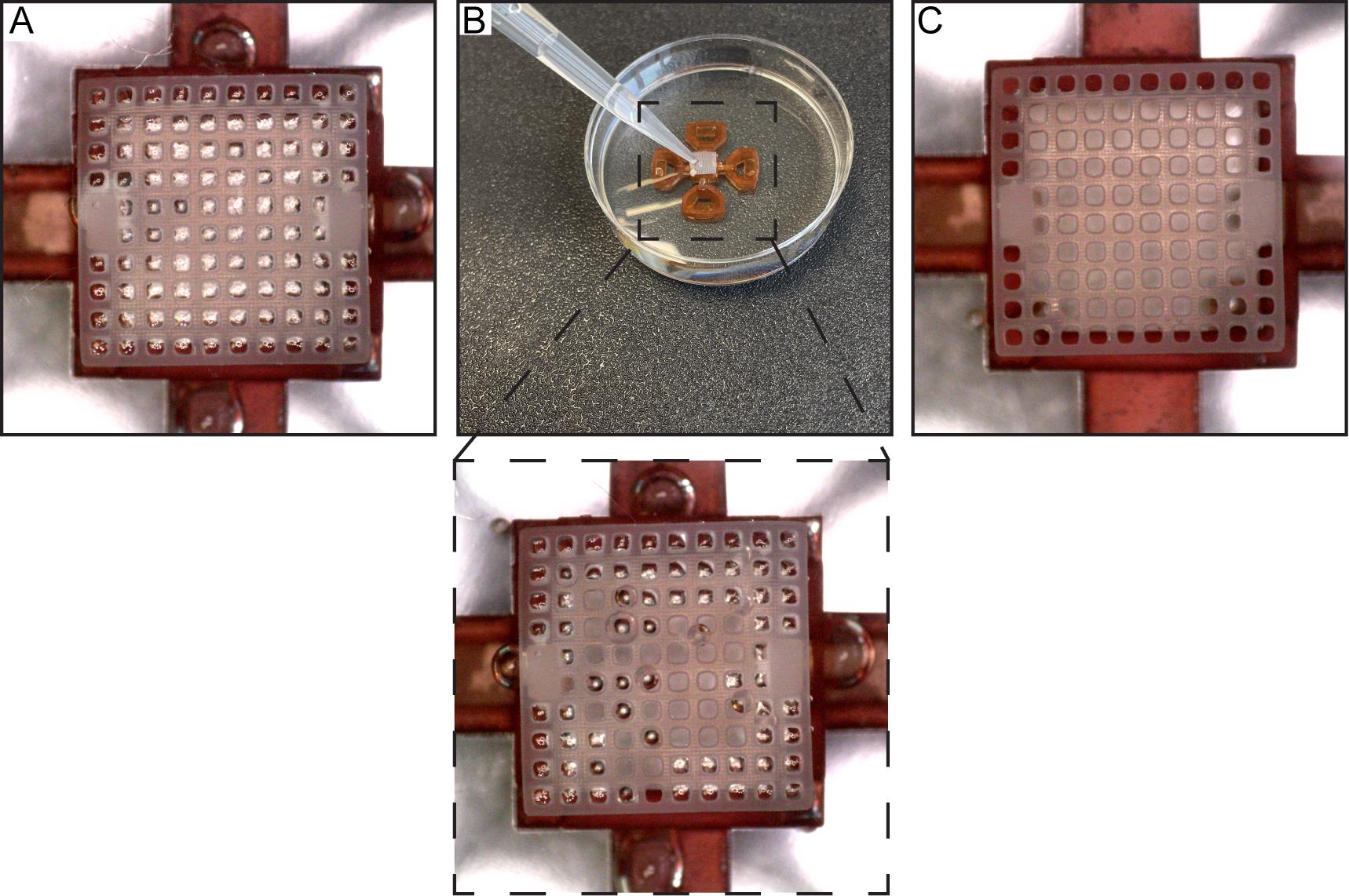
Figure 13. Removing air bubbles from the sample holder silicon net. (A) Image illustrating air bubbles trapped within the openings of the net. (B) Submerge the sample holder with the net into a 100 mm Petri dish filled with PBS. Using a P1000 pipette, repeatedly flush PBS over the net to dislodge and remove the trapped air bubbles (see inset). (C) Once all air bubbles have been completely removed, the sample holder insert can be placed into the sample holder frame.
Problem 7: Little or no detectable activity by visual inspection during recording.
Possible causes: Neuronal activity may be absent or below detection threshold, electrode–tissue contact may be insufficient, or the signal-to-noise ratio may be low, making activity difficult to discern prior to downstream analysis.
Solution: The sample may be repositioned on the 3D HD-MEA chip to improve electrode coverage and tissue contact. Increasing pressure using the appropriate sample holder insert can further enhance electrode coupling. Neuronal activity may also be evoked or unmasked through electrical stimulation or pharmacological intervention.
Problem 8: Spatially restricted activity detected on only a small subset of electrodes.
Possible causes: Neuronal activity may be localized to a specific region of the organoid that is preferentially in contact with the electrode array, while other regions remain electrically silent or too distant from the chip surface. Activity can often appear on the edges/circumference or the middle/bottom of the organoid.
Solution: Repositioning the organoid or performing multiple recordings with different orientations may be used to sample additional regions.
Problem 9: Active units detected in unexpected electrodes or regions of the 3D HD-MEA chip.
Possible causes: This may arise from noisy or damaged electrodes, detection of far-field spikes from neurons distant from the electrode(s), or electrical artifacts.
Solution: After Batch Processing, spurious or off-target spikes can be removed using the Event Post-Processing module in the Data Analysis tab. Filter the spikes to include only those from the selected Activity Group or electrodes of interest.
Acknowledgments
Conceptualization, L.M., A.M.; Writing—Original Draft, Review, Editing, E.P., G.P., M.C., L.M., A.M., G.S., I.V., F.M., A.A.S., and B.A.; Protocol Optimization, E.P., G.P., M.C., L.M., I.V., M.T., G.C., A.A.S., and B.A.; Data collection, E.P., G.P., M.C., G.S., I.V., F.M., S.S.W., and A.A.S.; Funding acquisition, L.M., E.D., A.M., F.B., J.A., and S.S.; Supervision, L.M., A.M, and E.D.
The authors acknowledge the #NEXTGENERATIONEU (NGEU) and Ministry of University and Research (MUR), National Recovery and Resilience Plan (NRRP), project MNESYS (PE0000006) – A Multiscale integrated approach to the study of the nervous system in health and disease (DN. 1553 11.10.2022) to E.D. This project has received funding from the European Union’s Horizon 2020 research and innovation program under the grant agreement 964877 – NEUCHIP to A.M. Work by M.C. was supported by the European Union’s Horizon Europe Programme under the Specific Grant Agreement No. 101147319 (EBRAINS 2.0 Project); work by E.P. and G.P. was supported by the European Union's Research and Innovation Program Horizon Europe under grant agreement No 101137289 (Virtual Brain Twin Project). The authors acknowledge the European Union – Next GenerationEU – National Recovery and Resilience Plan (NRRP) – Mission 4 Component 2 Investment 1.1 Call PRIN 2022 CUP F53D23005920006 (MUR code 20227JSRWB – Mechanisms of susceptibility to cortical spreading depression in migraine: a multiscale approach) to L.M. 3Brain AG provided support for this study in the form of salaries to M.T., G.S., C.R.B., M.G., K.I., and A.M. The specific roles of these authors are articulated above. The sponsors did not play any role in the design, data collection, analysis, decision to publish, or preparation of the manuscript.
This work was supported by grants from ALS Cure Project (J.A.), the ALS Association (J.A.; doi.org/10.52546/ALSA.24-SGP-690.pc.gr.187896), Edward Mallinckrodt Jr Foundation (J.A.), Tambourine’s ALS Breakthrough Research Fund in Partnership with the Milken Institute (J.A.), ALS Finding a Cure in Partnership with Hop on a Cure (J.A.), ADBDB Training Program (B.A.), and NIH F31 (NS139599) (A.A.S.).
This protocol was used in [28].
Competing interests
Mariateresa Tedesco, Giacomo Sciacca, Francesco Mainardi, Ivan Verduci, and Gendenver Cadiao are employees of 3Brain AG.
Alessandro Maccione is a shareholder of 3Brain AG.
The other authors declare that the research was conducted in the absence of any commercial or financial relationships that could be construed as a potential conflict of interest.
Ethical considerations
The generation of animal-derived spheroids was conducted by following experimental procedures and animal care complying with the European Communities Parliament and Council Directive of 22 September 2010 (2010/63/EU) and with the Italian D.L. n. 26/2014, and were approved by the Italian Ministry of Health (protocol number 75F11.N.6JI, 08/08/18). All possible efforts were made to minimize animal suffering and the number of animals used.
Human-derived spheroids and cortical organoids were generated by using commercial IPSC cell lines.
Human induced pluripotent stem cells and spinal cord organoids were generated following standardized experimental procedures, in compliance with policies outlined by the Emory School of Medicine institutional review board office.
Animal maintenance and experimental procedures used for acute slices were performed according to the international guidelines of the European Union Directive 2010/63/EU on the ethical use of animals and were approved by the local ethical committee of the University of Pavia (Italy) and by the Italian Ministry of Health (protocol authorized following art.1, comma 4 of the D.Lgs. n. 26/2014 and approved on December 9th, 2017; authorization n. 1019/2023-PR).
References
- Costamagna, G., Comi, G. Pietro and Corti, S. (2021). Advancing Drug Discovery for Neurological Disorders Using iPSC-Derived Neural Organoids. Int J Mol Sci. 22(5): 2659. https://doi.org/10.3390/ijms22052659
- Faravelli, I., Antón-Bolaños, N., Wei, A., Faits, T., Sampath Kumar, A., Andreadis, S., Kastli, R., Montero Crespo, M., Steiger, M., Leible, D., et al. (2025). Human brain organoids record the passage of time over multiple years in culture. bioRxiv. https://doi.org/10.1101/2025.10.01.679721
- Gordon, A., Yoon, S.-J., Tran, S. S., Makinson, C. D., Park, J. Y., Andersen, J., Valencia, A. M., Horvath, S., Xiao, X., Huguenard, J. R., et al. (2021). Long-term maturation of human cortical organoids matches key early postnatal transitions. Nat Neurosci. 24(3): 331–342. https://doi.org/10.1038/s41593-021-00802-y
- Imbriani, P., Sciamanna, G., Santoro, M., Schirinzi, T. and Pisani, A. (2018). Promising rodent models in Parkinson’s disease. Parkinsonism Relat Disord. 46: S10–S14. https://doi.org/10.1016/j.parkreldis.2017.07.027
- Mapelli, L., Soda, T., D’Angelo, E. and Prestori, F. (2022). The Cerebellar Involvement in Autism Spectrum Disorders: From the Social Brain to Mouse Models. Int J Mol Sci. 23(7): 3894. https://doi.org/10.3390/ijms23073894
- Andreatini, R. and Galduróz, J. C. F. (2026). Five proposals to increase translational value of animal models of neuropsychiatry disorders. Pharmacol Res Rep. 5: 100076. https://doi.org/10.1016/j.prerep.2026.100076
- Burns, T. C., Li, M. D., Mehta, S., Awad, A. J. and Morgan, A. A. (2015). Mouse models rarely mimic the transcriptome of human neurodegenerative diseases: A systematic bioinformatics-based critique of preclinical models. Eur J Pharmacol. 759: 101–117. https://doi.org/10.1016/j.ejphar.2015.03.021
- Zhao, X. and Bhattacharyya, A. (2018). Human Models Are Needed for Studying Human Neurodevelopmental Disorders. Am J Hum Genet. 103(6): 829–857. https://doi.org/10.1016/j.ajhg.2018.10.009
- de Leeuw, S. M., Davaz, S., Wanner, D., Milleret, V., Ehrbar, M., Gietl, A. and Tackenberg, C. (2021). Increased maturation of iPSC-derived neurons in a hydrogel-based 3D culture. J Neurosci Methods. 360: 109254. https://doi.org/10.1016/j.jneumeth.2021.109254
- Sloan, S. A., Darmanis, S., Huber, N., Khan, T. A., Birey, F., Caneda, C., Reimer, R., Quake, S. R., Barres, B. A. and Paşca, S. P. (2017). Human Astrocyte Maturation Captured in 3D Cerebral Cortical Spheroids Derived from Pluripotent Stem Cells. Neuron. 95(4): 779–790.e6. https://doi.org/10.1016/j.neuron.2017.07.035
- Andersen, J., Revah, O., Miura, Y., Thom, N., Amin, N. D., Kelley, K. W., Singh, M., Chen, X., Thete, M. V., Walczak, E. M., et al. (2020). Generation of Functional Human 3D Cortico-Motor Assembloids. Cell. 183(7): 1913–1929.e26. https://doi.org/10.1016/j.cell.2020.11.017
- Birey, F., Andersen, J., Makinson, C. D., Islam, S., Wei, W., Huber, N., Fan, H. C., Metzler, K. R. C., Panagiotakos, G., Thom, N., et al. (2017). Assembly of functionally integrated human forebrain spheroids. Nature. 545(7652): 54–59. https://doi.org/10.1038/nature22330
- Kiral, F. R., Cakir, B., Tanaka, Y., Kim, J., Yang, W. S., Wehbe, F., Kang, Y.-J., Zhong, M., Sancer, G., Lee, S.-H., et al. (2023). Generation of ventralized human thalamic organoids with thalamic reticular nucleus. Cell Stem Cell. 30(5): 677–688.e5. https://doi.org/10.1016/j.stem.2023.03.007
- Miura, Y., Li, M.-Y., Birey, F., Ikeda, K., Revah, O., Thete, M. V., Park, J.-Y., Puno, A., Lee, S. H., Porteus, M. H., et al. (2020). Generation of human striatal organoids and cortico-striatal assembloids from human pluripotent stem cells. Nat Biotechnol. 38(12): 1421–1430. https://doi.org/10.1038/s41587-020-00763-w
- Sloan, S. A., Andersen, J., Pașca, A. M., Birey, F. and Pașca, S. P. (2018). Generation and assembly of human brain region–specific three-dimensional cultures. Nat Protoc. 13(9): 2062–2085. https://doi.org/10.1038/s41596-018-0032-7
- Ballini, M., Muller, J., Livi, P., Chen, Y., Frey, U., Stettler, A., Shadmani, A., Viswam, V., Lloyd Jones, I., Jackel, D., et al. (2014). A 1024-Channel CMOS Microelectrode Array With 26,400 Electrodes for Recording and Stimulation of Electrogenic Cells In Vitro. IEEE J Solid-State Circuits. 49(11): 2705–2719. https://doi.org/10.1109/jssc.2014.2359219
- Berdondini, L., Bosca, A., Nieus, T. and Maccione, A. (2014). Active Pixel Sensor Multielectrode Array for High Spatiotemporal Resolution. In M. De Vittorio, L. Martiradonna, and J. Assad (Eds.), Nanotechnology and Neuroscience: Nano-electronic, Photonic and Mechanical Neuronal Interfacing (pp. 207–238). New York, NY: Springer New York. https://doi.org/10.1007/978-1-4899-8038-0_7
- Gagliano, G., Monteverdi, A., Casali, S., Laforenza, U., Gandini Wheeler-Kingshott, C. A. M., D’Angelo, E. and Mapelli, L. (2022). Non-Linear Frequency Dependence of Neurovascular Coupling in the Cerebellar Cortex Implies Vasodilation–Vasoconstriction Competition. Cells. 11(6): 1047. https://doi.org/10.3390/cells11061047
- González-Calvo, I., Iyer, K., Carquin, M., Khayachi, A., Giuliani, F. A., Sigoillot, S. M., Vincent, J., Séveno, M., Veleanu, M., Tahraoui, S., et al. (2021). Sushi domain-containing protein 4 controls synaptic plasticity and motor learning. eLife. 10: e65712. https://doi.org/10.7554/eLife.65712
- Hu, X., Khanzada, S., Klütsch, D., Calegari, F. and Amin, H. (2022). Implementation of biohybrid olfactory bulb on a high-density CMOS-chip to reveal large-scale spatiotemporal circuit information. Biosens Bioelectron. 198: 113834. https://doi.org/https://doi.org/10.1016/j.bios.2021.113834
- Monteverdi, A., Di Domenico, D., D’Angelo, E. and Mapelli, L. (2023). Anisotropy and Frequency Dependence of Signal Propagation in the Cerebellar Circuit Revealed by High-Density Multielectrode Array Recordings. Biomedicines. 11(5): 1475. https://doi.org/10.3390/biomedicines11051475
- Dorgau, B., Georgiou, M., Chaudhary, A., Moya-Molina, M., Collin, J., Queen, R., Hilgen, G., Davey, T., Hewitt, P., Schmitt, M., et al. (2022). Human Retinal Organoids Provide a Suitable Tool for Toxicological Investigations: A Comprehensive Validation Using Drugs and Compounds Affecting the Retina. Stem Cells Transl Med. 11(2): 159–177. https://doi.org/10.1093/stcltm/szab010
- Faravelli, I., Rinchetti, P., Tambalo, M., Simutin, I., Mapelli, L., Mancinelli, S., Miotto, M., Rizzuti, M., D’Angelo, A., Cordiglieri, C., et al. (2025). Targeted antisense oligonucleotide treatment rescues developmental alterations in spinal muscular atrophy organoids. Nat Commun. 17(1): 988. https://doi.org/10.1038/s41467-025-67725-1
- Paulsen, B., Velasco, S., Kedaigle, A. J., Pigoni, M., Quadrato, G., Deo, A. J., Adiconis, X., Uzquiano, A., Sartore, R., Yang, S. M., et al. (2022). Autism genes converge on asynchronous development of shared neuron classes. Nature. 602(7896): 268–273. https://doi.org/10.1038/s41586-021-04358-6
- Lancaster, M. A., Renner, M., Martin, C. A., Wenzel, D., Bicknell, L. S., Hurles, M. E., Homfray, T., Penninger, J. M., Jackson, A. P. and Knoblich, J. A. (2013). Cerebral organoids model human brain development and microcephaly. Nature. 501(7467): 373–379. https://doi.org/10.1038/nature12517
- Layrolle, P., Payoux, P. and Chavanas, S. (2022). Message in a Scaffold: Natural Biomaterials for Three-Dimensional (3D) Bioprinting of Human Brain Organoids. Biomolecules. 13(1): 25. https://doi.org/10.3390/biom13010025
- Pantula, A., Zhou, B., Morales Pantoja, I. E., Fedotova, A., George, D., Alam El Din, D.-M., Lysinger, A., Smirnova, L. and Gracias, D. H. (2025). Computational modeling of necrosis in neural organoids. bioRxiv. https://doi.org/10.1101/2025.04.30.651571
- Mapelli, L., Di Domenico, D., Sciacca, G., Mainardi, F., Ottaviani, A., Monteverdi, A., Tedesco, M., Battaglia, C. R., Tritto, S., Gandolfo, M., et al. (2025). Enhanced electrophysiological recordings in acute brain slices, spheroids, and organoids using 3D high-density multielectrode arrays. PLoS One. 20(9): e0328903. https://doi.org/10.1371/journal.pone.0328903
- Giza, J., Urbanski, M. J., Prestori, F., Bandyopadhyay, B., Yam, A., Friedrich, V., Kelley, K., D’Angelo, E. and Goldfarb, M. (2010). Behavioral and Cerebellar Transmission Deficits in Mice Lacking the Autism-Linked Gene Islet Brain-2. J Neurosci. 30(44): 14805–14816. https://doi.org/10.1523/JNEUROSCI.1161-10.2010
- Sanchez-Vives, M. V. and McCormick, D. A. (2000). Cellular and network mechanisms of rhythmic recurrent activity in neocortex. Nat Neurosci. 3(10): 1027–1034. https://doi.org/10.1038/79848
- Mainardi, F., Mapelli, L. and D’Angelo, E. (2024, October 9). HD-MEA NEUROPulse. Zenodo. https://doi.org/https://doi.org/10.5281/zenodo.13908319
- Hill, E. J., Sojka, C., Sampson, M. M., Kebede, N., Wang, H.-L. V., Showrin, S., King, A. T., Sing, A. D., Chang, J., Faundez, V., et al. (2026). Temporal regulation of human reactive astrocytes reveals their capacity for antigen presentation. Neuron. https://doi.org/10.1016/j.neuron.2026.02.025
- Sojka, C., Wang, H.-L. V., Bhatia, T. N., Li, Y., Chopra, P., Sing, A., Voss, A., King, A., Wang, F., Joseph, K., et al. (2025). Mapping the developmental trajectory of human astrocytes reveals divergence in glioblastoma. Nat Cell Biol. 27(2): 347–359. https://doi.org/10.1038/s41556-024-01583-9
- Voss, A. J., Lanjewar, S. N., Sampson, M. M., King, A., Hill, E. J., Sing, A., Sojka, C., Bhatia, T. N., Spangle, J. M. and Sloan, S. A. (2023). Identification of ligand–receptor pairs that drive human astrocyte development. Nat Neurosci. 26(8): 1339–1351. https://doi.org/10.1038/s41593-023-01375-8
- Tedesco, M. T., Di Lisa, D., Massobrio, P., Colistra, N., Pesce, M., Catelani, T., Dellacasa, E., Raiteri, R., Martinoia, S. and Pastorino, L. (2018). Soft chitosan microbeads scaffold for 3D functional neuronal networks. Biomaterials. 156: 159–171. https://doi.org/10.1016/j.biomaterials.2017.11.043
- Gibco by life technologies. (2013). Induction of Neural Stem Cells from Human Pluripotent Stem Cells Using PSC Neural Induction Medium (MAN0008031 Rev A.0). Retrieved from www.lifetechnologies.com/support
- Yoon, S.-J., Elahi, L. S., Pașca, A. M., Marton, R. M., Gordon, A., Revah, O., Miura, Y., Walczak, E. M., Holdgate, G. M., Fan, H. C., et al. (2019). Reliability of human cortical organoid generation. Nat Methods. 16(1): 75–78. https://doi.org/10.1038/s41592-018-0255-0
- Peters, C. E., Andersen, J., Li, M.-Y., Varanese, L., Thete, M. V., Yoon, S.-J., Pio, T., Thom, N., Chen, X., Qiao, W., et al. (2025). Human Assembloid Model of Emergent Neurotropic Enteroviruses. bioRxiv. https://doi.org/10.1101/2025.11.18.689148
- Maccione, A., Gandolfo, M., Massobrio, P., Novellino, A., Martinoia, S. and Chiappalone, M. (2009). A novel algorithm for precise identification of spikes in extracellularly recorded neuronal signals. J Neurosci Methods. 177(1): 241–249. https://doi.org/https://doi.org/10.1016/j.jneumeth.2008.09.026
Article Information
Publication history
Received: Feb 17, 2026
Accepted: Apr 23, 2026
Available online: May 14, 2026
Published: Jun 5, 2026
Copyright
© 2026 The Author(s); This is an open access article under the CC BY-NC license (https://creativecommons.org/licenses/by-nc/4.0/).
How to cite
Pali, E., Pellavio, G., Conforti, M., Sarkissian, A. A., Aliya, B., Sciacca, G., Wariyar, S. S., Mainardi, F., Tedesco, M., Verduci, I., Cadiao, G., Cervetto, C., Andersen, J., Birey, F., Maccione, A., D’Angelo, E. and Mapelli, L. (2026). Measuring Electrophysiological Activity in Acute Brain Slices, Spheroids, and Organoids Using 3D High-Density Multielectrode Arrays. Bio-protocol 16(11): e5708. DOI: 10.21769/BioProtoc.5708.

 Download Citation in RIS Format
Category
Neuroscience > Basic technology
Cell Biology > Tissue analysis > Electrophysiology
Cell Biology
Do you have any questions about this protocol?
Post your question to gather feedback from the community. We will also invite the authors of this article to respond.
 Post a Question


