


- Protocols

- Articles and Issues
- For Authors
- About
- Become a Reviewer


Analysis of Cauline Leaf Development in Arabidopsis thaliana Using Time-Lapse Confocal Microscopy

Published: Vol 16, Iss 10, May 20, 2026 DOI: 10.21769/BioProtoc.5691 Views: 520
Reviewed by: Pawan KumarAnonymous reviewer(s)
 PDF
PDF  Ask a question
Original research article
The authors used this protocol in:
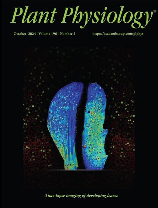
Aug 2024
Advertisement



Protocol Collections
Comprehensive collections of detailed, peer-reviewed protocols focusing on specific topics




Abstract
Understanding cellular growth dynamics in plants requires precise, long-term imaging of developing tissues. Cauline leaves are produced during the transition from vegetative to reproductive development and provide a useful system for studying how laminar organs diversify in form and function. While other laminar organs, such as rosette leaves and sepals, have been extensively studied, early cauline leaf development remains technically challenging to capture due to their concealed position, curved morphology, and the presence of dense trichomes. Here, we provide a complete pipeline for the dissection, confocal imaging, 2.5D segmentation, and image analysis of initiating cauline leaves in Arabidopsis thaliana. This method enables reproducible, high-resolution imaging of cauline leaves, supporting robust quantitative analysis of growth across developmental stages at cellular scale resolution.
Key features
• Fine dissection method for exposing initiating cauline leaves in Arabidopsis thaliana.
• Long-term confocal live imaging of cauline leaf development at cellular resolution.
• Optimized imaging parameters for high-fidelity 2.5D segmentation and growth analysis in MorphoGraphX.
Keywords: Confocal microscopy Live imaging
Cauline leaf
Growth dynamics
Image analysis
Organ development
Arabidopsis thaliana
Live imaging
Cauline leaf
Growth dynamics
Image analysis
Organ development
Arabidopsis thaliana
Graphical overview
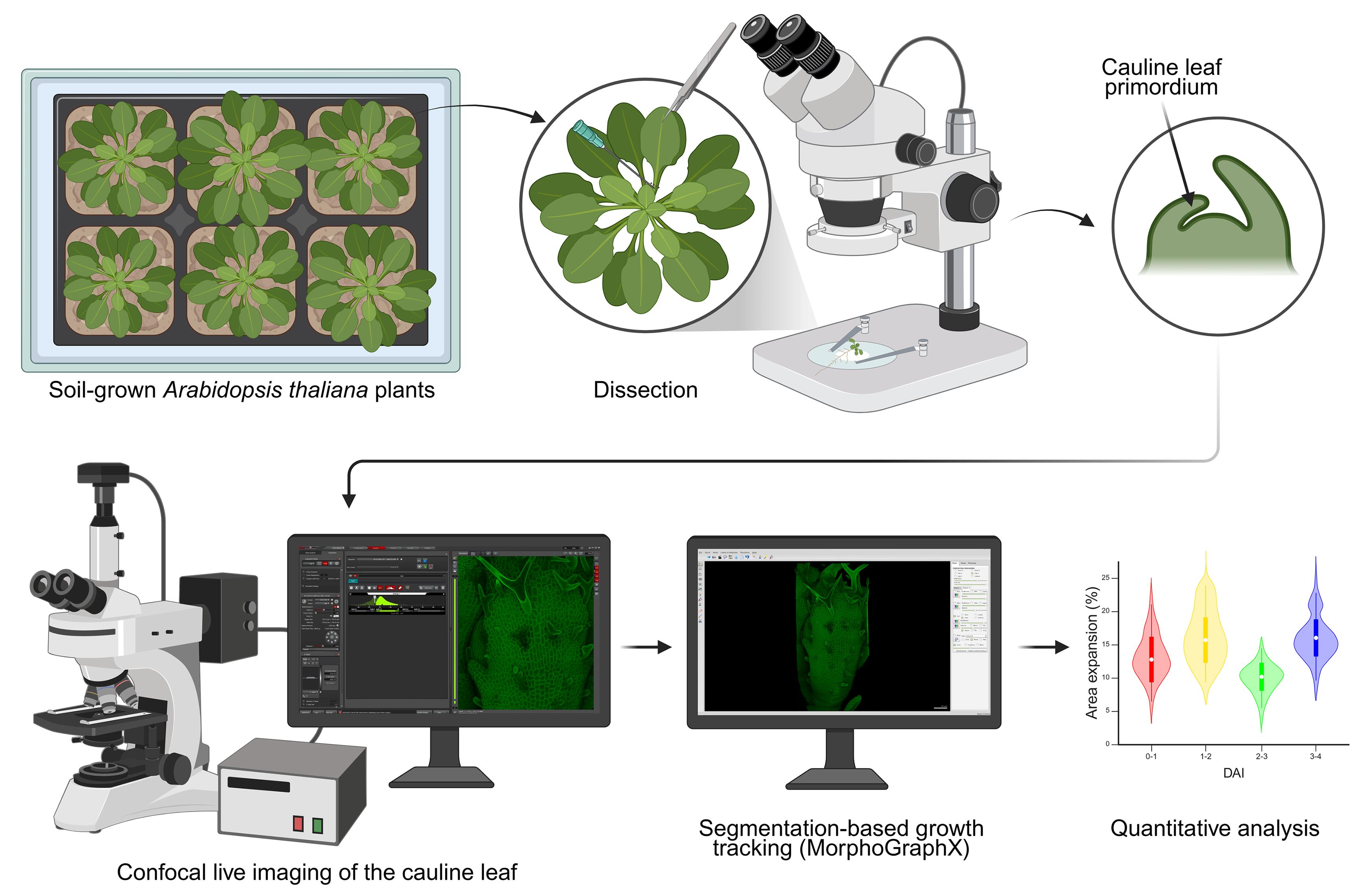
Workflow for long-term confocal imaging and growth tracking of cauline leaves. In the quantitative analysis step, area expansion refers to the increase in area of a cell lineage between successive time points; when a mother cell divides, the areas of the daughter cells are summed so that growth is quantified independently of cell division. Created in BioRender. Lab, M. (2026).
Background
Plant lateral organs, such as leaves and flowers, originate as simple protrusions at the shoot apical meristem but diversify greatly in size and shape to fulfill specific roles at maturity. While the developmental dynamics of rosette leaves and floral organs have been well characterized through live imaging and growth analysis, those of cauline leaves remain poorly understood [1–3].
Cauline leaves are initiated during the transition from vegetative to reproductive growth and combine characteristics of both rosette leaves and floral organs. They therefore provide a useful system for studying how developmental transitions reshape laminar organ identity, growth, and function. However, their early development is difficult to observe, as they are the last leaves to emerge from the meristem—prior to bolting and flower initiation—and are partially concealed by surrounding tissues. In addition, their pronounced curvature and dense trichome coverage on the abaxial surface make them challenging to image using existing approaches optimized for more accessible structures. Previous studies employing scanning electron microscopy or leaf removal have provided insights into morphology and developmental timing, but these techniques lack the spatial and temporal resolution required to capture dynamic growth processes [4–5].
In this paper, we present a protocol for confocal live imaging of initiating cauline leaves in Arabidopsis thaliana. We detail procedures for plant preparation, dissection, and long-term imaging of the same sample with minimal disruption to its development. The protocol is optimized for cellular-resolution imaging and subsequent quantitative analysis, including segmentation-based growth tracking. This method expands the live imaging toolkit to include a previously elusive organ type, enabling investigations into the cellular basis of heteroblasty and the developmental transitions underlying the diversification of laminar organs.
Materials and reagents
Note: The original workflow used in Le Gloanec et al. [6] was developed by the author at the University of Montreal, Canada. For the present protocol paper, the workflow was independently re-implemented at the National University of Singapore, Singapore, in order to validate reproducibility and to generate the illustrative material presented here. The illustrative images shown in this protocol were generated from the Singapore re-implementation, whereas the time-lapse datasets and macroscopic measurements used for validation are from Le Gloanec et al. [6]. This manuscript therefore presents the protocol in a stand-alone format, with expanded methodological detail, updated figures, and implementation notes from both locations. Where materials and reagents differed between the two locations, both versions are listed in the following sections, separated by “or.”
Biological materials
1. Arabidopsis thaliana Columbia-0 (Col-0) carrying the pUBQ10::myr:YFP construct, which encodes a plasma membrane-localized fluorescent marker, was used for time-lapse experiments [7]; other plasma membrane marker lines can also be used, like pUBQ10::PM-tdTomato [8] or p35S::LTI6b-GFP [9]
Reagents
1. ½ MS medium
a. Murashige and Skoog (MS) basal salt mixture (Sigma, catalog number: M552450L)
b. Murashige and Skoog (MS) vitamin solution (Sigma, catalog number: M3900-50ML)
c. Sucrose (Fisher, catalog number: S5-3)
d. Agar (Fisher, catalog number: BP1423-2)
or
a. Murashige and Skoog (MS) medium, including vitamins (Duchefa Biochemie, catalog number: M0222.0100)
b. MES monohydrate (Duchefa Biochemie, catalog number: M1503.1000)
c. Sucrose crystallized (Duchefa Biochemie, catalog number: S0809.5000)
d. Plant agar biotechnology grade (1st base, catalog number: 4020)
2. Plant preservative mixture (PPM) (Plant Cell Technology, catalog number: 71806-1)
3. 95% denaturated alcohol (Fisher, catalog number: HC-1100-1GL) or ethanol approx. 96% grade AR (QRëC, catalog number: E7045-1-2500)
Solutions
1. ½ MS medium (see Recipes)
2. 0.1% PPM solution (see Recipes)
3. 70% ethanol solution (see Recipes)
Recipes
1. ½ MS medium
| Recipe version 1 (Montreal) | Recipe version 2 (Singapore) |
|---|---|
| 2.15 g of MS basal salt mixture | 2.2 g of MS medium including vitamins |
| 10 g of sucrose | 10 g of sucrose crystallized |
| 1 mL of MS vitamin solution | 0.5 g of MES monohydrate |
| Add deionized H2O to 1 L | Add deionized H2O to 1 L |
| Adjust pH to 5.8 | Adjust pH to 5.8 |
| 15 g of agar | 15 g of plant agar |
| After autoclaving | |
| 1 mL of PPM | 1 mL of PPM |
2. 0.1% PPM immersion solution
1 L deionized H2O
1 mL of PPM
3. 70% ethanol solution
737 mL of 95% denatured alcohol
263 mL of sterile deionized H2O
Laboratory supplies
1. Plastic pots, trays, and lids for potting: thermoformed square pots with drainage 2.63” × 2.63” × 2.25”, no-hole trays 21” × 11” × 2.5”, and compatible plastic dome 21.50” × 11” × 2.10” (Teris) or thermoformed pots with drainage 95 × 78 × 75 mm, no-hole trays 54 × 28 × 6.5 cm, and compatible plastic domes 54 × 28 × 9 cm (Linyi Jiaxin Plastic Products Co., Ltd.)
2. All-purpose growing soil mixture (ASB Greenworld Grower Mix) or Jiffy FloraFleur potting soil M.70L/T002 (FarEastFlora, catalog number: 0000785)
3. 100 μL, 200 μL, and 1 mL pipettes with corresponding tips
4. 60 × 15 mm Petri dish (SARSTEDT, catalog number: 82.1194.500 or Corning®, catalog number: 430196)
5. Laboratory film (ParafilmTM)
6. Low lint tissue wipe (KimwipesTM, Kimberly-Clark)
7. Deionized H2O
8. Precision tweezers with fine point (Dumont No. 5)
9. Syringe needles, 18G × 1 1/2 and 27G × 1 1/2 (BD®, catalog number: 305196 and 301629)
10. Scalpel blades (FEATHER, #10)
11. Surgical tape (MicroporeTM tape 3M)
Equipment
1. Growth chamber, Conviron GEN1000 or Percival AR-66L3 with custom LED lighting (Grow Light C75 NS12, Valoya)
2. Autoclave
3. Laminar flow cabinet
4. Dissection stereomicroscope (Stemi 35, Zeiss or S8APO, Leica, equipped with KL 300 LED, Schott)
5. Upright confocal microscope equipped with long-working-distance water-dipping lenses (LSM800, Zeiss, with W Plan-Apochromat 40×/1.0 DIC M27 FWD = 2.5 mm or Stellaris 8 DM6 CFS, Leica, with HCX APO L 20×/1.0 W)
Software and datasets
1. Microscope software, Zeiss Zen 2.6 blue edition (Carl Zeiss Microscopy GmbH), or LAS X STELLARIS (Leica Microsystems)
2. MorphoGraphX 2.0.1 (https://morphographx.org/software/) (access date, 2026-02-26) [10–11]
3. All codes have been deposited to OSF: https://osf.io/uth78/ (access date, 2026-02-26)
Procedure
A. Plant growth
1. Sow the seeds in pots filled with moist, room-temperature soil. Add a layer of water to the bottom of the tray and cover with a lid to maintain high humidity.
Note: Space seeds sufficiently to avoid contact between the developing plants and to prevent leaf damage; typically, no more than four seeds per pot.
2. Stratify the sown seeds by placing the covered trays at 4 °C for two days.
Note: In our workflow, sowing before stratification helps maintain seed position and spacing in the pots while still providing uniform germination. Pre-stratification before sowing can also be used if preferred.
3. Transfer the trays to a growth chamber under long-day photoperiod conditions (16/8 h light/dark cycle, ~150 μmol.m-2.s-1), with 60%–70% relative humidity at 22 ± 1 °C. Water as needed.
Note: Avoid overwatering to minimize the risk of root anoxia and pest infestations. Proper watering supports healthy plant growth, which is essential for data reproducibility.
4. After approximately one week, or when the first two leaves are visible to the naked eye, begin gradually removing the plastic lid. Start by propping the lid ajar for a few days to help the plants acclimate to lower humidity levels before fully removing it.
B. Preparation of plates for imaging and plant culture
1. Prepare ½ MS medium (see Recipes) and autoclave at 121 °C for approximately 30 min.
Note: The sterilization time may vary depending on the autoclave model and load volume: adjust accordingly.
2. Allow the medium to cool to ~60 °C before adding PPM to the final concentration of 0.1% (v/v; see Recipes).
Note: PPM is a broad-spectrum biocide used to inhibit the germination of bacterial and fungal spores in plant tissue culture.
3. In a laminar flow cabinet, pour the medium into Petri dishes to fill them halfway. Allow the medium to solidify, then wrap the plates with Parafilm and store at 4 °C.
Note: Plates can be stored for up to three months if properly sealed and maintained under appropriate conditions.
C. Preparation of live imaging: dissection
1. Prepare the working space.
a. Clean all working surfaces and dissection tools (e.g., tweezers) using 70% ethanol (see Recipes).
b. Bring the ½ MS plates to room temperature.
c. Place a moistened Kimwipe on the stereomicroscope stage to prevent sample dehydration during dissection.
Note: Use deionized H2O to moisten the tissue wipe. Ensure it is damp but not overly saturated, as excessive moisture can make dissection difficult.
2. Select 2-week-old plants for dissection. Carefully remove each plant from the soil and gently rinse soil from the roots using a squeeze bottle of water (Figure 1A–C).
Note: Ensure the plants are well-watered prior to dissection, as turgid tissues are easier to handle and dissect cleanly.
3. Gently place the plant on the moistened Kimwipe (Figure 1D). Using tweezers, handle the plant carefully to avoid tissue damage. Position the plant horizontally so that the insertion points of the older leaves are clearly visible (Figure 1E).
Note: The older leaves can be used to handle the sample, minimizing the risk of damaging the root and hypocotyl, critical for plant survival.
4. Using an 18G injection needle for the earlier dissection steps and a 27G needle for the most delicate steps close to the meristem, carefully remove the older leaves by cutting them at their base (Figure 1F–G).
5. Once the younger leaves are exposed and the hypocotyl is visible, gently roll the plant using your finger instead of using the tweezers. Position the remaining oldest leaf so it faces sideways, then carefully cut it away.
Notes:
1. For easier handling and dissection, right-handed users should position the leaf to the right, and left-handed users to the left.
2. If there is a risk of damaging the sample, particularly when approaching the initiating cauline leaves and meristem, gently push the leaf tip outward to separate it from the internal organs and meristem before cutting with the needle.
6. Continue repeating the dissection steps until the oldest cauline leaf is exposed. This leaf is identifiable by its curvature toward the meristem and the presence of trichomes on its abaxial surface, while earlier-emerged adult leaves typically have trichomes on the adaxial surface (Figure 1H).
7. To remove the older cauline leaves, first orient the sample so that the base of the target leaf is clearly visible under the stereomicroscope. Then, using the needle tip, gently push the leaf blade outward to separate it from the inner organs and create space near the insertion point. Cut the leaf at its base using a shallow, controlled motion, taking care not to pull on the tissue or press toward the meristem. Repeat sequentially until the initiating primordium of the third cauline leaf is exposed.
Note: When working close to the meristem, proceed gradually. It is preferable to leave a small residual piece of an older leaf rather than risk damaging the primordium or shoot apex, provided that the remaining tissue does not obstruct the view of the leaf of interest.
8. Mount the sample into the ½ MS plate. Use a scalpel to cut a square chamber in the medium at the center of the plate, then make a slit perpendicular to one side of the chamber. Gently insert the root and hypocotyl into the slit, ensuring the primordium is oriented upward (Figure 1I–K).
Note: When repositioning the sample, handle the hypocotyl portion that is embedded in the medium to rotate the entire sample and align the cauline leaf primordium to the microscope objective.
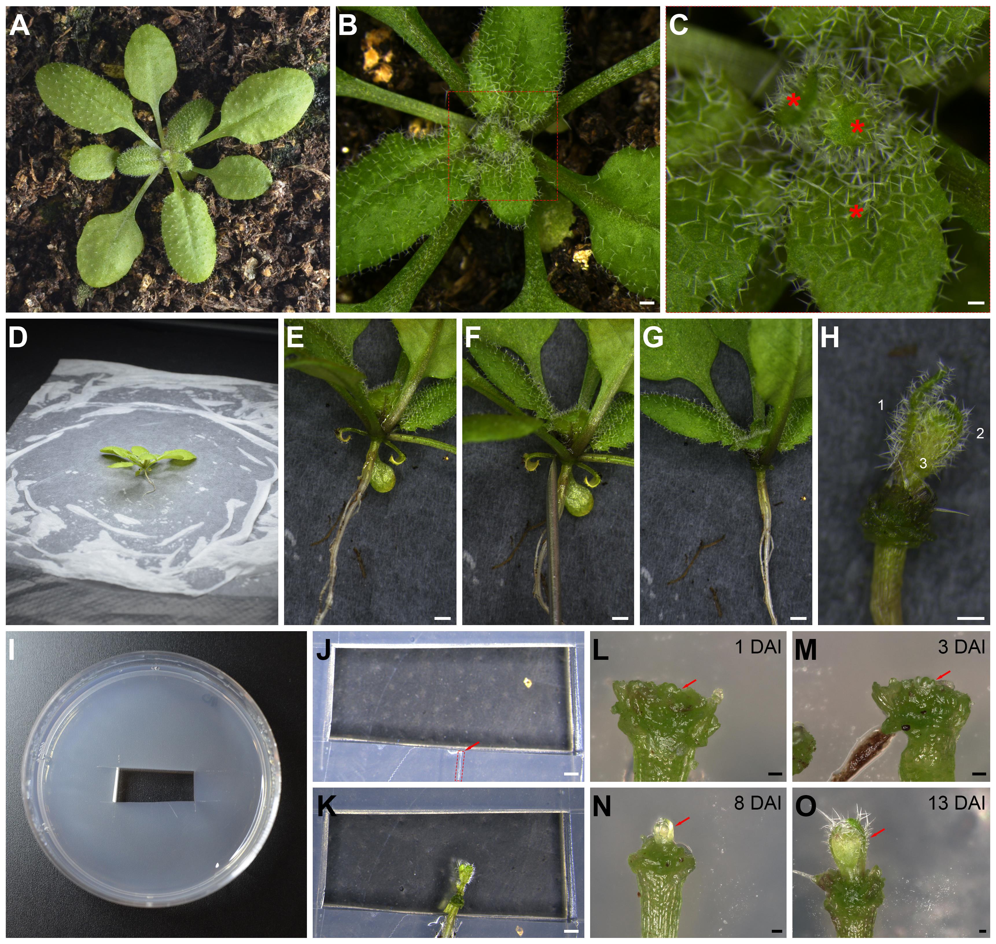
Figure 1. Experimental procedure for cauline leaf dissection in Arabidopsis thaliana. (A) Two-week-old plants are selected. (B, C) The plant shown for illustration already has the first two cauline leaves developed, identifiable by trichomes on their adaxial surfaces (red stars). The aim of this protocol is to expose the cauline leaf primordia and floral organs hidden beneath older leaves. (D) The rinsed plant is placed on a moistened Kimwipe under the dissection stereomicroscope. (E–H) The plant is positioned on its side by holding the older leaves (E), and an injection needle (F) is used to remove older leaves sequentially (G) until the first cauline leaf is exposed (cauline leaf 1, H). In panel H, numbers 1, 2, and 3 indicate the first, second, and third cauline leaves, respectively. (I–K) A square chamber and a slit (arrow and box in J) are cut into a ½ MS plate (I, J), and the sample hypocotyl is inserted into the slit (K). (L–O) Examples of dissected samples at different stages: 1 DAI (L), 3 DAI (M), 8 DAI (N), and 13 DAI (O). Arrows indicate the cauline leaf in each panel, numbers indicate the cauline leaf stage. DAI, days after initiation of the cauline leaf. Scale bars: 100 μm (L–O), 200 μm (C), 500 μm (B, H), and 1 mm (E–G, J–K).
D. Confocal imaging
1. Fill the plate with 0.1% PPM immersion solution (see Recipes), ensuring that the samples are completely submerged (Figure 2A).
Notes:
1. Check the position of the sample under the stereomicroscope after immersion and adjust if necessary.
2. Ensure that no air bubbles are present on the surface of the sample. If bubbles are observed, use a low volume (e.g., 100 or 200 µm) pipette, positioning the tip near the bubble, and pipette gently to remove it. Take care not to disturb the sample.
c. Allow the plate to sit for a few minutes to ensure both the sample and medium stabilize in the imaging solution. Differences in osmolarity may cause tissue or agar expansion and sample displacement during scanning, which is particularly critical when acquiring multiple tile scans for samples larger than the field of view (see step D5).
2. Place the plate on the microscope stage, secure it using the plate holder, and align the sample and the objective (Figure 2 A–B).
Critical: Refer to General note 1 to determine how to optimally set the confocal settings.
3. Once confocal settings are finalized, begin imaging the cauline leaves expressing the plasma membrane marker.
Note: Aim for a minimum of three biological replicates (individual plants) per developmental stage to ensure robust statistical analysis. Samples imaged at earlier stages can be included in later-stage series by aligning them based on cauline leaf size and morphology.
4. Once the image stack is acquired, use the 3D display tool of the microscope software to verify image quality. Ensure there are no signs of deformation caused by vibrations, sample drift, or movement during acquisition.
Note: Always ensure that the antivibration table on which the microscope is installed is turned on before imaging to minimize artifacts caused by motion and preserve image quality.
5. For samples larger than the field of view, acquire multiple overlapping image stacks. Begin scanning from one end of the sample, ensuring complete coverage along the mediolateral axis before progressing along the proximodistal axis (Figure 2D).
Note: After acquisition, load the image tiles into MorphoGraphX for preliminary stitching to verify if the entire sample has been imaged.
6. When imaging is complete, remove the plate from the microscope stage and discard the PPM solution.
Critical: The presence of excess liquid in the plate will impair sample growth. Carefully remove any remaining liquid using a Kimwipe, taking care not to touch or disturb the sample.
7. Before bringing the sample on the plate back to the growth chamber, verify that the sample is positioned in such a way that allows unidirectional, upright shoot growth. For example, if the plate is to be kept vertical, ensure the sample can be aligned to the light source and opposite to the direction of gravity by tilting the plate. Reposition the sample if necessary.
Note: For long-term experiments, transfer the sample to a fresh plate approximately every five days to ensure adequate nutrient availability and to minimize the risk of contamination. Under these conditions, contamination was infrequent in our hands when sterile plate preparation, PPM supplementation, and periodic transfer to fresh plates were maintained.
8. Seal the plate with Micropore tape and place it in a growth cabinet set to the same environmental conditions as the original growth chamber used for plant cultivation (Figure 2C).
9. After the defined time interval (e.g., 12 or 24 h), restart the protocol from step D1.
10. For datasets intended for 2.5D segmentation and growth quantification, keep acquisition parameters such as bit depth, z-step size, tile overlap, and signal level as consistent as possible across samples and time points, as these directly affect segmentation quality and downstream measurements.
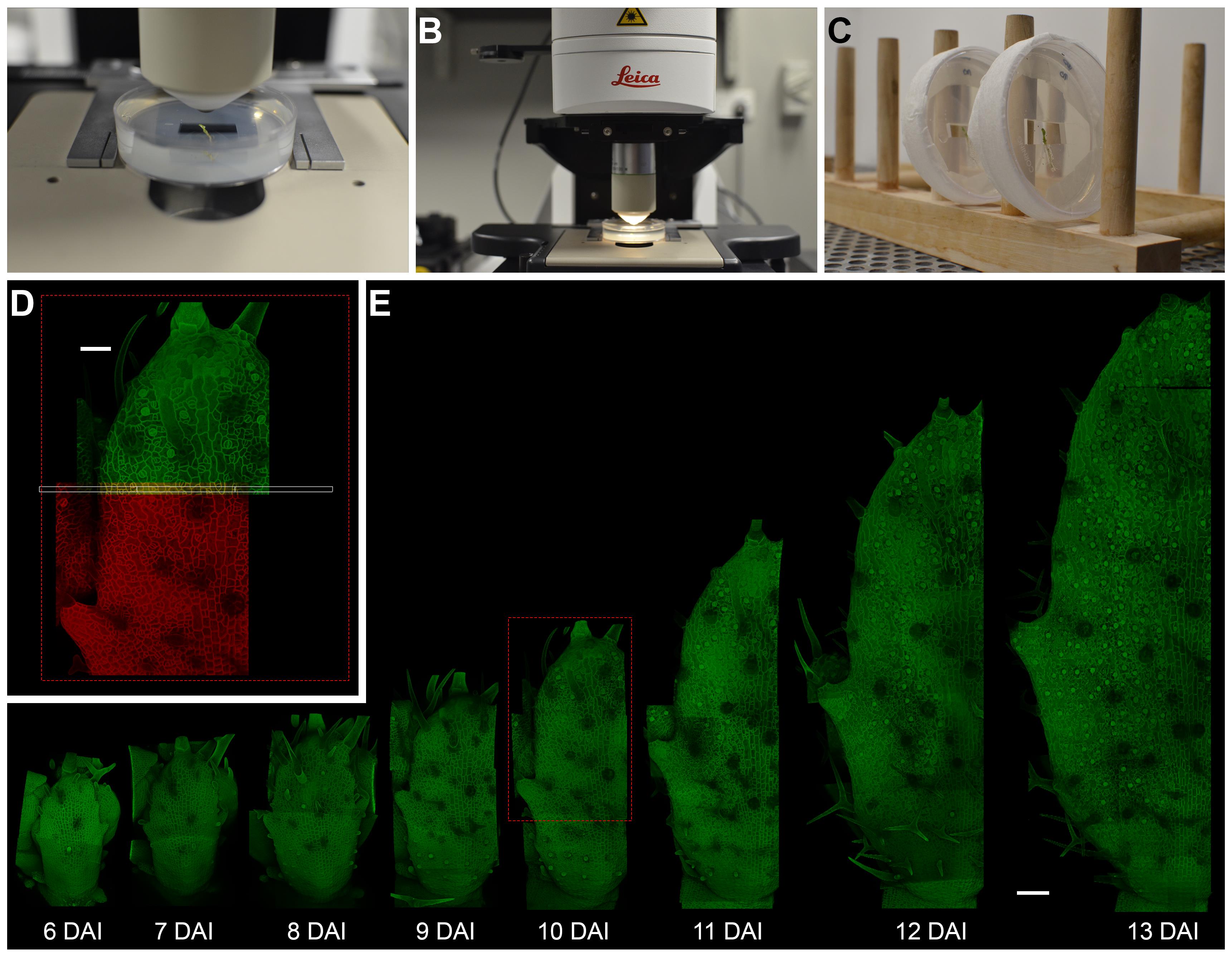
Figure 2. Confocal imaging of the Arabidopsis thaliana cauline leaf. (A, B) The sample is immersed in 0.1% PPM solution and placed on the confocal microscope for imaging. (C) After imaging, the sample is returned to the growth cabinet until the next time point, keeping it upright to allow for unidirectional growth. (D) For samples larger than the field of view, multiple tiles are acquired and stitched in MorphoGraphX. (E) Time-lapse series showing cauline leaf development from 6 to 13 DAI. DAI, days after initiation of the cauline leaf. Scale bars: 50 μm (D), 100 μm (E).
Data analysis
Notes:
1. Consistent naming conventions within the dataset are essential for the proper execution of scripts used for plotting and analysis.
2. Data obtained from this protocol can be used for 2.5D cell segmentation and growth quantification using the image analysis software MorphoGraphX. Images were processed and analyzed as described previously [6,10]. Scripts used for data analysis and plot generation are available at https://osf.io/uth78/ and are written in R or Python.
1. Import the confocal image stacks into MorphoGraphX. Image stacks must first be converted from the native microscope file format to .tif format (e.g., .lif for Leica or .czi for Zeiss). If multiple overlapping stacks were acquired, begin by stitching them to obtain a single image volume for downstream analysis (Figure 2D).
2. Blur the stack using Gaussian blur with a value of 0.3, then detect the organ surface using the Edge detect function. Adjust the threshold empirically according to sample quality and signal intensity. If the threshold is too high, holes may form in the detected surface; if it is too low, spikes may appear. For 2.5D segmentation, only the base of the trichome is relevant. Trichomes can therefore be virtually removed using clipping planes and the Voxel edit tool while moving through the organ. To improve surface detection near the organ margins, use Edge detect angle after creating the original global object and removing the trichomes. Before this step, rotate the object as needed without changing its axis. The value used for Edge detect angle is typically about half that used for Edge detect. If small holes remain at the surface, the Closing tool can be used; a radius of 3–5 is usually sufficient. If larger corrections are required, it is preferable to repeat the surface detection step with adjusted parameters.
3. Generate the surface mesh using Marching cubes surface with a cube size of 5 μm. Trim the bottom of the mesh, then iteratively subdivide and smooth it until a sufficiently smoothed surface is obtained. In practice, the mesh can be subdivided and smoothed sequentially, with additional local smoothing used to correct small imperfections when needed. For optimal performance during segmentation, keep the mesh below approximately 7 million triangles. Use clipping planes to verify how closely the generated surface matches the original image stack.
4. Project the membrane signal onto the surface mesh. A projection interval of approximately 2 μm is often suitable, as this corresponds roughly to the thickness of a cell wall. Adjust the start and end depths of the projection according to image quality, signal intensity, and the accuracy of the surface mesh to obtain the clearest membrane signal.
5. Perform cell segmentation by manually placing seeds within the outline of the cells using the New seed tool and then applying Watershed segmentation to propagate the seeds. Compare the resulting segmentation with the projected membrane signal and manually correct any errors where needed before proceeding to downstream analysis.
6. Perform lineage tracing (parenting) by loading the first time point as mesh 1 and the second time point as mesh 2. In mesh 2, tick the Parent box. Transfer the labels from mesh 1 to mesh 2, then use Check correspondence to verify that the parent-daughter relationships are correct. Manually correct any errors where needed.
7. Annotate cell types and zones if needed. Select the cells of interest and assign a specific parent label to the entire group. For example, stomata can be assigned label 16 and displayed in red. Apply the same approach consistently to define other cell types or spatial zones of interest.
8. Generate heat maps and export quantitative data for the parameters of interest as .csv files. These files can then be used as input for the custom R or Python scripts deposited on OSF for downstream data analysis and plot generation.
Validation of protocol
This protocol has been used and validated in the following research article:
Le Gloanec et al. [6]. Modulation of cell differentiation and growth underlies the shift from bud protection to light capture in cauline leaves. Plant Physiology.
The time-lapse datasets and macroscopic measurements used for validation are reported in that study.
General notes and troubleshooting
1. Prior to imaging, it is essential to optimize the confocal settings to ensure reliable data acquisition for downstream cell segmentation and growth quantification using the software MorphoGraphX. Once confirmed, the same settings should be maintained across all samples and time points for consistency.
a. Objective selection: For our experiments, we used a long-working-distance water-dipping W Plan-Apochromat 40×/1.0 objective (Zeiss). Other water-dipping objectives with different magnifications may be used, provided the numerical aperture (NA) is ≥0.8. For illustrative purposes in this protocol, a 20×/1.0 water-immersion objective (Leica) was used.
b. Fluorophore excitation and emission settings: Configure excitation and detection ranges according to the fluorophore(s) used and the specifications of your microscope (available laser lines, detectors, and filter/spectral settings). For the plasma membrane marker used in [6], YFP was excited at 488 nm, and emission was collected between 500 and 550 nm. YFP is also commonly excited using a 514-nm laser line on systems that provide it, with an emission window adjusted accordingly. The settings used in [6] were optimized for the imaging system in Montreal and may not be directly transferable. Therefore, determine excitation and detection ranges for your own fluorophore(s) and imaging system.
Note: When imaging multiple fluorophores simultaneously, adjust detection channels to minimize spectral overlap and bleed-through while maintaining optimal signal intensity. For red fluorophores or stains, optimize the emission detection range to reduce interference from chlorophyll autofluorescence, which emits strongly in the red and far-red regions.
c. Signal optimization: After locating and focusing on the sample, activate live mode to adjust gain and laser power for optimal visualization of cell outlines. Because absolute laser output and displayed percentage values vary between microscope systems and acquisition modes, no universal laser percentage is recommended. Instead, begin with the lowest laser power that still provides a sufficiently clear membrane signal for segmentation, and only increase as needed. In our hands, imaging was typically performed at low laser power settings, for example around 4% on a Leica system operated in counting mode. Similar low-percentage settings were used on the Zeiss system operated in analog mode, but these values are provided as instrument-specific examples and must be re-optimized locally.
Notes:
1. For accurate cell segmentation, a strong signal at cell boundaries is essential. Use the range indicator tool to slightly oversaturate epidermal layer pixels by adjusting laser power and master gain. Compensate for signal attenuation when scanning deeper into the tissue, if needed.
2. If the experiment involves quantifying fluorescence intensity, avoid saturating the signal or adjusting laser and gain while scanning.
Critical: High laser intensity can cause phototoxicity, including photobleaching and oxidative stress, which may inhibit growth or damage the tissue. Carefully balance image quality with the laser tolerance of the sample.
d. Bit depth: Acquire images in 16-bit format to enhance signal resolution and improve contrast between cell interiors and membranes.
e. Z-step size: Use a small Z-step to improve resolution in the Z-axis. For optimal results, the voxel dimension in x, y, and z should be as close to cubic as possible.
Note: A Z-step size of ≤ 1 µm is recommended, depending on the specific analysis planned.
2. Dissection, laser exposure, and in vitro growth conditions can induce stress in the sample. As a result, growth may appear slow during the first one or two time points. This does not necessarily indicate the sample has died, especially when imaging cauline leaves beyond the earliest developmental stages, where a brief slow-growth phase is expected. Allow additional time for recovery. However, if growth remains stagnant over several time points with no visible cell divisions, it is likely that the sample has ceased developing and should be discarded. To increase the chances of obtaining viable time series, we recommend dissecting multiple samples in parallel. Imaging series can also be overlapped to ensure continuous coverage of key developmental stages.
3. It can sometimes be challenging to determine whether a primordium is a cauline leaf or an adult leaf, even when counting the number of leaves. If uncertain, allow a couple of days for observation to see which side the trichomes form on, as this can help distinguish the organ type. If it turns out that the primordium is not the third cauline leaf, the sample can be redissected or reoriented to ensure proper imaging of the correct organ.
4. Due to their bilateral symmetry, imaging only half of a cauline leaf is often sufficient for downstream analysis. This reduces acquisition time and minimizes laser exposure, helping to preserve sample health throughout long-term imaging sessions.
Acknowledgments
I thank Pr. Yuchen Long and Dr. Andrea Gómez-Felipe for the critical reading of the manuscript.
This work was supported by Discovery grants (RGPIN-2018-05762 and RGPIN-2018-04897) from the Natural Sciences and Engineering Research Council of Canada, as well as a Team Grant from the Fonds de Recherche du Québec Nature et Technologies (2021-PR-282285). CLG was further supported by a Singapore Ministry of Education Academic Research Fund Tier 2 grant (MOE AcRF T2EP30122-0033).
This protocol was prepared from the workflow originally used in Le Gloanec et al. [6] and expanded into a stand-alone protocol, including updated methodological descriptions, revised figures, and reproducibility notes based on implementation in Montreal and Singapore.
The following figure was created using BioRender: Graphical overview, BioRender.com/vgxnefd.
Competing interests
The author declares no conflicts of interest.
References
- Hervieux, N., Dumond, M., Sapala, A., Routier-Kierzkowska, A. L., Kierzkowski, D., Roeder, A. H., Smith, R. S., Boudaoud, A. and Hamant, O. (2016). A Mechanical Feedback Restricts Sepal Growth and Shape in Arabidopsis. Curr Biol. 26(8): 1019–1028. https://doi.org/10.1016/j.cub.2016.03.004
- Echevin, E., Le Gloanec, C., Skowrońska, N., Routier-Kierzkowska, A. L., Burian, A. and Kierzkowski, D. (2019). Growth and biomechanics of shoot organs. J Exp Bot. 70(14): 3573–3585. https://doi.org/10.1093/jxb/erz205
- Kierzkowski, D., Runions, A., Vuolo, F., Strauss, S., Lymbouridou, R., Routier-Kierzkowska, A. L., Wilson-Sánchez, D., Jenke, H., Galinha, C., Mosca, G., et al. (2019). A Growth-Based Framework for Leaf Shape Development and Diversity. Cell. 177(6): 1405–1418.e17. https://doi.org/10.1016/j.cell.2019.05.011
- Pabón‐Mora, N., Sharma, B., Holappa, L. D., Kramer, E. M. and Litt, A. (2013). The Aquilegia FRUITFULL‐like genes play key roles in leaf morphogenesis and inflorescence development. Plant J. 74(2): 197–212. https://doi.org/10.1111/tpj.12113
- Ding, M., Zhu, Y. and Kinoshita, T. (2022). Stomatal properties of Arabidopsis cauline and rice flag leaves and their contributions to seed production and grain yield. J Exp Bot. 74(6): 1957–1973. https://doi.org/10.1093/jxb/erac492
- Le Gloanec, C., Gómez-Felipe, A., Alimchandani, V., Branchini, E., Bauer, A., Routier-Kierzkowska, A. L. and Kierzkowski, D. (2024). Modulation of cell differentiation and growth underlies the shift from bud protection to light capture in cauline leaves. Plant Physiol. 196(2): 1214–1230. https://doi.org/10.1093/plphys/kiae408
- Willis, L., Refahi, Y., Wightman, R., Landrein, B., Teles, J., Huang, K. C., Meyerowitz, E. M. and Jönsson, H. (2016). Cell size and growth regulation in the Arabidopsis thaliana apical stem cell niche. Proc Natl Acad Sci USA. 113(51): e1616768113. https://doi.org/10.1073/pnas.1616768113
- Melnyk, C. W., Schuster, C., Leyser, O. and Meyerowitz, E. M. (2015). A Developmental Framework for Graft Formation and Vascular Reconnection in Arabidopsis thaliana. Curr Biol. 25(10): 1306–1318. https://doi.org/10.1016/j.cub.2015.03.032
- Hamant, O., Heisler, M. G., Jönsson, H., Krupinski, P., Uyttewaal, M., Bokov, P., Corson, F., Sahlin, P., Boudaoud, A., Meyerowitz, E. M., et al. (2008). Developmental Patterning by Mechanical Signals in Arabidopsis. Science. 322(5908): 1650–1655. https://doi.org/10.1126/science.1165594
- Barbier de Reuille, P., Routier-Kierzkowska, A. L., Kierzkowski, D., Bassel, G. W., Schüpbach, T., Tauriello, G., Bajpai, N., Strauss, S., Weber, A., Kiss, A., et al. (2015). MorphoGraphX: A platform for quantifying morphogenesis in 4D. eLife. 4: e05864. https://doi.org/10.7554/elife.05864
- Strauss, S., Runions, A., Lane, B., Eschweiler, D., Bajpai, N., Trozzi, N., Routier-Kierzkowska, A. L., Yoshida, S., Rodrigues da Silveira, S., Vijayan, A., et al. (2022). Using positional information to provide context for biological image analysis with MorphoGraphX 2.0. eLife. 11: e72601. https://doi.org/10.7554/elife.72601
- Le Gloanec, C., Collet, L., Silveira, S. R., Wang, B., Routier-Kierzkowska, A. L. and Kierzkowski, D. (2022). Cell type-specific dynamics underlie cellular growth variability in plants. Development. 149(14): e200783. https://doi.org/10.1242/dev.200783
Article Information
Publication history
Received: Feb 27, 2026
Accepted: Apr 10, 2026
Available online: Apr 27, 2026
Published: May 20, 2026
Copyright
© 2026 The Author(s); This is an open access article under the CC BY-NC license (https://creativecommons.org/licenses/by-nc/4.0/).
How to cite
Readers should cite both the Bio-protocol article and the original research article where this protocol was used:
- Le Gloanec, C. (2026). Analysis of Cauline Leaf Development in Arabidopsis thaliana Using Time-Lapse Confocal Microscopy. Bio-protocol 16(10): e5691. DOI: 10.21769/BioProtoc.5691.
- Le Gloanec, C., Gómez-Felipe, A., Alimchandani, V., Branchini, E., Bauer, A., Routier-Kierzkowska, A. L. and Kierzkowski, D. (2024). Modulation of cell differentiation and growth underlies the shift from bud protection to light capture in cauline leaves. Plant Physiol. 196(2): 1214–1230. https://doi.org/10.1093/plphys/kiae408

 Download Citation in RIS Format
Category
Plant Science > Plant developmental biology > Morphogenesis
Cell Biology > Cell imaging > Confocal microscopy
Plant Science > Plant cell biology > Cell imaging
Do you have any questions about this protocol?
Post your question to gather feedback from the community. We will also invite the authors of this article to respond.
 Post a Question


