


- Protocols

- Articles and Issues
- For Authors
- About
- Become a Reviewer


Limited Proteolysis Mass Spectrometry to Identify Protein Structural Differences in Brain Tissue

Published: Vol 16, Iss 9, May 5, 2026 DOI: 10.21769/BioProtoc.5670 Views: 1061
Reviewed by: Ting MiaoDhananjay D ShindeElena A. Ostrakhovitch
 PDF
PDF  Ask a question
Original research article
The authors used this protocol in:

Jul 2025
Advertisement



Protocol Collections
Comprehensive collections of detailed, peer-reviewed protocols focusing on specific topics




Related protocols
Abstract
Structural proteomics methods allow for the proteome-wide interrogation of protein structural differences between two different conditions. Limited proteolysis mass spectrometry (LiP-MS), as originally implemented by the Picotti lab, utilizes a promiscuous protease to cleave at solvent-exposed regions of a protein to encode structural information, which is then read out with mass spectrometry proteomics. Here, we present a protocol that details experimental steps and data analysis for a LiP-MS workflow. First, tissue is homogenized under native conditions and then subjected to limited proteolysis using proteinase K (PK). The samples are prepared for mass spectrometry, and data are acquired using either data-dependent acquisition (DDA) or data-independent acquisition (DIA). Raw data is processed using FragPipe, and raw ion abundances are processed in FragPipe Limited-Proteolysis Processor (FLiPPR). Proteins with structural changes between the two conditions are identified in a proteome-wide manner.
Key features
• Protocol describes how to perform limited proteolysis mass spectrometry to identify proteins in brain tissue with structural changes proteome-wide between two experimental conditions.
• Includes context for how to ensure results are reliable, using permutation analyses.
• Utilizes tools (FragPipe and FLiPPR) that are free and open source.
• Sample preparation can be performed in two days, not including mass spec acquisition and data analysis.
Keywords: Limited proteolysis mass spectrometry Structural proteomics
Brain
FragPipe
FLiPPR
Structural proteomics
Brain
FragPipe
FLiPPR
Graphical overview
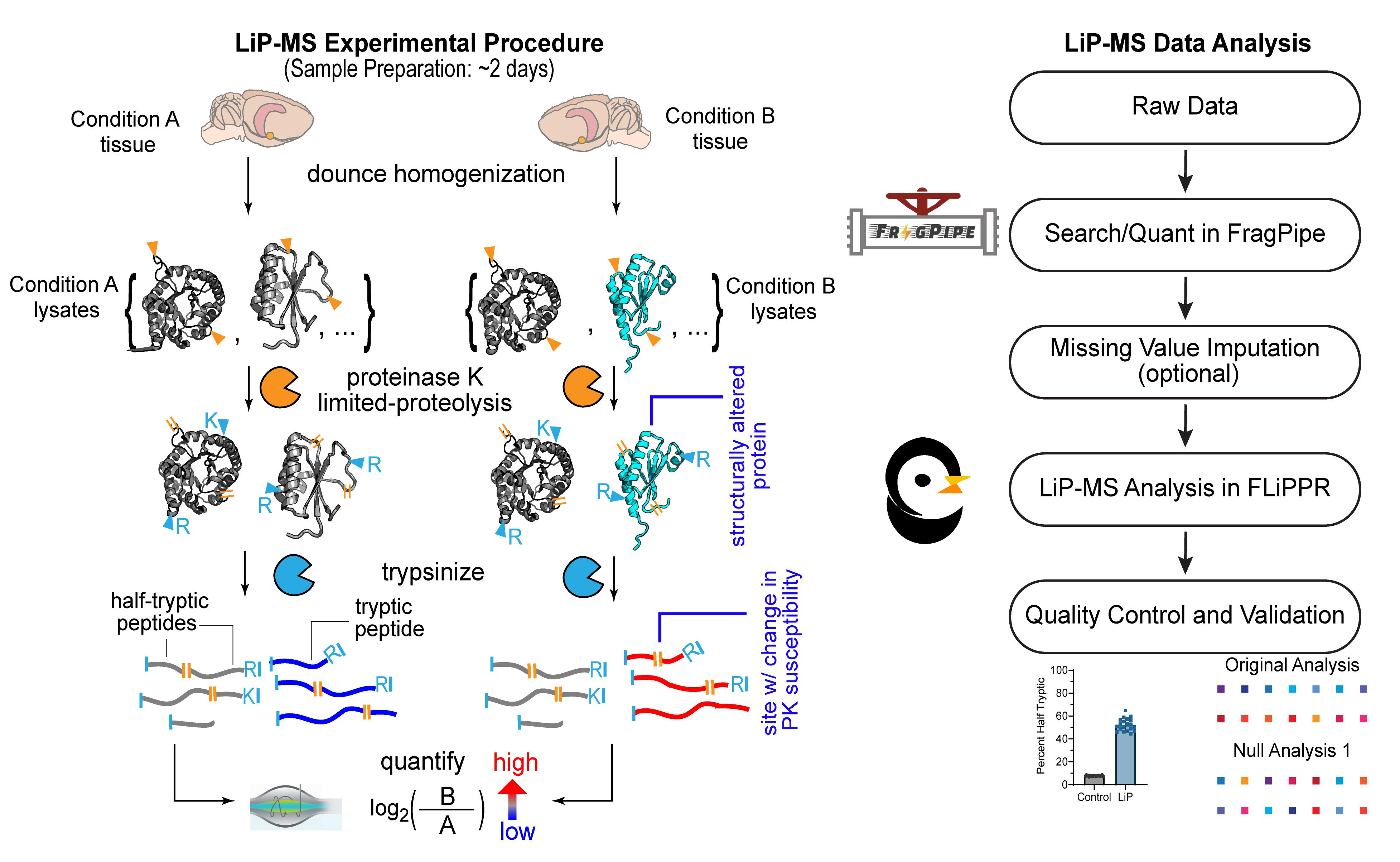
Limited proteolysis mass spectrometry (LiP-MS) experimental workflow and data analysis pipeline
Background
The study of protein structures is a cornerstone of molecular biology, as most proteins must be correctly folded to perform their cellular functions. However, many structural methods are low-throughput, studying one protein at a time [e.g., cryo-electron microscopy (cryo-EM), nuclear magnetic resonance (NMR), and x-ray crystallography]. In many systems, such as the environment of the aging brain, protein misfolding is known to occur, such as amyloid-β aggregation, seen in Alzheimer’s disease [1], or α-synuclein, seen in Parkinson’s disease [2]. However, such extreme misfolding events are uncommon, and only a few proteins are known to aggregate so dramatically. In an aging context, more subtle protein conformational changes have been demonstrated in multiple tissues [3–5]. Additionally, it is generally thought that the proteostasis network, which is responsible for ensuring that proteins are properly synthesized, correctly folded, and degraded when they become misfolded, declines with age [6–8]. Therefore, the conditions are present for potential widespread protein structural changes in a system such as the aged brain.
Limited proteolysis mass spectrometry (LiP-MS) is a technique to detect protein structural changes proteome-wide, with one modern incarnation developed by the Picotti group [9,10]. In LiP-MS, protein lysates undergo pulse proteolysis using proteinase K (PK), a protease that cleaves preferentially at solvent-exposed/flexible areas. This encodes structural information: if a protein is in a different conformation under a different condition, PK will cut at different places in the protein. Proteins then undergo complete digestion with trypsin, which cuts after arginine and lysine residues, and the resultant peptides are quantified using mass spectrometry. Differential cleavage by PK results in different peptide abundances between the two conditions, which can then be used to determine which proteins have different structures between the two conditions. Structural changes that can be detected by LiP-MS include conformational changes, differences in soluble oligomerization state, different binding to other proteins/ligands, etc. LiP does not reveal the exact nature of the structural change compared to a high-resolution method such as cryo-EM, but it has the advantage of being a proteome-wide technique. LiP-MS has already been used in a variety of contexts, such as to find protein structural changes in cerebrospinal fluid (CSF) between young and old mice [11], between young and old yeast extracts [12], between native bacterial lysates and refolded bacterial lysates [13], and between CSF of healthy and Parkinson’s disease patients [14].
Analysis of LiP-MS data can be performed using the free tools FragPipe [15] and FragPipe Limited-Proteolysis Processor (FLiPPR) [16]. However, care must be taken to ensure that analysis is done appropriately and does not induce false positives, especially in highly variable systems like tissue from outbred animals or from patient cohorts. Here, we describe how to perform LiP experiments on fresh-frozen rat brain tissue, how to prepare the samples for liquid chromatography–mass spectrometry (LC-MS), and how to acquire the raw data. We then describe how to analyze the data, first using FragPipe to process the raw LC-MS-MS data, and then using FLiPPR to process the FragPipe outputs. We also describe how to impute for missing values if needed, how to perform permutation analyses to ensure false positives are not being induced by the data analysis and/or imputation parameters, and how to assess experimental quality.
Materials and reagents
Biological materials
1. Long Evans rats (Charles River, catalog number: Crl:LE) or fresh-frozen brain tissue
Reagents
1. E-64 (Thermo Scientific, catalog number: 78434)
2. Dimethyl sulfoxide (DMSO) (Fisher Chemical, catalog number: D159-4)
3. Bestatin (Alfa Aesar, CAS number: 58970-76-6)
4. Phenylmethylsulfonyl fluoride (PMSF) (Acros Organics, CAS number: 329-98-6)
5. Deoxyribonuclease 1 (DNase) (Sigma-Aldrich, catalog number: DN25-1G)
6. Tris HCl (Millipore Sigma, catalog number: T15760)
7. Tris base (Millipore Sigma, catalog number: T1503)
8. Hydrochloric acid (HCl) (Sigma-Aldrich, CAS number: 7647-01-0)
9. Potassium chloride (KCl) (Sigma-Aldrich, catalog number: P3911)
10. Sodium chloride (NaCl) (Sigma-Aldrich, catalog number: S9888)
11. Magnesium chloride hexahydrate (MgCl2) (Fisher Chemical, catalog number: M33)
12. Glycerol (Fisher Chemical, catalog number: G33)
13. Proteinase K (PK) (Thermo Scientific, catalog number: 17916)
14. DL-dithiothreitol (DTT) (Sigma-Aldrich, catalog number: D0632)
15. Iodoacetamide (IAA) (Acros Organics, catalog number: 12227)
16. Ammonium bicarbonate (Thermo Scientific, catalog number: 393210050)
17. Ultrapure MS-grade water (Fisher Chemical, catalog number: W6-4)
18. MS-grade trifluoroacetic acid (TFA) (Fisher Chemical, catalog number: A116)
19. Ultrapure MS-grade acetonitrile (Fisher Chemical, catalog number: A955)
20. BCA Protein Assay kit (Thermo Scientific, catalog number: A55860)
21. Mineral oil (Thermo Scientific, catalog number: 415080025)
22. Urea, ultrapure, 99% (Thermo Scientific, catalog number: J65769.A4)
23. Trypsin, mass spectrometry grade (New England Biolabs, catalog number: P8101S)
24. Ultrapure MS-grade formic acid (Fisher Chemical, catalog number: A117-50)
Solutions
1. 100× E-64 Protease Inhibitor Stock (100× E-64) (see Recipes)
2. 100× Bestatin protease inhibitor stock (100× Bestatin) (see Recipes)
3. 100× Phenylmethylsulfonyl fluoride protease inhibitor stock (100× PMSF) (see Recipes)
4. 100× DNase stock (see Recipes)
5. 1 M Tris pH 8 Stock (see Recipes)
6. 1 M KCl stock (see Recipes)
7. 5 M NaCl stock (see Recipes)
8. 1 M MgCl2 stock (see Recipes)
9. Lysis buffer (see Recipes)
10. 20% glycerol solution (see Recipes)
11. PK stock (see Recipes)
12. DTT solution (see Recipes)
13. IAA solution (see Recipes)
14. Ammonium bicarbonate solution (AmBic solution) (see Recipes)
15. Buffer A (see Recipes)
16. Buffer B (see Recipes)
Recipes
1. 100× E-64
Prepare stocks of 1.5 mM E-64 in DMSO. Aliquot and store at -20 °C. Stocks can be thawed multiple times.
2. 100× Bestatin
Prepare stocks of 5 mM Bestatin in DMSO. Aliquot and store at -20 °C. Stocks can be thawed multiple times.
3. 100× PMSF
Prepare stocks of 50 mM PMSF in DMSO. Aliquot and store at -20 °C. Stocks can be thawed multiple times.
4. 100× DNase stock
Prepare a 10 mg/mL stock of DNase in Millipore water (MPW). Aliquot and store at -20 °C. Stocks can be thawed several times but should be kept on ice.
5. 1 M Tris pH 8 stock
| Reagent | Final concentration | Quantity or volume |
|---|---|---|
| Tris HCl | 88.8 g/L | 44.4 g |
| Tris base | 53 g/L | 26.5 g |
| MPW (to total volume) | n/a | 500 mL |
To approximately 400 mL of MPW, add 44.4 g of Tris acid and 26.5 g of Tris base. Adjust pH to 8 with HCl. Add MPW to a final volume of 500 mL. Autoclave to sterilize. Store at room temperature.
6. 1 M KCl stock
To approximately 400 mL of MPW, add 37.275 g of KCl and stir until dissolved. Add MPW to a final volume of 500 mL. Autoclave to sterilize. Store at room temperature.
7. 5 M NaCl stock
To approximately 400 mL of MPW, add 146.1 g of NaCl and stir until dissolved. Add MPW to a final volume of 500 mL. Autoclave to sterilize. Store at room temperature.
8. 1 M MgCl2 stock
To approximately 80 mL of MPW, add 20.33 g of magnesium chloride hexahydrate. Stir until dissolved, then add MPW to a final volume of 100 mL. Autoclave to sterilize. Store at room temperature.
9. Lysis buffer
| Reagent | Final concentration | Quantity or volume |
|---|---|---|
| 1 M Tris pH 8 stock | 20 mM | 1 mL |
| 1 M KCl stock | 150 mM | 7.5 mL |
| 5 M NaCl stock | 10 mM | 100 μL |
| 1 M MgCl2 stock | 2 mM | 100 μL |
| MPW | n/a | To 50 mL |
10. 20% glycerol solution
Prepare a 20% v/v solution of glycerol in MPW. Stir. Autoclave to sterilize.
11. PK stock
Measure an appropriate mass of PK and dissolve in a solution of 1:1 (v/v) 20% glycerol (Recipe 10; final glycerol concentration of 10%) and lysis buffer (Recipe 9) to a final PK concentration of 1 μg/μL. Aliquot into 1.5 mL tubes, flash freeze in liquid nitrogen, and store at -20 °C. Only thaw aliquots once.
12. DTT solution
Prepare a 700 mM DTT solution in MPW. The solution must be prepared fresh.
13. IAA solution
Prepare a 700 mM IAA solution in MPW. Protect from light. The solution must be prepared fresh.
14. AmBic solution
Prepare a 100 mM stock of ammonium bicarbonate (AmBic) in MPW. The solution must be prepared fresh.
15. Buffer A
| Reagent | Final concentration | Quantity or volume |
|---|---|---|
| Ultrapure MS-grade water | n/a | 200 mL |
| MS-grade TFA | 0.5% (v/v) | 1 mL |
Add TFA to the ultrapure water dropwise. Buffer A can be stored at room temperature for one week.
16. Buffer B
| Reagent | Final concentration | Quantity or volume |
|---|---|---|
| Ultrapure MS-grade water | 20% (v/v) | 20 mL |
| Ultrapure MS-grade acetonitrile | 80% (v/v) | 80 mL |
| MS-grade TFA | 0.5% (v/v) | 500 μL |
Add TFA to the ultrapure water and acetonitrile dropwise. Buffer B can be stored at room temperature for one week.
Laboratory supplies
1. 1.5 mL tubes (USA Scientific, catalog number: 1615-5500)
2. 2 mL tubes (Fisher Scientific, catalog number: 05-408-138)
3. C18 cartridges (Sep-Pak Vac 1cc) for desalting (Waters, catalog number: WAT054955)
4. 15 mL conical tubes (Sarstedt, catalog number: 62.554.100)
5. Mass spec vials (Thermo Scientific, catalog number: 6ERV11-03PPC)
6. Mass spec vial caps (Thermo Scientific, catalog number: 6ARC11ST1)
7. Disposable glass pipette (Fisher Scientific, catalog number: 13-678-20A)
8. 10 μL pipette tips (USA Scientific, catalog number: 1111-3700)
9. 200 μL pipette tips (USA Scientific, catalog number: 1111-0706)
10. 1,000 μL pipette tips (USA Scientific, catalog number: 1111-2721)
11. Gloves (Halyard, catalog number: 55082)
12. Kimtech Science Kimwipes (Kimberly-Clark Professional, catalog number: 34155)
Equipment
1. MilliQ water purification system (Millipore Sigma, model: EQ 7000)
2. Dounce homogenizer (Fisher Scientific, catalog number: 06-434)
3. Centrifuge (Eppendorf, model: 5430 R)
4. Temperature-controlled hot plate with stirring (IKA, model: C-MAG HS 7 control)
5. Glass container for oil bath (Pyrex, catalog number: 3140)
6. Metal grate for oil bath, taken from the bottom part of the water bath tube rack (United States Plastic Corp, catalog number: 96866)
7. Centrifuge (Eppendorf, model: 5425)
8. Vortex mixer (Benchmark, model: BenchMixer V2)
9. Shaking heat block (Benchmark, model: Multi-Therm)
10. Shaking heat block tube adaptor (Benchmark, model: H5000-15)
11. Analytical balance (Accuris Instruments, model: Series Dx)
12. Vacuum manifold (Zymo Research, catalog number: S7000)
13. Vacuum pump (Cole-Parmer, model: Air Admiral 79202-30)
14. Vacuum centrifuge (Eppendorf, model: Vacufuge plus)
15. -80 °C freezer (Thermo Scientific, model: Revco RLE series)
16. Centrifuge (Eppendorf, model: 5910 R)
17. Water bath sonicator (Rovsun, model: 230HT)
18. Microvolume UV-Vis spectrophotometer (Thermo Scientific, model: NanoDrop OneC)
19. UHPLC system (Thermo Scientific, model: UltiMate 3000)
20. Mass spectrometer (Thermo Scientific, model: Q Exactive HF-X)
21. Acclaim PepMap 100 Trap column, C18, 75 μm × 2 cm, 3 μm particle size (Thermo Scientific, catalog number: 164946)
22. Acclaim PepMap 100 Analytical Column, C18, 75 μm × 25 cm, 2 μm particle size (Thermo Scientific, catalog number: 164941)
23. Nanospray Flex ion source (Thermo Scientific, catalog number: ES071)
24. pH meter (Mettler Toledo, model: FiveEasy Plus FP20)
25. Pipettes (Eppendorf, catalog number: 2231300004)
26. 4 °C fridge (Fisher Scientific, catalog number: FBV05RPSA)
27. -20 °C freezer (VWR, catalog number: 10819-894)
Software and datasets
Note: All software is free to use.
1. FragPipe (https://fragpipe.nesvilab.org/, v23.1)
2. Anaconda Navigator (Anaconda Inc., v2.7.0)
3. VS Code (Microsoft, v1.105.1)
4. Missing value imputation script prefilter_impute_ion.ipynb (https://zenodo.org/records/15103402)
5. FLiPPR (https://github.com/FriedLabJHU/FragPipe-Limited-Proteolysis-Processor, v0.2.2)
6. Sample LiP data (https://www.ebi.ac.uk/pride/archive/projects/PXD052770)
Procedure
A. Lysis
1. Prechill lysis buffer and the Dounce homogenizer on ice. Remove 100× DNase stock from the freezer and thaw on ice. Remove 100× E-64, 100× Bestatin, and 100× PMSF from the freezer and thaw at room temperature.
2. For each sample, add 1 mL of lysis buffer to the prechilled Dounce homogenizer. Add 10 μL each of 100× DNase stock, 100× E-64, 100× Bestatin, and 100× PMSF to the Dounce homogenizer.
3. Obtain frozen brain tissue from the freezer and quickly add to the Dounce homogenizer.
Note: Approximately 0.1 g of tissue generally provides more than enough protein upon lysis for the experiment.
4. Dounce homogenize until sufficient lysis is achieved.
Note: Fifty strokes should be appropriate. It is unnecessary to completely remove the pestle from the lysate for each stroke.
Critical: The LiP samples should always be lysed fresh, and in a native-like buffer. Using frozen lysate is not appropriate, as a freeze-thaw may change protein structures and confound LiP. Do not use detergents in lysis buffers.
5. Remove the lysate from the Dounce homogenizer and transfer to a 1.5 mL tube. Keep on ice. Rinse the Dounce homogenizer well with MPW between each sample. Lyse all samples.
6. Centrifuge all lysates at 15,000× g for 15 min at 4 °C to clarify.
7. Carefully remove the supernatant to a new 1.5 mL tube. Discard the pellet. Keep samples at room temperature.
8. Determine the concentration of each sample using a BCA assay kit, according to the manufacturer’s instructions.
9. Normalize all samples to 1 μg/μL with lysis buffer.
B. Limited proteolysis (LiP)
1. Heat mineral oil bath to 105 °C. Remove PK stock from the freezer and keep on ice.
Critical: Do not proceed to the limited proteolysis step (step B3) until at least 2.5 h have passed since the addition of PMSF. PMSF is an irreversible serine protease inhibitor and will inhibit PK. However, after 2.5 h, sufficient hydrolysis of PMSF has occurred at pH 8 such that it is acceptable to add PK. (Note that this hydrolysis time is pH-sensitive and would need to be lengthened if the lysis buffer has a lower pH.) Additionally, keeping the samples at room temperature after clarification is important, as this increases the rate of PMSF hydrolysis (compared to the samples being left on ice), and proteins are stable due to the presence of the protease inhibitors.
2. From each sample, pipette 200 μL into a new 1.5 mL tube. This will be the tryptic control sample (trypsin only). Control samples are used to normalize for protein abundance differences between sample conditions and to ensure experimental quality.
3. For each LiP sample, pipette 2 μL of 1 μg/μL PK stock into a new 1.5 mL tube. Add 200 μL of sample into the tube and mix by pipetting. Incubate at room temperature for exactly 1 min from addition.
Note: A PK:lysate of 1:100 and 1 min minute incubation have been used for various sample types [13,17], but the ratio and incubation time may need to be empirically optimized if desired half-trypticity is not achieved (see Troubleshooting), especially for new sample types.
4. Place the LiP sample in an oil bath to quench the proteolysis reaction. Also, place the tryptic sample in the oil bath. Incubate for 5 min.
Critical: The LiP sample should be placed in the oil bath exactly 1 min from the addition of the sample to the PK. It is extremely important that this step is consistent between samples; otherwise, changes in proteolysis could occur from differing PK incubation times, as opposed to reporting on protein structural changes.
Note: We recommend using an oil bath, as opposed to a water bath, as water will boil and hot steam poses a safety issue when adding and removing samples from the bath.
5. Remove samples from the oil bath. Clean the exterior of the tube with a Kimwipe (or paper towel) and quickly spin down the samples to collect liquids to the bottom of the tube. Transfer each sample to a 2 mL tube containing 152 mg of urea, for a final volume of 314 μL and a final concentration of 8 M urea. Vortex to ensure complete dissolution.
Note: Aggregation may occur during the oil bath step. This is acceptable, as structural information is encoded before the heat quench. However, it is important to pipette up and down to resolubilize any aggregates to prevent sample loss. Also note that other protocols call for using deoxycholate to denature proteins [10]. We have found that detergents, even in trace amounts following their ostensible removal, can interfere with ionization during mass spectrometry, and have found better results with chaotrope-based denaturants.
C. Preparation of samples for mass spec
1. To each sample, add 4.5 μL of DTT solution (700 mM stock concentration) to a final concentration of 10 mM DTT. Incubate for 30 min at 37 °C in a shaking heat block, with shaking at 700 rpm.
2. To each sample, add 18 μL of IAA solution (700 mM stock concentration) to a final concentration of 40 mM IAA. Incubate for 45 min at room temperature in the dark.
Note: IAA is light-sensitive, and it is best to minimize exposure of the samples to light during this step.
3. To each sample, add 1,010 μL of AmBic solution (100 mM stock concentration) to dilute the urea to a final concentration of 2 M.
4. Prepare mass spec–grade trypsin by dissolving trypsin in MPW to a final concentration of 1 μg/μL. Add 4 μg of trypsin per sample (final trypsin:protein ratio of 1:50) by adding 4 μL of the 1 μg/μL stock. Incubate the samples overnight at 25 °C in a shaking heat block, with shaking at 700 rpm.
Note: Trypsin should be incubated for a minimum of 12 h to ensure complete digestion. We do not trypsinize at 37 °C so as to minimize the decomposition of urea and attendant carbamylation that can occur at lysine residues.
5. Add mass spec–grade TFA to a final concentration of 1% by adding 16.6 μL of TFA to each sample.
Caution: TFA is a strong acid and should be handled in a fume hood and with proper PPE.
Note: TFA addition produces carbon dioxide, which should be dissipated by pipetting up and down until bubble formation ceases.
6. To desalt samples, place C18 columns (Sep-Pak) on a vacuum manifold. Condition each column by adding 1 mL of buffer B (see Recipes). Turn on the vacuum, open the tap, and allow the buffer to pass through the sorbent, closing the tap just before the buffer completely passes through. Repeat the conditioning step with an additional 1 mL of buffer B.
Note: Do not allow the sorbent to dry at any point during the desalting procedure.
7. Equilibrate each cartridge by adding 1 mL of buffer A (see Recipes) and allowing it to pass through as above. Repeat three additional times.
8. Add the sample to the cartridge and allow it to pass through the sorbent.
Note: To allow as much binding as possible to the sorbent, consider lowering the vacuum pressure so the sample passes over the sorbent more slowly. For example, open several unused taps on the vacuum manifold.
9. Wash each cartridge with 1 mL of buffer A. Repeat three additional times.
10. Remove each cartridge from the vacuum manifold and place in a 15 mL conical tube. Place the conical tubes into the centrifuge and spin at 20× g for 5 min. This works best in a swing-bucket centrifuge such as the Eppendorf 5910 R.
Note: Once the sample has been added to the cartridge, do not add buffer B until the cartridge has been removed from the vacuum manifold. Otherwise, the sample will be lost.
11. Transfer eluate from the 15 mL conical tube to a 1.5 mL centrifuge tube. Place the tube in a vacuum centrifuge until the sample is completely dried down. Store samples at -80 °C. Perform vacuum centrifugation without elevated temperature.
Note: A small tan/light brown pellet may be visible; these are the dried-down peptides. The peptide pellet is not always visible.
Pause point: Samples can be stored at -80 °C for several months until they are ready to be shot on the mass spectrometer.
12. To resuspend samples, add 200 μL of 0.1% LC/MS-grade formic acid in ultrapure MS-grade water. Pipette up and down several times until the peptide pellet is no longer visible.
Note: Do not directly touch the pellet with a pipette tip, as the peptide pellet can stick to the tip, and sample loss could occur.
13. Sonicate samples in a water bath sonicator for 5 min to dissolve peptides. Vortex each sample and quickly spin down in a benchtop centrifuge.
14. Measure the concentration of the peptides using a microvolume UV-Vis spectrophotometer at a wavelength of 280 nm. Blank the spectrophotometer with the 0.1% formic acid solution.
Note: If the absorbance at 280 nm is much greater than 1 (absorbance of 1 is approximately 1 mg/mL), dilute the sample with additional 0.1% formic acid until an absorbance reading of <1 is achieved.
15. Transfer 50 μL of sample to a mass spec vial compatible with the mass spectrometer that will be used.
Critical: There can be no particulate in the mass spec vial. If any particulate is present, spin down the sample in a benchtop centrifuge, remove the sample from the top, and add that to the vial. Also, ensure there are no air bubbles in the sample vial.
Note: Extra sample remaining after transferring to the mass spec vial can be vacuum-centrifuged to dryness and stored at -80 °C.
D. Mass spec acquisition
Note: Acquisition can be carried out either using data-dependent acquisition (DDA) or data-independent acquisition (DIA). The analysis will differ slightly depending on the acquisition method.
1. Place a mass spec sample vial in the autosampler and inject 0.5–1 μg of sample onto the UHPLC-MS system. Keep the amount injected consistent between all samples in the study. It is best to inject a small volume (for example, 1 μL), but larger volumes can be injected if the sample is too diluted. Mobile phase A is 0.1% formic acid in ultrapure MS-grade water, and mobile phase B is 0.1% formic acid in ultrapure MS-grade acetonitrile.
2. For each injection, allow peptides to accumulate on the trap column for 10 min at 2% mobile phase B. Then, switch the trap column to be in line with the separating column.
3. Separate peptides on the separating column. Flow rate is kept constant at 0.3 μL/min. A typical separating method with a length of 150 min (Table 1) is appropriate for DDA. For DIA, a shorter 85-min method (Table 2) may be reasonable, but empirical testing to determine appropriate gradient length is advisable. Gradient methods may need to be empirically optimized. Note that percent B increases linearly in steps where a change in percent B occurs over time. Ensure that 0.1% formic acid in ultrapure MS-grade water blanks are run between every 4–6 samples.
Table 1. Example 150-min gradient method
| Minutes | Percent B |
|---|---|
| 0–10 | 2% |
| 10–15 | 2%–5% |
| 15–110 | 5%–25% |
| 110–135 | 25%–40% |
| 135–140 | 40% |
| 140–145 | 90% |
| 145–146* | 90%–2% |
| 146–147 | 2%–90% |
| 147–148 | 90%–2% |
| 148–149 | 2%–90% |
| 149–150 | 90%–2% |
* This step onward represents a sawtooth gradient to eliminate residual peptides from the column
Table 2. Example 85-min gradient method
| Minutes | Percent B |
|---|---|
| 0–10 | 2% |
| 10–15 | 2%–5% |
| 15–62 | 5%–25% |
| 62–75 | 25%–40% |
| 75–80 | 40%–90% |
| 80–81* | 90%–2% |
| 81–82 | 2%–90% |
| 82–83 | 90%–2% |
| 83–84 | 2%–90% |
| 84–85 | 90%–2% |
* This step onward represents a sawtooth gradient to eliminate residual peptides from the column
4. Ionize peptides using a nanospray source. Collect mass spectra using the following settings for DDA (Table 3) or DIA (Table 4). Spectra are collected in positive ion mode.
Table 3. Data-dependent acquisition (DDA) mass spec settings. Example parameters for data-dependent acquisition settings.
| Setting | Value |
|---|---|
| Scan range | 350–1,500 m/z |
| Number of data-dependent scans per full MS scan | 20 |
| Resolution (full scan) | 120,000 |
| AGC target (full scan) | 3 × 10⁶ |
| Maximum injection time (full scan) | 64 ms |
| HCD collision energy | 27% |
| Resolution (data-dependent scan) | 15,000 |
| AGC target (data-dependent scan) | 1 × 10⁵ |
| Minimum AGC target (data-dependent scan) | 8 × 10³ |
| Maximum ion injection time (data-dependent scan) | 55 ms |
| Isolation window | 1.4 m/z |
Table 4. Data-independent acquisition (DIA) mass spec settings. Example parameters for data-independent acquisition settings.
| Setting | Value |
|---|---|
| Scan range | 350–1200 m/z |
| Resolution (full scan) | 120,000 |
| AGC target (full scan) | 3 × 10⁶ |
| Maximum injection time (full scan) | 64 ms |
| HCD collision energy | 28% |
| Resolution (data-independent scan) | 30,000 |
| AGC target (data-independent scan) | 1 × 10⁵ |
| Maximum ion injection time (data-independent scan) | 50 ms |
| Isolation window | 16 m/z |
Note: Optimal HCD collision energies can vary somewhat from instrument to instrument, even of the same nominal type. Also note that these experiments were conducted on Q Exactive HF-X. DIA with narrower isolation windows is likely to improve coverage on a faster frontier instrument such as an Astral or Astral Zoom. DIA settings were determined empirically, but several considerations regarding DIA method development can be found in the literature [18,19].
Data analysis
A. Search and label-free quantification (LFQ) using FragPipe
Note: FragPipe is a free application developed by the Nesvizhskii lab. It utilizes MSFragger for database search [15], IonQuant for LFQ analysis for DDA data [20], and DIA-NN for DIA data [21]. Tutorials for the use of FragPipe can be found on https://fragpipe.nesvilab.org/, including instructions on how to download and set up FragPipe.
A1. DDA data
1. Open FragPipe. In the Workflow tab, press Add files to add raw data files. Run two separate analyses: one with all of the trypsin-only control samples, and one with all of the LiP samples. Label samples of the same condition with the same experiment name (for example, “wild-type”) and label the bioreplicates as unique increasing integers within that condition. Repeat for the other conditions.
2. Still in the Workflow tab, select the LFQ-MBR workflow. All settings are default, with the following exceptions (Table 5). Settings can be optimized. It is best practice to run semi-specific searches (cleavage setting set to SEMI) on both the control and LiP analyses for quality control purposes.
Table 5. Non-default LFQ-MBR FragPipe settings. Parameters in FragPipe for data-dependent acquisition settings. Settings not mentioned in this table are the default in FragPipe. “Setting location” refers to the tab where the setting is found.
| Setting location | Setting | Value |
|---|---|---|
| MSFragger | Precursor mass tolerance | -10 to 10 ppm |
| MSFragger | Cleavage | SEMI |
| MSFragger | Output format | TSV_PEPXML_PIN |
| Quant (MS1) | MBR ion FDR | 0.05 |
| Quant (MS1) | MBR top runs | 100 |
3. In the Database tab, for the FASTA file path, either select Download and select the species of your sample, or select Browse and upload a FASTA file of the proteome (for example, from UniProt, https://www.uniprot.org). If there are no decoys in the file (indicated below the file path), click add decoys. Decoys and contaminants can also be added when downloading the proteome through FragPipe. The FASTA should comprise 50% decoys.
4. In the Run tab, select an output directory for the results file. It is helpful to create a new folder. Click RUN to start the analysis.
A2. DIA data
1. Open FragPipe. In the Workflow tab, press Add files to add raw data files. Run two separate analyses: one with all of the trypsin-only control samples, and one with all of the LiP samples. Label samples of the same condition with the same experiment name (for example, “wild-type”) and label the bioreplicates as unique increasing integers within that condition. Repeat for the other conditions.
2. Still in the Workflow tab, select the DIA_SpecLib_Quant workflow. All settings are default, with the following exceptions (Table 6). Settings can be optimized. It is best practice to run semi-specific searches (cleavage setting set to SEMI) on both the control and LiP analyses for quality control purposes.
Table 6. Non-default DIA_SpecLib_Quant FragPipe settings. Parameters in FragPipe for data-independent acquisition settings. Settings not mentioned in this table are the default in FragPipe. “Setting location” refers to the tab where the setting is found.
| Setting location | Setting | Value |
|---|---|---|
| MSFragger | Precursor mass tolerance | -10 to 10 ppm |
| MSFragger | Cleavage | SEMI |
| MSFragger | Output format | TSV_PEPXML_PIN |
| Quant (DIA) | FDR | 0.05 |
3. In the Database tab, for the FASTA file path, either select Download and select the species of your sample or select Browse and upload a FASTA file of the proteome (for example, from UniProt, https://www.uniprot.org). If there are no decoys in the file (indicated below the file path), click add decoys. Decoys and contaminants can also be added when downloading the proteome through FragPipe. The FASTA should comprise of 50% decoys.
4. In the Run tab, select an output directory for the results file. It is helpful to create a new folder. Click RUN to start the analysis.
B. (Optional) Imputation of missing values
Note: DDA data generally have more missing values than DIA data. Missing value imputation is optional, depending on how strict a cutoff is desired, for example. Any imputation method should be evaluated to ensure it is not creating false positives (see Data analysis, section D). Imputation also may not be necessary if using samples with less intra-group variability, such as replicate cultures of microorganisms.
B1. DDA data
1. Download the missing value imputation script (prefilter_impute_ion.ipynb) from Zenodo (https://zenodo.org/records/15103402).
2. Open Anaconda Navigator and launch VS Code. Open prefilter_impute_ion.ipynb.
3. Change the “fragpipe_output_path” variable to point to the folder containing the folders with the FragPipe outputs.
4. Change the “lip_ion_tsv” variable to point to the combined_ion.tsv file in the appropriate FragPipe output folder.
5. Change the “ctrl_name” and “test_name” variables to the names of the two conditions that will be compared in the future. Ensure that the name is the same as the label entered for the “experiment” when running the original FragPipe job.
6. Set the values of “n_reps_ctrl” and “n_reps_test” to the number of replicates for the condition indicated above in “ctrl_name” and “test_name”, respectively.
7. Next, decide imputation conditions. In addition to DDA generally having more missing values, LiP can also contribute to additional missing values, since PK cuts are somewhat stochastic, and even a true structural change may not manifest as a PK cut at the exact same location in every single sample. Therefore, imputation is most appropriate when one condition has very few missing values, and the other condition is completely or mostly missing. There are two main parameters to consider when deciding when missing values should be imputed: the maximum number of missing values in an ion feature where imputation is acceptable, and the exact number of missing/present values to trigger imputation.
8. First, decide the maximum number of missing values within a condition where imputation is still acceptable. For example, if there are 6 replicates in each condition, one may choose to only consider ion features for imputation when there are a maximum of two missing values for each condition. This parameter may need to be determined empirically (see section D).
Note: It is best to have a similar threshold on a percentage basis for both conditions. For example, it would not be appropriate for one condition with 10 samples to accept only 2 max missing values, but the other condition with 8 samples to accept 5 max missing values.
9. Set “n_max_missing_ctrl” and “n_max_missing_test” to the maximum number of missing values in the control and test conditions, respectively, that are allowed before an ion feature is filtered out.
10. Decide imputation conditions. For example, one may choose to impute for a particular ion when one condition has greater than two-thirds of the samples with values, but the other condition for that same ion is missing values in more than half of the samples. This parameter may also need to be determined empirically.
11. In prefilter_impute_ion.ipynb, change the values in the following function to match the decided-upon imputation conditions. For example, here, if the control condition has more than four missing values and the test condition has fewer than or equal to four missing values in that same ion, imputation will occur. Additionally, if the control condition has fewer than or equal to three missing values while the test condition has more than six missing values, imputation will occur.
imp_df = lip_ion_df.with_columns(# Count the number of zeros intensity replicates pl.concat_list(lip_ctrl_var_cols["Intensity"]).list.count_matches(0).alias(f"{ctrl_name} ZC"), pl.concat_list(lip_test_var_cols["Intensity"]).list.count_matches(0).alias(f"{test_name} ZC"),).filter( ((pl.col(f"{ctrl_name} ZC") > (4)) & (pl.col(f"{test_name} ZC") <= (4))) |((pl.col(f"{ctrl_name} ZC") <= (3)) & (pl.col(f"{test_name} ZC") > (6))))12. Immediately below, the imputation occurs. Here, missing values are replaced with an imputed value in the condition that is missing more data (for example, imputation occurs above when the test condition is missing more than six values and the control condition is missing less than or equal to three values. Missing values are not imputed in the control condition in this case, only in the test condition). The imputed value is determined using the function np.random.normal. The default imputation is to select a random number from a Gaussian distribution with a mean of 1 × 10⁴ and a standard deviation of 1 × 10³. These parameters can be changed if desired. Also, ensure the zero count filters match the filters in Data analysis, step B1.11 (this occurs twice).
13. In the final code block, ensure that the zero count filters again match the filters in Data analysis, step B1.11.
14. Run prefilter_impute_ion.ipynb. This generates a tsv called “imp_combined_ion.tsv,” which contains the data from the original combined_ion.tsv generated by FragPipe, except also containing imputed values.
B2. DIA data
1. Missing value imputation should not be necessary for DIA data.
C. Running FLiPPR
Note: FLiPPR was developed by Edgar Manriquez-Sandoval in the Fried lab. The algorithm of FLiPPR is described in detail elsewhere [16]. Install FLiPPR using the command python -m pip install flippr.
C1. DDA
1. In a Jupyter notebook, import FLiPPR.
import flipprfrom flippr import Study2. Create a study, indicating the locations of the FragPipe output folder for the analysis of the LiP samples and the analysis of the trypsin-only control samples. Indicate that the acquisition type is DDA. Correct import can be checked by calling “study.samples” and the experimental conditions as entered into FragPipe should be shown.
study = flippr.Study(lip = "path/to/fp/lip/output", trp="path/to/fp/control/output", method="dda")study.samples3. Create an experimental process. Give the process a name, indicate the experimental conditions to be compared, and indicate the number of replicates. Note that the “test” condition is the numerator of generated ratios, while the “control” condition is the denominator. Here, x is the number of replicates of the control condition, and y is the number of replicates of the test condition. If a trypsin-only control is used for normalization, this will also be indicated here. Ensure that the _ctrl and _test parameters have the same name as the experimental condition used in FragPipe.
study.add_process(pid="process", lip_ctrl="wildtype", lip_test="conditionA", n_rep=(x,y), trp_ctrl="wildtype", trp_test="conditionA", trp_n_rep=(x,y))Note: The trypsin-only control samples are used to normalize the LiP values if there is a significant difference in protein abundance between the two conditions, as otherwise a difference in peptide abundance in the LiP sample could be misinterpreted as indicative of a structural change. Ensure that the trypsin-only control samples correspond to the same conditions that are compared in the LiP experiment. Also note that some procedures use the trypsin-only samples to normalize at the peptide level [22]. We have not implemented this practice here because it requires discarding the half-tryptic peptides, which contain high-resolution structural information.
4. Parameters can be changed within FLiPPR from their defaults using rcParams. For example, the maximum number of missing intensities to accept without filtering out the ion feature can be modified from the default of 1. Note that currently, this number applies to both conditions, even if there is a different number of replicates. In the case of a desire for custom filtering based on missing values, this should be done to the combined_ion.tsv file, for example, during the imputation step.
flippr.rcParams["ion.missing_intensity_thresh"] = 35. Next, run the study with the following command:
results = study.run()Note: If using an alternative combined_ion input (such as a file with imputed values as generated in Data Analysis, Section B), create a new folder for the FragPipe output, containing the modified combined_ion.tsv with the imputed values, ensuring it is named combined_ion.tsv. The new folder must, at minimum, contain combined_ion.tsv, combined_protein.tsv, and experiment_annotation.tsv. Ensure that a folder with the original FragPipe outputs is retained.
6. Results can be written to Excel.
results_process = results[“process”]summaryProcess= results_process.protein_summarysummaryProcess.write_excel("ProteinSummaryProcess.xlsx", freeze_panes=(1,0))peptideProcess= results_process.peptidepeptideProcess.write_excel("PeptideSummaryProcess.xlsx", freeze_panes=(1,0))control = results_process.trp_proteincontrol.write_excel('ControlProcess.xlsx', freeze_panes=(1,0))a. The protein_summary file contains protein accessions, along with the number of significant peptides. A peptide is considered significant if there is a two-fold change in abundance of the peptide and a Benjamini–Hochberg (BH) multiple-hypothesis corrected false discovery rate (FDR) adjusted p-value of less than 0.05.
Note: It is best to reference the columns that use adjusted p-values, as multiple hypothesis correction plays an important role in adjusting for coverage bias, which results in type I statistical errors.
b. The peptide file, among other information, lists each peptide and the accession number of the protein it is from, the location of the peptide, whether it is fully tryptic or half-tryptic, and the fold change and adjusted p-value. A peptide can be considered significantly different if the log2-normalized fold change (“Log2 Normalized FC” column) is greater than one (two-fold change) and the -log10 adjusted p-value (“-Log10 Adj. P-value” column) is greater than 1.301 (adjusted p-value of less than 0.05).
c. The trp_protein file outputs proteins and contains the fold-change and p-value for the trypsin-only samples. This file can be helpful for seeing if there are any proteins that have significantly different abundances between the two conditions. Proteins with greater than 2-fold abundance differences with a p-value of less than 0.01 are considered significantly different, and the abundance of peptides from those proteins in the LiP data is corrected within FLiPPR. These thresholds can be changed using flippr.rcParams. We generally use non-adjusted p-values from the trypsin-only control study to assess the need for normalization.
7. A protein can be considered a LiP hit if it has two or more peptides detected (“No. of Valid Peptides” column in the protein_summary file), and of those, two or more are considered significant [“No. of Significant Peptides (Adj. P-value)” column in the protein_summary file]. Proteins with two or more peptides detected, with one or zero significant peptides, can be considered non-hits, meaning there is likely no structural difference between the two conditions. Proteins with one peptide only do not have enough information to be categorized either way. A hit means that, based on the differential cleavage locations of PK, the protein likely has a different structure between the two conditions tested. A structural difference could be a conformational change, a difference in oligomerization state, a bound vs. an unbound state, etc.
C2. DIA
1. Run FLiPPR as above, with the following changes. First, in the study, the method should be indicated as DIA.
study = flippr.Study(lip = "path/to/fp/lip/output", trp="path/to/fp/control/output", method="dia")study.samples2. If there is any imputation/prefiltering being done, the file to edit is report.pr_matrix.tsv (as opposed to combined_ion.tsv, as in DDA), which can be found in the dia-quant-output folder generated in the output folder from FragPipe. Again, always retain a folder of original FragPipe outputs. The new folder with prefiltering/imputed values should minimally contain ion.tsv, experiment_annotation.tsv, and a folder called “dia-quant-output” containing report.pr_matrix.tsv and report.pg_matrix.tsv. Additionally, there are generally fewer missing data in DIA experiments compared to DDA experiments, so imputation is generally unnecessary, at least within our experience.
D. Quality control and validation
1. Several metrics can be used to determine the quality of the limited proteolysis steps and the mass spec acquisition (Figure 1).
a. Count the number of identified proteins (Figure 1A). If one sample has many more or many fewer proteins than the rest of the samples, this can indicate a quality issue. Proteins can be counted in the protein_summary file output from FLiPPR. Alternatively, proteins can be counted after FragPipe. For DIA analyses, one can use the report.stats.tsv file generated in the dia-quant-output folder, whereas for DDA analyses, the protein.tsv files generated for each sample (located in the folders with the sample names) can be used. A filter of a ProteinProphet score of >0.95 can be used to avoid including low-quality matches in these counts, if desired.
b. Similarly, count the number of identified peptides (Figure 1B). Peptides can be counted in the peptide file output from FLiPPR. Alternatively, peptides can be counted after FragPipe. For DIA analyses, one can use the number of precursors in the report.stats.tsv file generated in the dia-quant-output folder, whereas for DDA analyses, the peptide.tsv files generated for each sample (located in the folders with the sample names) can be used. A filter of a PeptideProphet score of >0.95 can be used, if desired.
c. Determine the percent half-trypticity of the peptides (Figure 1C). Fully tryptic peptides are peptides where both the N-termini and the C-termini were cut by trypsin, meaning the last amino acid of the peptide is arginine or lysine, and the amino acid preceding the first amino acid (known from the FASTA) is arginine or lysine. For a half-tryptic peptide, either the N- or C-terminus was cut by trypsin, but not both. The FLiPPR peptide file output lists if a peptide is fully tryptic or half-tryptic in the “Cleavage Type” column, where FULL_TRP indicates a fully tryptic peptide and N_SEMI and C_SEMI indicate a half-tryptic peptide. Alternatively, the FragPipe-generated peptide.tsv files can be used for DDA analyses, with the advantage of being able to calculate half-trypticity of each individual sample.
Note: Half-trypticity should be relatively low for the control (less than 20%) and relatively high for the LiP samples (approximately 50%). High half-trypticity in the control suggests that endogenous proteases or other sources are leading to protein degradation; in this case, it will be unclear whether peptides were cut by PK or some other source, confounding analysis. Low half-trypticity in the LiP samples may lead to insufficient structural information upon analysis. See Troubleshooting for more information.
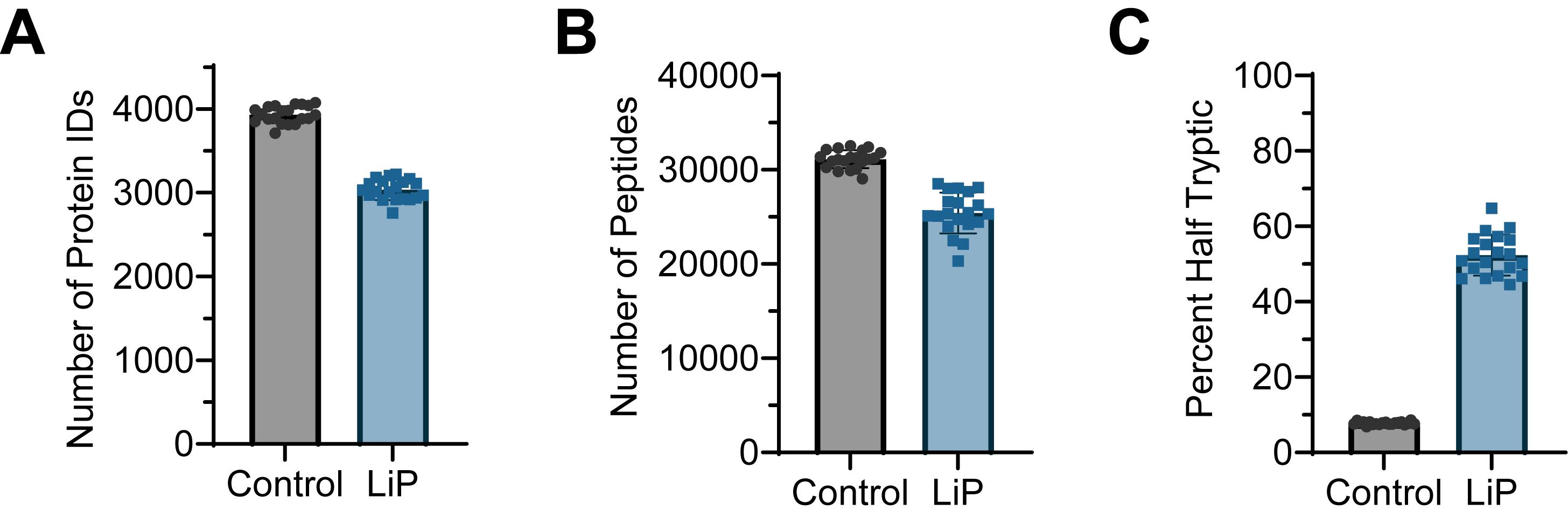
Figure 1. LiP and acquisition quality control metrics. (A) Number of proteins identified in the trypsin-only control and PK-containing LiP samples from the sample LiP data (see Software and datasets). Each point represents the number of proteins from individual protein.tsv files. Proteins must have a ProteinProphet score greater than 0.95 to be counted. (B) Number of peptides identified in the control and LiP samples from the sample LiP data. Each point represents the number of peptides from individual peptide.tsv files. Proteins must have a PeptideProphet score of greater than 0.95 to be counted. (C) Each point represents, per sample, the percent of peptides that are half-tryptic, meaning one side of the peptide was cut by PK and the other by trypsin.
2. LiP experiments, especially those performed with outbred animals or patient samples, may have high intra-group variation between samples. Therefore, false discovery rate (FDR) should be tested empirically to ensure that LiP hits are indicative of real and robust structural changes between conditions, and not due to high sample variation. One way to achieve this is by performing a permutation analysis (also referred to as a null analysis), where the samples are (incorrectly) randomly assigned to the two condition labels, and the analysis is run as normal. If the data analysis pipeline (including any imputation, filtering, etc.) is robust, there should be few or (ideally) zero hits in the permutation analysis. The number of hits of null analyses can be reported to quantify the confidence of a dataset and to estimate true FDR.
a. Generate the null analyses (Figure 2). Use a random number generator to randomize labels. Ensure they are reasonably distributed (a null analysis with only one replicate “incorrectly” categorized will not be meaningful). For example, if there are 7 replicates of condition A and 6 replicates of condition B, a null analysis could have one condition “A” that includes 3 replicates from original condition A and 4 replicates from original condition B. Multiple null analyses (for example, three different analyses) should be performed for a more accurate empirical FDR estimation.
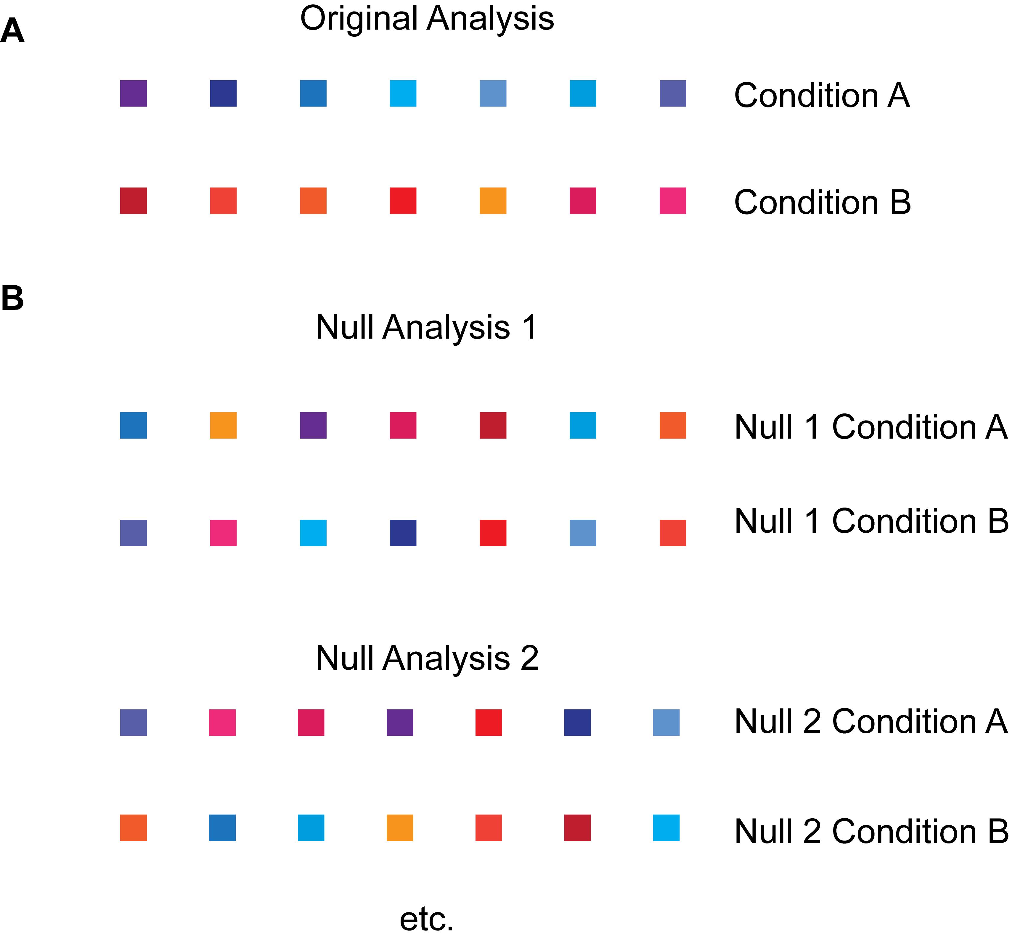
Figure 2. Creating appropriate null analyses. (A) In the original analysis, which represents the actual experimental conditions, the samples from condition A are represented by blue/purple boxes. Samples from condition B are represented by red/orange boxes. (B) Two example null analyses are shown. Samples from the original analysis were assigned random labels to create example null analyses. The null analyses contain samples from both real conditions in each null condition.
b. For each null analysis, process the data in the same manner as the original analysis. Starting from FragPipe, run a new LFQ with the original raw files, changing the labels according to the null analysis scheme. Next, run FLiPPR using the new FragPipe outputs. Determine the number of hits from the protein_summary output from FLiPPR. If the original analysis is robust, there should be many fewer hits in the null analyses compared to the original analysis. The average number of hits from the null analyses can be divided by the number of hits in the original analysis to generate an estimated empirical FDR. With only a few null analyses, this is not an extremely accurate measure, but it can serve as a helpful estimation.
c. If the null analysis shows a high percentage of false positive hits compared to the number of hits in the original analysis, there are several potential actions to take. First, if imputation is being used, it is possible that the imputation is confounding the analysis. Edit the imputation conditions (for example, under what conditions imputation occurs) and see if the ratio of hits from the original analysis to hits from the null analyses improves. It is also possible that the samples are too variable to get a very low FDR, or that there were not enough replicates used, in which case the null analyses can help assign an appropriate level of confidence to the hits in the original analysis. Our general experience has been that more false positives occur in null analyses of DDA-based datasets compared to DIA-based datasets.
E. Further investigation
1. Proteins with two or more significantly different peptides between the two conditions (in protein_summary file from FLiPPR) can be considered hits, where they have a different structure between the two different experimental conditions. These proteins can be further investigated individually with follow-up experiments. Additionally, analysis can be performed to determine what types of proteins in general are hits (for example, gene ontology analysis) or the characteristics of hit proteins (asking if they have a higher average molecular weight than non-hit proteins, for example).
2. Among hit proteins, the locations of the significantly different cuts can be determined from the peptide file output from FLiPPR. Half-tryptic peptides can resolve a structural difference to a single residue; tryptic peptides, on the other hand, have a resolution equal to the length of the peptide. If multiple significant cut sites localize on a protein, there can be some assessment as to the location of the structural change. However, alternative structural methods represent the best approach to critically test predictions from LiP-MS, especially on individual proteins.
Validation of protocol
Part of this protocol has been used and validated in the following research article:
• Tarbox et al. [17]. Proteins with cognition- associated structural changes in a rat model of aging exhibit reduced refolding capacity. Science Advances.
The reproducibility of the LiP protocol (using DDA acquisition) was investigated, and the results are shown in supplementary Figure S4 of [17]. Overall, this protocol is reproducible in terms of technical instrument variation (multiple injections of the same LiP sample are highly similar) and limited proteolysis variation (treatments of the same lysate with PK yield similar results).
Especially when using a highly variable system, such as outbred animals, it is important to have sufficient replicates. It is also important to use appropriate missing-value imputation, if used (see Data analysis, section B). Using null analyses to empirically ensure that the false discovery rate is appropriate can be extremely helpful for determining the trustworthiness of the LiP hits (see Data analysis, section D) and is strongly recommended.
Other researchers have confirmed that DIA is an acceptable acquisition method for LiP-MS [23].
General notes and troubleshooting
General notes
1. LiP-MS has the advantage of being a proteome-wide method, but it is not ideal for determining exact structural differences of individual proteins. Some proteins may only have a few significantly different peptides, and while their localization may be able to provide some structural insight, this is still a low-resolution method. As such, orthogonal structural methods can be helpful for investigating individual proteins or for corroborating proteome-wide LiP results. Additionally, LiP is not necessarily able to comprehensively capture all structural changes, as not all structural changes will lead to a difference in PK accessibility.
2. LiP-MS cannot differentiate between different types of structural changes. For example, if a protein has a different structure between two conditions, it may be that it is in a different conformation, or it is dimerizing in one condition, or binding another protein/ligand in one condition, etc.
3. LiP-MS is biased toward more abundant proteins, and structural changes in lower-abundance proteins can be challenging to detect.
4. LiP-MS can be applied to purified proteins and complexes, not just complex samples such as tissue homogenates.
5. LiP-MS can be applied to many cell types, including E. coli, yeast, other tissues, etc. Regardless of the original protein source, gentle lysis methods are essential. Dounce homogenization, used here, is appropriate, but would not work well on tougher tissues or cells with cell walls. In much of our work on microorganisms, we have lysed cells using cryo-milling [13]. A lysis method such as sonication is not advisable, as structural changes may be induced by the lysis method itself. Detergents are also problematic because they can unfold (or partially unfold) proteins.
6. LiP-MS only reports on structural changes between soluble proteins, as aggregates and membrane proteins are removed during the clarification of the detergent-free extract.
Troubleshooting
Problem 1: High percentage of half-tryptic peptides in the control samples.
Possible cause: Insufficient native protease inhibition.
Solutions: Ensure that tissue quality is sufficient (for example, that it was flash-frozen quickly during collection). Ensure protease inhibitor stocks are fresh. Make sure lysis is performed on ice, and the lysis buffer is prechilled. If the issue persists, consider optimizing which protease inhibitors are used and/or the amount used.
Problem 2: Low percentage of half-tryptic peptides in the LiP samples.
Possible causes: Under-digestion or over-digestion of samples. Too many cuts by PK will create peptides where both N- and C- termini were cut by PK, which will not be detected in a semi-specific search.
Solutions: Optimize the PK digestion step by either increasing or decreasing the time of PK digestion before the oil bath quench, or by increasing or decreasing the ratio of PK to sample protein. Ensure adequate time has elapsed between PMSF addition and PK addition.
Problem 3: High false discovery rate after null analyses.
Possible causes: Too few replicates, inappropriate imputation conditions, or no detectable protein structural differences between the sample conditions.
Solutions: Perform more sample replicates and optimize imputation conditions. If there are no detectable protein structural differences between the two conditions, it is possible that the difference between the conditions is not sufficient to induce protein structural changes, and different experimental conditions should be used. LiP is not an extremely sensitive method, since it is proteome-wide, so subtle structural changes between conditions may not be detected.
Problem 4: Low peptide identification numbers/intensities.
Possible causes: Inappropriate acquisition method parameters or LC/MS maintenance issues.
Solutions: Ensure that the acquisition method is appropriate, especially for DIA-based acquisition methods where the isolation window design is important (see [18,19] for considerations concerning DIA acquisition method design). Acquisition methods may need to be optimized empirically, especially since optimal collision energies can vary between instruments. Alternatively, ensure that the mass spectrometer is properly calibrated and the source is clean, as these issues can cause low intensity. Confirm appropriate peak shapes and verify proper performance of the LC (no fronting/tailing, appropriate pressures of columns, etc.); flush/calibrate the LC and/or replace the separating and/or trap columns as needed if performance has degraded.
Acknowledgments
Conceptualization, H.E.T., S.D.F.; Investigation, H.E.T.; Writing—Original Draft, H.E.T.; Writing—Review & Editing, H.E.T., S.D.F.; Funding acquisition, S.D.F.; Supervision, S.D.F.
The authors thank the following funding sources: National Science Foundation MCB- 2045844 (to S.D.F.), National Institutes of Health DP2- GM140926 (to S.D.F.), National Institutes of Health T32- GM080189 (to H.E.T.), National Institutes of Health T32- GM149382 (to H.E.T.), National Institutes of Health T32- AG027668 (to H.E.T.), Camille Dreyfus Teacher-Scholar Award (to S.D.F.), Sloan Fellowship (to S.D.F.), and Longevity Impetus Grant from Norn Group, Hevolution Foundation and Rosenkranz Foundation (to S.D.F.).
This protocol was used in [17].
The authors thank the Picotti group for the original development of limited proteolysis mass spec, the Nesvizhskii group for the development of FragPipe, and Edgar-Manriquez Sandoval of the Fried lab for developing FLiPPR and assisting with the development of data preprocessing code.
Competing interests
The authors declare no conflicts of interest.
Ethical considerations
Animal housing and use were performed in accordance with protocols approved by the Johns Hopkins University Institutional Animal Care and Use Committee, protocol number RA22A402.
References
- Glenner, G. G. and Wong, C. W. (1984). Alzheimer’s disease: Initial report of the purification and characterization of a novel cerebrovascular amyloid protein. Biochem Biophys Res Commun. 120(3): 885–890. https://doi.org/10.1016/S0006-291X(84)80190-4
- Spillantini, M. G., Schmidt, M. L., Lee, V. M.-Y., Trojanowski, J. Q., Jakes, R. and Goedert, M. (1997). α-Synuclein in Lewy bodies. Nature. 388(6645): 839–840. https://doi.org/10.1038/42166
- Liang, J. N., Bose, S. K. and Chakrabarti, B. (1985). Age-related changes in protein conformation in bovine lens crystallins. Experimental Eye Research. 40(3): 461–469. https://doi.org/10.1016/0014-4835(85)90159-9
- Sharma, H. K. and Rothstein, M. (1980). Altered enolase in aged Turbatrix aceti results from conformational changes in the enzyme. P Natl Acad Sci USA. 77(10): 5865–5868. https://doi.org/10.1073/pnas.77.10.5865
- Sharma, H. K. and Rothstein, M. (1984). Altered brain phosphoglycerate kinase from aging rats. Mech Ageing Dev. 25(3): 285–296. https://doi.org/10.1016/0047-6374(84)90002-2
- Hipp, M. S., Kasturi, P. and Hartl, F. U. (2019). The proteostasis network and its decline in ageing. Nat Rev Mol Cell Biol. 20(7): Article 7. https://doi.org/10.1038/s41580-019-0101-y
- Kaushik, S. and Cuervo, A. M. (2015). Proteostasis and aging. Nat Med. 21(12): Article 12. https://doi.org/10.1038/nm.4001
- Labbadia, J. and Morimoto, R. I. (2015). The Biology of Proteostasis in Aging and Disease. Annu Rev Biochem. 84(1): 435–464. https://doi.org/10.1146/annurev-biochem-060614-033955
- Feng, Y., De Franceschi, G., Kahraman, A., Soste, M., Melnik, A., Boersema, P. J., de Laureto, P. P., Nikolaev, Y., Oliveira, A. P. and Picotti, P. (2014). Global analysis of protein structural changes in complex proteomes. Nat Biotechnol. 32(10): 1036–1044. https://doi.org/10.1038/nbt.2999
- Malinovska, L., Cappelletti, V., Kohler, D., Piazza, I., Tsai, T.-H., Pepelnjak, M., Stalder, P., Dörig, C., Sesterhenn, F., Elsässer, F., et al. (2023). Proteome-wide structural changes measured with limited proteolysis-mass spectrometry: an advanced protocol for high-throughput applications. Nat Protoc. 18(3): 659–682. https://doi.org/10.1038/s41596-022-00771-x
- Shuken, S. R., Rutledge, J., Iram, T., Losada, P. M., Wilson, E. N., Andreasson, K. I., Leib, R. D. and Wyss-Coray, T. (2022). Limited proteolysis–mass spectrometry reveals aging-associated changes in cerebrospinal fluid protein abundances and structures. Nat Aging. 2(5): Article 5. https://doi.org/10.1038/s43587-022-00196-x
- Paukštytė, J., López Cabezas, R. M., Feng, Y., Tong, K., Schnyder, D., Elomaa, E., Gregorova, P., Doudin, M., Särkkä, M., Sarameri, J., et al. (2023). Global analysis of aging-related protein structural changes uncovers enzyme-polymerization-based control of longevity. Molecular Cell. 83(18): 3360-3376.e11. https://doi.org/10.1016/j.molcel.2023.08.015
- To, P., Whitehead, B., Tarbox, H. E. and Fried, S. D. (2021). Nonrefoldability is Pervasive Across the E. coli Proteome. J Am Chem Soc. 143(30): 11435–11448. https://doi.org/10.1021/jacs.1c03270
- Mackmull, M.-T., Nagel, L., Sesterhenn, F., Muntel, J., Grossbach, J., Stalder, P., Bruderer, R., Reiter, L., van de Berg, W. D. J., de Souza, N., et al. (2022). Global, in situ analysis of the structural proteome in individuals with Parkinson’s disease to identify a new class of biomarker. Nat Struct Mol Biol. 29(10): 978–989. https://doi.org/10.1038/s41594-022-00837-0
- Kong, A. T., Leprevost, F. V., Avtonomov, D. M., Mellacheruvu, D. and Nesvizhskii, A. I. (2017). MSFragger: ultrafast and comprehensive peptide identification in mass spectrometry–based proteomics. Nat Methods. 14(5): 513–520. https://doi.org/10.1038/nmeth.4256
- Manriquez-Sandoval, E., Brewer, J., Lule, G., Lopez, S. and Fried, S. D. (2024). FLiPPR: A Processor for Limited Proteolysis (LiP) Mass Spectrometry Data Sets Built on FragPipe. J Proteome Res. 23(7): 2332–2342. https://doi.org/10.1021/acs.jproteome.3c00887
- Tarbox, H. E., Branch, A. and Fried, S. D. (2025). Proteins with cognition-associated structural changes in a rat model of aging exhibit reduced refolding capacity. Sci Adv. 11(28): eadt3778. https://doi.org/10.1126/sciadv.adt3778
- Doellinger, J., Blumenscheit, C., Schneider, A. and Lasch, P. (2023). Increasing Proteome Depth While Maintaining Quantitative Precision in Short-Gradient Data-Independent Acquisition Proteomics. J Proteome Res. 22(6): 2131–2140. https://doi.org/10.1021/acs.jproteome.3c00078
- Pino, L. K., Just, S. C., MacCoss, M. J. and Searle, B. C. (2020). Acquiring and Analyzing Data Independent Acquisition Proteomics Experiments without Spectrum Libraries. Mol Cell Proteomics. 19(7): 1088–1103. https://doi.org/10.1074/mcp.P119.001913
- Yu, F., Haynes, S. E. and Nesvizhskii, A. I. (2021). IonQuant Enables Accurate and Sensitive Label-Free Quantification With FDR-Controlled Match-Between-Runs. Mol Cell Proteomics. 20: 100077. https://doi.org/10.1016/j.mcpro.2021.100077
- Yu, F., Teo, G. C., Kong, A. T., Fröhlich, K., Li, G. X., Demichev, V. and Nesvizhskii, A. I. (2023). Analysis of DIA proteomics data using MSFragger-DIA and FragPipe computational platform. Nat Commun. 14(1): 4154. https://doi.org/10.1038/s41467-023-39869-5
- Nagel, L., Grossbach, J., Cappelletti, V., Dörig, C., Picotti, P. and Beyer, A. (2025). Analysis of Limited Proteolysis-Coupled Mass Spectrometry Data. Mol Cell Proteomics. 24(4): 100934. https://doi.org/10.1016/j.mcpro.2025.100934
- Koudelka, T., Bassot, C. and Piazza, I. (2025). Benchmarking of Quantitative Proteomics Workflows for Limited Proteolysis Mass Spectrometry. Mol Cell Proteomics. 24(4): 100945. https://doi.org/10.1016/j.mcpro.2025.100945
Article Information
Publication history
Received: Feb 3, 2026
Accepted: Mar 23, 2026
Available online: Apr 1, 2026
Published: May 5, 2026
Copyright
© 2026 The Author(s); This is an open access article under the CC BY-NC license (https://creativecommons.org/licenses/by-nc/4.0/).
How to cite
Readers should cite both the Bio-protocol article and the original research article where this protocol was used:
- Tarbox, H. E. and Fried, S. D. (2026). Limited Proteolysis Mass Spectrometry to Identify Protein Structural Differences in Brain Tissue. Bio-protocol 16(9): e5670. DOI: 10.21769/BioProtoc.5670.
- Tarbox, H. E., Branch, A. and Fried, S. D. (2025). Proteins with cognition-associated structural changes in a rat model of aging exhibit reduced refolding capacity. Sci Adv. 11(28): eadt3778. https://doi.org/10.1126/sciadv.adt3778

 Download Citation in RIS Format
Category
Neuroscience > Basic technology
Biochemistry > Protein > Structure
Bioinformatics and Computational Biology
Do you have any questions about this protocol?
Post your question to gather feedback from the community. We will also invite the authors of this article to respond.
 Post a Question


