- Protocols

- Articles and Issues
- For Authors
- About
- Become a Reviewer

How to Train Custom Cell Segmentation Models Using Cell-APP
Published: Vol 16, Iss 4, Feb 20, 2026 DOI: 10.21769/BioProtoc.5618 Views: 42
Reviewed by: Anonymous reviewer(s)
Original research article
The authors used this protocol in:
Nov 2025

Protocol Collections
Comprehensive collections of detailed, peer-reviewed protocols focusing on specific topics


Abstract
The deep learning revolution has accelerated discovery in cell biology by allowing researchers to outsource their microscopy analyses to a new class of tools called cell segmentation models. The performance of these models, however, is often constrained by the limited availability of annotated data for them to train on. This limitation is a consequence of the time cost associated with annotating training data by hand. To address this bottleneck, we developed Cell-APP (cellular annotation and perception pipeline), a tool that automates the annotation of high-quality training data for transmitted-light (TL) cell segmentation. Cell-APP uses two inputs—paired TL and fluorescence images—and operates in two main steps. First, it extracts each cell’s location from the fluorescence images. Then, it provides these locations to the promptable deep learning model μSAM, which generates cell masks in the TL images. Users may also employ Cell-APP to classify each annotated cell; in this case, Cell-APP extracts user-specified, single-cell features from the fluorescence images, which can then be used for unsupervised classification. These annotations and optional classifications comprise training data for cell segmentation model development. Here, we provide a step-by-step protocol for using Cell-APP to annotate training data and train custom cell segmentation models. This protocol has been used to train deep learning models that simultaneously segment and assign cell-cycle labels to HeLa, U2OS, HT1080, and RPE-1 cells.
Key features
• Cell-APP automates the annotation of training data for transmitted-light cell segmentation models.
• Cell-APP requires paired transmitted-light and fluorescence images. Each cell in the fluorescence image must have a whole and spatially distinct signal.
• Cell-APP dataset-trained models segment time-lapse movies of HeLa, U2OS, HT1080, and RPE-1 cells with the spatial and temporal consistency needed for long-time tracking with Trackpy.
• Cell-APP can be downloaded from the Python Package Index and comes with a graphical user interface to aid dataset generation.
Keywords: Cell segmentationGraphical overview
Background
High-throughput microscopy enables researchers to rapidly collect data on thousands of cells. Analyzing these data, however, can be prohibitively time-consuming. For this reason, researchers have developed many algorithms that partially automate microscopy analysis by segmenting individual cells within images—a process known as instance segmentation. Of these algorithms, deep learning models such as Cell-Pose, StarDist, LIVECell, and EVICAN comprise the current state-of-the-art [1–6]. These ready-to-use models, however, may underperform when applied to images that differ significantly from those on which they were trained. This is a common situation: numerous different imaging modalities and cell lines are used in research labs, yet only a fraction of these have been used to train existing models. This limited scope stems from the way training datasets are typically created: hand annotation, a prohibitively time-consuming process that requires researchers to manually outline each cell in the dataset. We therefore need more efficient dataset generation methods in order to build segmentation models that perform robustly across the range of used cell lines and imaging conditions.
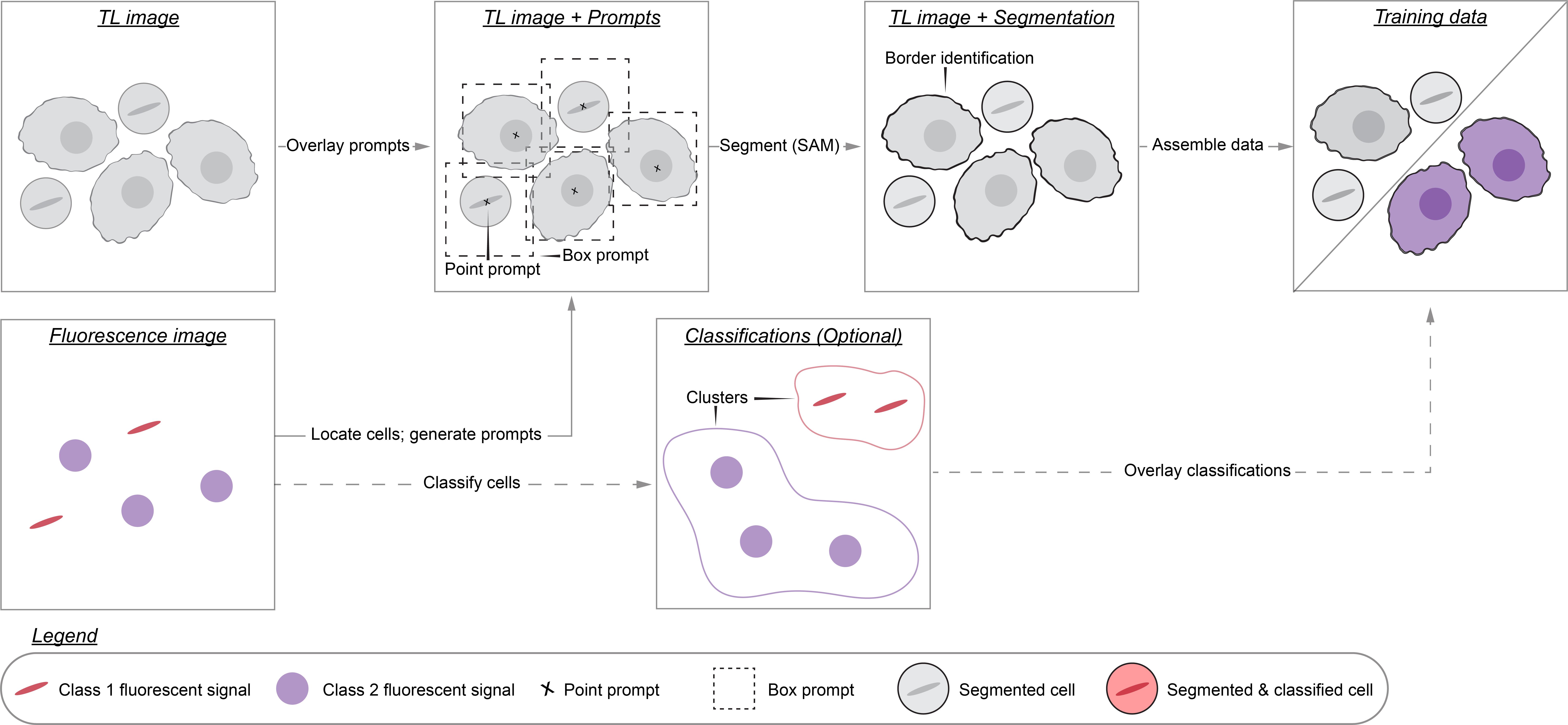
To this aim, we developed Cell-APP (cellular annotation and perception pipeline), a tool that automatically generates high-quality datasets for the training of deep learning–based models that segment adherent cells in transmitted-light (TL) microscopy images. With Cell-APP-generated datasets, users can build models tailored to their cell lines and imaging conditions. The tool requires only two inputs—paired TL and fluorescence images—and these inputs have a minimal set of requirements. First, signals in the fluorescence images must correspond to individual cells and be spatially separate from one another; this is because the fluorescence images are used to locate cells. Second, cells in the TL image must be non-overlapping and have discernible boundaries; if they do not, Cell-APP may produce erroneous cell outlines (see Figure 1 for example inputs and outputs). Finally, Cell-APP includes an optional classification module that uses fluorescence-derived features to label cells. These fluorescence-based classes must correspond to visual differences in the TL image; if they do not, the trained cell segmentation models may not learn to classify cells accurately (see Figure S1 for the full process diagram).
Here, we provide a step-by-step guide for using Cell-APP to build custom cell segmentation models. The guide covers (A) acquiring, or repurposing, microscopy data for Cell-APP, (B–E) generating training and testing datasets, (F) training Detectron2 models on the generated datasets, and (G) results interpretation, evaluating the generated datasets and trained models.
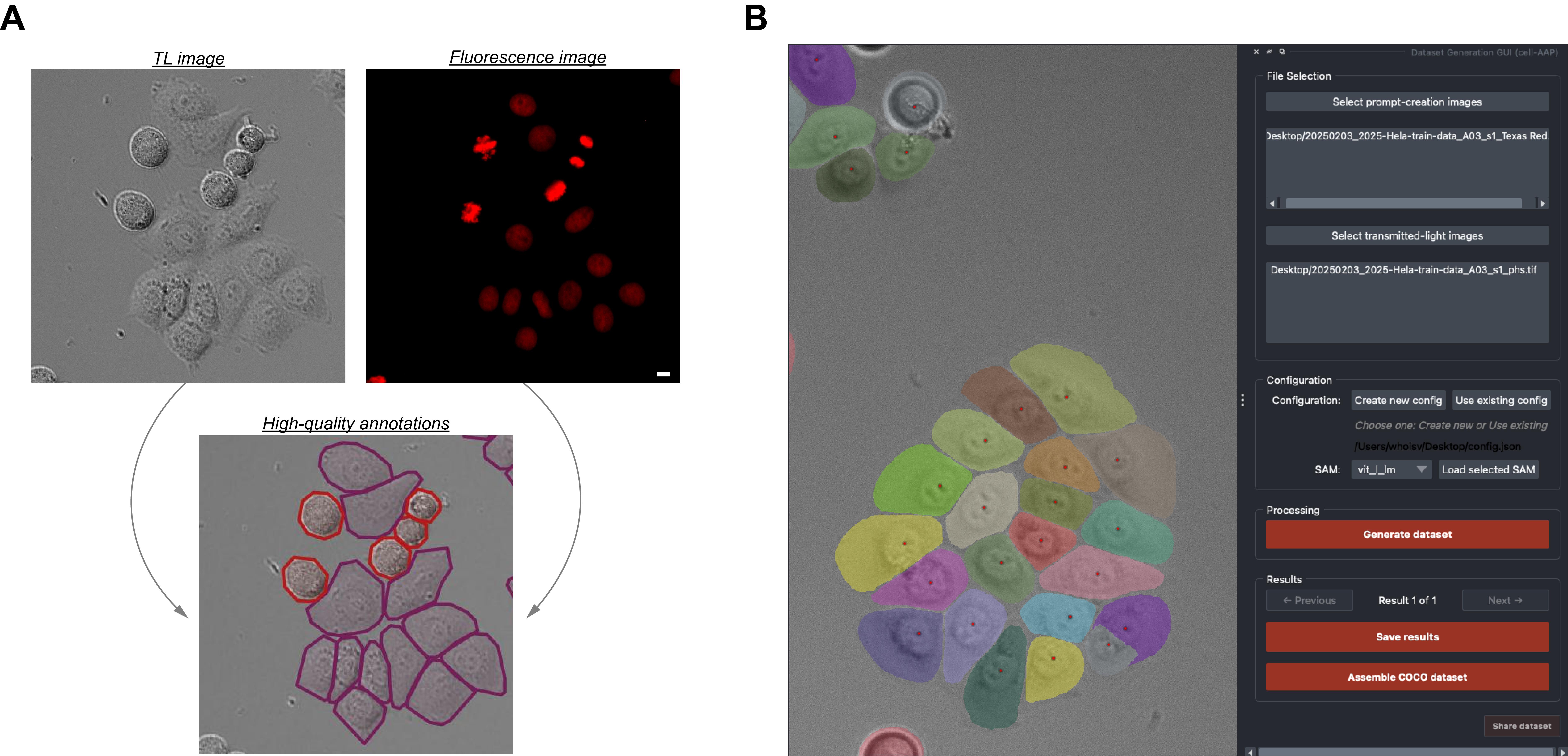
Figure 1. Input-output and Cell-APP graphical user interface examples. (A) Inputs (top row) and outputs (bottom row) that satisfy the described input requirements (see General note 1) and output standards (see Results Interpretation). (B) Example of the final segmentation results displayed within the Cell-APP graphical user interface. Scale bar = 10 μm.
Materials and reagents
Biological materials
1. One or more adherent, monolayered, metazoan cell lines (mycoplasma-free; expressing fluorescent protein or compatible with fluorescent dye for prompt creation). We used HeLa A12, hTERT-RPE1, U2OS, and HT1080 cell lines expressing Histone 2B-mCherry. We could have achieved equivalent results using unedited cell lines stained with SiR DNA dye (Cytochrome)
Reagents
1. Fetal bovine serum (Gibco, catalog number: 12657-029)
2. Penicillin–streptomycin solution (Thermo Fisher Scientific, catalog number: 15140122, or equivalent)
3. FluoroBriteTM DMEM (Thermo Fisher Scientific, Gibco, catalog number: A1896702)
4. DMEM (Thermo Fisher Scientific, Gibco, catalog number: 11960044)
5. HEPES (Thermo Fisher Scientific, Gibco, catalog number: 15630130)
6. GlutaMAXTM supplement (Thermo Fisher Scientific, Gibco, catalog number: 35050061)
7. (Optional) SiR-DNA (Spirochrome, Cytoskeleton, catalog number: CY-SC007)
8. (Optional) GSK923295 (Fisher Scientific, catalog number: 50-000-02189)
9. (Optional) Thymidine (Sigma-Aldrich, catalog number: T9250)
Solutions
1. Supplemented DMEM/FluoroBriteTM DMEM (see Recipes)
Recipes
1. Supplemented DMEM/FluoroBriteTM DMEM
| Reagent | Final concentration | Quantity or volume |
|---|---|---|
| DMEM or FluoroBriteTM | n/a | 500 mL |
| Fetal bovine serum | ~10% | 50 mL |
| 1 M HEPES | ~25 mM | 12.5 mL |
| GlutaMAXTM | ~1% | 5 mL |
| Penicillin–streptomycin solution | ~1% | 5 mL |
Laboratory supplies
1. 5 mL serological pipettes (Thermo Fisher Scientific, catalog number: 170355N)
2. 10 mL serological pipettes (Thermo Fisher Scientific, catalog number: 170356N)
3. BasixTM polypropylene conical centrifuge tubes (Fisher Scientific, catalog number: 14-955-237)
4. EppendorfTM safe-lock tubes 1.5 mL (microtube) (Fisher Scientific, catalog number: E0030123611)
5. CorningTM PrimariaTM tissue culture dishes (Fisher Scientific, catalog number: 08-772-4A)
6. μ-plate 96-well square (Ibidi, catalog number: 89626)
Equipment
1. For dataset generation: Computer with sufficient (C11) RAM or access to a high-performance computing cluster
2. (Optional) For model training: NVIDIA GPU-enabled computer or access to a high-performance computing cluster
3. (Optional) For data acquisition: Fluorescence-equipped microscope; we used an ImageXpress Nano Automated Imaging System equipped with a SOLA Light Engine and a 20×, 0.46 NA objective
Software and datasets
| Type | Software/dataset/resource | Version | Date | License | Access |
|---|---|---|---|---|---|
| Software 1 | cell-AAP | 1.0.7 | 1/7/2025 | MIT | Free |
| Software 2 | Detectron 2 | 0.6 | 11/15/2021 | Apache-2.0 | Free |
| Software 3 | Python | 3.11 | 10/24/2022 | PSFL | Free |
| Software 4 | Miniconda | Depends on the user’s computer | n/a | MEULA | Free |
Procedure
Please note: This is not a linear procedure. A is required only if you do not already have data that meets our input requirements (for requirements, see General note 1). After section C, sections D and E may be followed individually or in combination to generate training data; using section E enables Cell-APP’s classification functionality. Section F describes the use of one possible framework for training a cell segmentation model using your Cell-APP-generated dataset; other suitable frameworks exist.
A. Collecting microscopy data
Registered transmitted-light/fluorescence image pairs are the necessary inputs to Cell-APP. We recommend that you collect images according to the following instructions. If you have existing data that could be suitable for Cell-APP, see General note 1. The following instructions assume the following: (1) The cells you wish to image are mycoplasma-free and in 2D culture, and (2) the cells you wish to image are stably expressing a fluorescent marker that can be used to locate cells, or that you will be using a live-cell stain instead (see Figure S3 for example suitable and non-suitable fluorescent images).
1. Plate the cells in Supplemented DMEM; use a clear-bottom plate appropriate for your microscope(s).
Note: You should plate a quantity of cells such that at imaging time, you can comfortably image over 10,000 cells.
2. After the cells have adhered (adherence time depends on cell line), exchange their media with a low-fluorescence alternative (such as a supplemented or non-supplemented FluoroBriteTM).
3. Optionally prepare your cells for imaging.
a. If your cells are not expressing a fluorescent marker that can be used to locate cells, we recommend Spirochrome’s SiR-DNA. This live-cell stain can be used to visualize chromatin by following the manufacturer’s protocol. Chromatin fluorescence is suitable for Cell-APP to locate cells and classify them as mitotic or non-mitotic.
b. If your Cell-APP dataset will be used to train a model that classifies cells, ensure that each class is equally represented in the training set. To meet this condition, it may be necessary to stage the data acquisition process in a manner that increases the frequency of rare classes. As an example, in the original article describing Cell-APP, we trained models to classify cells as mitotic (rare) or non-mitotic (common). To partially remedy this class imbalance, we synchronized our cells via a single thymidine block and subsequently treated them with GSK923295, a mitotic poison. The poison lengthened the time our cells spent in mitosis, and the synchronization enabled us to image at a time when we expected an elevated mitotic index.
4. Acquire registered pairs of TL and fluorescence images.
Note: This process can be made significantly easier by using a semi-automated microscopy system. We used an ImageXpress Nano from Molecular Devices.
a. We recommend that at each selected plate position, you acquire three TL/fluorescence image pairs. In one pair, the TL image will be in focus; in another, the focus of the TL image will lie just above the “in focus” plane; in the last, the focus of the TL image will lie just below the “in focus” plane. The focus of the fluorescence image should remain “in focus” for each pair. This data augmentation will enable you to train your model on images with varying focus, which we have found to improve model robustness.
b. We recommend that you acquire images containing, in sum, at least 10,000 cells. These images should vary in confluency.
c. We recommend that you image any given group of cells (cells at a single plate position) no more than once (or three times if you consider the focus variants).
5. Ensure that (1) all images are in the TIFF or JPEG format, and (2) images within each TL-fluorescence image pair are saved as separate files. Images should be saved in either 8- or 16-bit unsigned integer or 32-bit float data types. We additionally recommend that all image dimensions are divisible by 16, e.g., 1,024 × 1,024. We make this recommendation as the transforms that happen during model training involve splitting the images into 16 × 16 patches. However, this is not a hard requirement, as the model training script can handle incorrectly sized images via padding.
B. Installing Cell-APP and Detectron 2
This protocol requires two main packages: Cell-APP and Detectron 2. Cell-APP houses the code for dataset generation; Detectron 2 is a package from Meta that facilitates model training. We recommend installing both Cell-APP and Detectron 2 in a clean Conda environment. In this environment, you should first install Detectron 2’s main dependency, PyTorch. Then, you can install Cell-APP from the Python Package Index and Detectron 2 from source. Installing Cell-APP will automatically install all its dependencies, which include scikit-image and Napari [7]. Detailed instructions and exact commands for installing Cell-APP and Detectron 2 can be found at https://github.com/anishjv/cell-AAP/tree/main.
C. Tuning dataset generation parameters in the Cell-APP graphical user interface
The method Cell-APP uses to locate cells in fluorescence images depends on a group of empirically chosen parameters. Choosing a suitable set of parameters may therefore require some trial and error. The Cell-APP graphical user interface (GUI) is optimal for this, as it allows you to choose parameters, run Cell-APP on subsets of your microscopy data, and visualize the results (images, prompts, and annotations). Below are instructions on using the GUI. Some examples of TL-fluorescence image pairs—which you may use to execute these instructions—can be found here: https://github.com/anishjv/cell-AAP/tree/main/notebooks/tutorials/dataset_generation/20250429-cellapp-data. Within this directory, TL images end in “phs.tif” and fluorescence images end in “Texas Red.tif.” To see how this section’s output should appear, see Figure S2.
1. Open your computer’s command-line interface and activate the conda environment in which you installed Cell-APP.
2. Type “napari” to open the GUI.
3. Once Napari is open, navigate to Plugins/Cell-APP/Dataset Generation GUI. This will open a panel on the left side of the Napari window (we recommend dragging it to the left if it opens up top).
4. Click Select prompt-creation images. This will open your computer’s file explorer, from which you should select a subset of your fluorescence images.
5. Click Select transmitted-light images. This will open your computer’s file explorer, from which you should select the TL images corresponding to the fluorescence images you picked in step C4.
Note: You must ensure that the ordering of the prompt-creation image list and transmitted-light image list matches. If they do not match, you may drag and drop file paths to re-order the lists.
6. First-time users click Create new config. This will once again open your file explorer, except this time, it will save a default Cell-APP configuration file at a location of your choosing. The configuration file is in YAML format. It will automatically open in your default text editor for inspection; you may close this window. We recommend that you apply the default configurations when first using Cell-APP. If you already have a configuration file, click Use existing config, and navigate to the file from the pop-up file explorer window.
7. Select a μSAM model from the dropdown menu labeled SAM: and click Load selected SAM. Models are available for both light microscopy (labeled “_lm”) and electron microscopy (labeled “_em”). There are three models for each modality, labeled as “vit_l,” “vit_b,” and “vit_t.” These names stand for Vision Transformer large, base, and tiny [8,9]. We recommend using the largest possible model in line with your computer’s capabilities; for example, data “vit_l_lm” fits this recommendation.
Note: The first time you load a given SAM model, it will be downloaded to your computer and will consume ~2 GB of storage; this may take some time.
8. Click Generate dataset. This will start Cell-APP dataset generation. You can monitor progress by viewing status messages in the terminal (Figure S4). After Cell-APP has finished, the results from one TL-fluorescence image pair will open in Napari. These results will consist of four images titled “Prompts (points or boxes),” “Prompt-creation image,” “Segmentations,” and “Transmitted-light image.” You can use the Next and Previous buttons near the bottom of the GUI to scroll through results from all TL-fluorescence image pairs.
9. To evaluate Cell-APP and determine which config-file parameters to modify, view Prompts (points or boxes) and Segmentations. Here is some guidance on what to look for:
a. In Prompts (points or boxes), you should ensure that each cell has exactly one prompt. If this is the case, no configurations need to be changed. If this is not the case, see General note 2 for guidance on parameter fine-tuning.
b. In Segmentations, you should ensure that each cell has a self-contained, high-quality segmentation. If this is the case, no configurations need to be changed. If this is not the case, see General note 3 for segmentation-specific guidance on parameter fine-tuning.
Note: You may need to hide the displayed fluorescence image to see the segmentations.
10. If you determined that parameters need to be adjusted, open the configuration file on your computer, make the necessary changes, and repeat steps C6–C10 until you are satisfied with the outputs.
D. Generating datasets with the Cell-APP graphical user interface
Having selected dataset-generation parameters that yield reasonable results (section C), you are now ready to run Cell-APP on all your microscopy data and generate your full dataset. If you have relatively few image pairs (under ~50, ~10 MB/image) or your computer has a large amount of RAM (over 50 GB), you may generate your dataset directly in the GUI. If you do not meet these criteria, you will need to generate your dataset on a high-performance computing cluster (HPC). In this case, we find it easier to generate datasets using Jupyter than using the GUI (section E). This is because the desktop-enabled nodes offered by HPCs often do not interface with our GUI. The following instructions are for generating datasets within the Cell-APP GUI.
1. Repeat steps C1–C8 using the transmitted light-fluorescence image pairs that you desire for your dataset.
2. After the dataset has been generated, use the Next and Previous buttons near the bottom of the GUI to scroll through the results and verify their quality.
3. Click Assemble COCO dataset to initiate dataset compilation. Once clicked, you will be asked to (1) name your dataset, (2) select the range of images to comprise your training dataset, (3) select the range of images to comprise your testing dataset, (4) select the range of images to comprise your validation dataset, and (5) name the class of objects in the dataset (usually “cell”).
Note: Selected ranges must not overlap. For example, if your dataset has two images and you want the first image to comprise the training dataset and the second to comprise the testing dataset, enter “0,0” for the training dataset range, “1, 1” for the testing dataset range, and “none” for the validation dataset range.
We recommend generating both a training and a testing dataset. In section F, the training dataset will be used to train your custom cell segmentation model; the testing dataset will be used to evaluate the model periodically during this training.
4. Once complete, a ZIP file containing the dataset will be saved to your desktop. The ZIP file should contain separate folders for each dataset you chose to create: testing, training, and/or validation. Within each of these folders, you should find a JSON file—this is the COCO-formatted dataset—and two folders named “annotations” and “images.” The folder named “annotations” should contain all individual cell masks in the dataset. The folder named “images” should contain all the transmitted light images in the dataset.
E. Generating datasets with Cell-APP in Jupyter
Dataset generation via Jupyter Notebook [10] is analogous to dataset generation via the GUI in that it consists of the same steps: selecting TL-fluorescence image pairs, choosing parameters, loading a μSAM model, generating, and finally, assembling the dataset. The key difference is that you will execute these steps by writing code, as opposed to clicking buttons. We recommend generating your dataset in Jupyter, rather than the GUI, if (1) you wish to classify instances in your dataset, or (2) if you must generate your dataset on an HPC because your computer lacks the necessary RAM (C11a). We have prepared an annotated Jupyter Notebook to guide you through this process: https://github.com/anishjv/cell-AAP/blob/main/notebooks/tutorials/dataset_generation/example.ipynb. Just as in section C, you may execute this Notebook using the example TL-fluorescent image pairs found here: https://github.com/anishjv/cell-AAP/tree/main/notebooks/tutorials/dataset_generation/20250429-cellapp-data. The optional mask classification section of the notebook will require additional data found here: https://github.com/anishjv/cell-AAP/tree/main/embeddings.
F. Training and evaluating custom Detectron 2 models
The dataset you generated in sections D or E is called, in the jargon of computer vision, COCO-format (Common Objects in Context-format) [11]. Datasets of this format can be used to train deep learning-based cell segmentation models using Meta AI’s object detection platform Detectron 2 [12,13]. The following instructions will guide you through this training process. You may follow these instructions using an example COCO-format dataset (found here: https://github.com/anishjv/cell-AAP/tree/main/notebooks/tutorials/training/example_dataset), which we created by applying the instructions in sections C/D to the example images provided in section C. We recommend that you train your model using a suitable NVIDIA GPU, which you may own outright or rent from an HPC.
1. Download the files “training.sh,” “training.py,” and “config.yaml” from https://github.com/anishjv/cell-AAP/tree/main/notebooks/tutorials/training. “training.py” registers your COCO-format dataset and initiates model training; “training.sh” is the bash script to run “training.py,” and “config.yaml” stores the necessary model configurations and training parameters.
2. Open the script “training.py” and modify the parameters at the top of the script. These parameters facilitate the registration of your COCO-format dataset and modify “config.yaml” for training. Guidance on modifying these parameters can be found within the script itself.
Note: The parameters built into “training.py” do not modify “config.yaml” in an exhaustive way. As downloaded, “config.yaml” is set up to train a Vision Transformer backboned model [14]. The model backbone and many other aspects of the configuration file—such as data augmentations, optimizer settings, learning rate schedule, and anchor sizes—can be further modified. To learn more about Detectron2 configuration files, see: https://detectron2.readthedocs.io/en/latest/tutorials/configs.html.
3. Run “training,py” by calling “python training.py” or “sh training.sh.” Once you do this, a file named “log.txt” will be generated in the output directory you specified within “training.py.” This file will summarize your model’s training in real-time.
G. Results interpretation
There are two points in the protocol where you should stop and evaluate your outputs. The first is during dataset generation (sections C, D, and E). Here, you should examine the annotations that Cell-APP is producing and determine if they are of sufficient quality (see Figure 1 for exemplary high-quality annotations). If you are using the Cell-APP GUI (section D), annotations will be displayed automatically after dataset generation. If you are using Jupyter (section E), you will have to visualize annotations programmatically; the tutorial demonstrates how to do this.
The second is after model training (section F). Here, you must (1) choose the optimal model weights for use in downstream cell segmentation, and (2) determine if those optimal weights are sufficient for your analysis needs. For (1), you should examine your model’s performance metrics: average precision (AP) and average recall (AR). You can find these metrics alongside your model’s weights in the previously mentioned “log.txt” file. These metrics will have been computed every n training epochs, where n is a period defined in the file “training.py.” For a detailed explanation of these metrics, see https://cocodataset.org/#detection-eval. During the course of model training, these performance metrics should increase and eventually plateau, which suggests that the model weights have converged to stable values. We have empirically found that picking the set of weights immediately after the plateau strikes a good balance between over- and under-fitting. We recommend that you use your selected weights to segment the images in your testing set and visualize the results. We have prepared a Jupyter Notebook demonstrating how to do such segmentation: https://github.com/anishjv/cell-AAP/tree/main/notebooks/tutorials/inference.
Validation of protocol
This protocol has been used and validated in the following research article:
• Virdi and Joglekar. [15]. Cell-APP: A generalizable method for cell annotation and cell-segmentation model training. Molecular Biology of the Cell, mbc. E25–02–0076.
General notes and troubleshooting
General notes
1. Cell-APP input requirements:
a. Cells in the TL images must have identifiable borders (Figure 1).
b. Cells in the fluorescence images must be spatially separate (Figure 1).
c. Cells in the TL images may partially overlap; however, a Cell-APP dataset created from such images will likely contain partial masks. In other words, μSAM will not infer the true border of a cell that is partially hidden beneath another cell; it will instead act as if that part of the cell does not exist.
d. TL-fluorescence image pairs must not be visually correlated (i.e., do not image the same cells under the same microscopy conditions more than once). Avoid overlapping images.
e. Images in your datasets must all be the same shape. We additionally recommend that all image dimensions are divisible by 16, e.g., 1,024 × 1,024.
f. Suggestion: It is best that image pairs for the training dataset and testing dataset come from different wells/plates. This eliminates the possibility of train-test contamination.
2. Here, we will walk users through all the parameters involved in locating cells within fluorescence images [16,17]. All parameters can be modified within the configuration file generated in step C6.
Note: The pipeline these parameters pertain to was engineered for segmenting images of chromatin. Locating cells in other kinds of fluorescence images may require you to use a different pipeline or even other deep learning models, such as StarDist or CellPose.
a. threshold_type: This parameter specifies the intensity thresholding algorithm. It can be set to “single,” in which case the Isodata algorithm will be used; “multi,” in which the Otsu’s algorithm with multiple bins will be used; or watershed, in which a distance-based watershed algorithm will be used. We recommend that you start with “single.” If you see that multiple cells are given one prompt centered on their collective centroid, you may try “watershed.” If you see that many cells are missing prompts and that your fluorescence image is of non-uniform intensity, you may try “multi.”
b. threshold division: This parameter exists to make the image thresholding more aggressive, which helps separate nearby cells. By default, it is set to 0.75. Values less than one make the thresholding more aggressive, while values greater than one make it less aggressive. If using “watershed” or “multi,” we recommend setting this parameter to 1. If you see that multiple cells are given one prompt centered on their collective centroid, you may decrease this parameter (we recommend decreasing in increments of 0.1). If you see that cells are missing prompts, you may increase this parameter.
c. gaussian_sigma: We apply a Gaussian filter before thresholding to reduce noise. We recommend that you compare your images to those in Figure 1. If your fluorescence images display relatively more or less Gaussian noise, you may adjust this parameter accordingly.
d. morphology: This group of parameters specifies optional image morphology operations that can be applied to enhance the thresholding.
i. tophatstruct: Here, you can choose to apply a white top-hat filter before thresholding. The white top-hat filter can be thought of as background subtraction and is therefore recommended if your images have a non-zero background. By default, we use a square kernel of side length 71. We recommend that you use square or rectangular kernels; kernels of other shapes are less efficient computationally. You may change the kernel size, but be sure that it is larger than the smallest object you intend to threshold.
ii. erosionstruct: Here, you can choose to apply image erosion before thresholding. The erosion operator separates connected objects whose connecting areas are smaller than the erosion kernel. By default, we use a disk kernel of radius 8. You may change the kernel size, but if you must use a large kernel (radius greater than 20 pixels), we recommend that you change the kernel shape to square or rectangular, as image erosion with disk kernels is computationally intensive.
3. Here, we will walk through all the parameters involved in annotating cells with μSAM.
a. point_prompts: This parameter is either “true” or “false” and determines if μSAM will be given each cell’s centroid.
Note: Only one of “point_prompts” and “box_prompts” should be “true.”
b. box_prompts: This parameter is either “true” or “false” and determines if μSAM will be given each cell’s bounding box.
Note: Only one of “point_prompts” and “box_prompts” should be “true.”
c. iou_thresh: This parameter operates after μSAM annotation and determines if any generated cell masks should be discarded. Cell-APP should be used to annotate images of 2D cell cultures. For this reason, cell masks should not overlap. Any cell masks with overlap (intersection-over-union) greater than that specified by “iou_thresh” will be discarded.
Supplementary information
The following supporting information can be downloaded here:
1. Figure S1. Dataset generation process diagram.
2. Figure S2. Expected dataset generation results.
3. Figure S3. Valid and invalid Cell-APP inputs.
4. Figure S4. Cell-APP dataset generation screen capture.
Acknowledgments
Conceptualization, A.J.V. and A.P.J.; Experimentation, A.J.V.; Writing of the original draft, A.J.V.; Reviewing and editing the paper, A.J.V. and A.P.J.; Funding acquisition, A.P.J.; Supervision, A.P.J. A.J.V. thanks Mishan Gagnon for always enjoyable and insightful conversations, including the one that introduced him to S.A.M. A.J.V. thanks Jennifer Guan for hand-annotating microscopy images in contribution to the original research article describing Cell-APP. Both A.J.V. and A.P.J. thank the entire Joglekar Lab for their support. This work was supported by R35- GM126983 to A.P.J. from the NIGMS. This protocol was used in [15].
Competing interests
The authors declare no competing interests.
References
- Stringer, C. and Pachitariu, M. (2025). Cellpose3: one-click image restoration for improved cellular segmentation. Nat Methods. 22(3): 592–599. https://doi.org/10.1038/s41592-025-02595-5
- Stringer, C., Wang, T., Michaelos, M. and Pachitariu, M. (2020). Cellpose: a generalist algorithm for cellular segmentation. Nat Methods. 18(1): 100–106. https://doi.org/10.1038/s41592-020-01018-x
- Fazeli, E., Roy, N. H., Follain, G., Laine, R. F., von Chamier, L., Hänninen, P. E., Eriksson, J. E., Tinevez, J. Y. and Jacquemet, G. (2020). Automated cell tracking using StarDist and TrackMate. F1000Res. 9: 1279. https://doi.org/10.1101/2020.09.22.306233
- Schmidt, U., Weigert, M., Broaddus, C. and Myers, G. (2018). Cell Detection with Star-Convex Polygons. In: Frangi, A., Schnabel, J., Davatzikos, C., Alberola-López, C., Fichtinger, G. (eds). Medical Image Computing and Computer Assisted Intervention – MICCAI 2018. MICCAI 2018. Lecture Notes in Computer Science. 265–273. https://doi.org/10.1007/978-3-030-00934-2_30
- Edlund, C., Jackson, T. R., Khalid, N., Bevan, N., Dale, T., Dengel, A., Ahmed, S., Trygg, J. and Sjögren, R. (2021). LIVECell—A large-scale dataset for label-free live cell segmentation. Nat Methods. 18(9): 1038–1045. https://doi.org/10.1038/s41592-021-01249-6
- Schwendy, M., Unger, R. E. and Parekh, S. H. (2020). EVICAN—a balanced dataset for algorithm development in cell and nucleus segmentation. Bioinformatics. 36(12): 3863–3870. https://doi.org/10.1093/bioinformatics/btaa225
- Contributors, n. (2019). napari: a multi-dimensional image viewer for python.
- Archit, A., Freckmann, L., Nair, S., Khalid, N., Hilt, P., Rajashekar, V., Freitag, M., Teuber, C., Spitzner, M., Tapia Contreras, C., et al. (2025). Segment Anything for Microscopy. Nat Methods. 22(3): 579–591. https://doi.org/10.1038/s41592-024-02580-4
- Kirillov, A., Mintun, E., Ravi, N., Mao, H., Rolland, C., Gustafson, L., Xiao, T., Whitehead, S., Berg, A. C. and Lo, W.-Y. (2023). Segment anything. Proceedings of the IEEE/CVF international conference on computer vision. 4015–4026. https://doi.org/10.1109/ICCV51070.2023.00371
- Kluyver, T., Ragan-Kelley, B., Pérez, F., Granger, B., Bussonnier, M., Frederic, J., Kelley, K., Hamrick, J., Grout, J. and Corlay, S. (2016). Jupyter Notebooks–a publishing format for reproducible computational workflows. Positioning and power in academic publishing: Players, agents and agendas. IOS Press. 87–90. https://doi.org/10.3233/978-1-61499-649-1-87
- Lin, T. Y., Maire, M., Belongie, S., Hays, J., Perona, P., Ramanan, D., Dollár, P. and Zitnick, C. L. (2014). Microsoft COCO: Common Objects in Context. In: Fleet, D., Pajdla, T., Schiele, B., Tuytelaars, T. (eds). Computer Vision – ECCV 2014. ECCV 2014. Lecture Notes in Computer Science. 8693: 740–755. https://doi.org/10.1007/978-3-319-10602-1_48
- Paszke, A., Gross, S., Massa, F., Lerer, A., Bradbury, J., Chanan, G., Killeen, T., Lin, Z., Gimelshein, N. and Antiga, L. (2019). Pytorch: An imperative style, high-performance deep learning library. Advances in neural information processing systems 32.
- Wu, Y., Kirillov, A., Massa, F., Lo, W.-Y., Girshick, R. (2019). Detectron2. (Accessed on)
- Li, Y., Mao, H., Girshick, R. and He, K. (2022). Exploring Plain Vision Transformer Backbones for Object Detection. In: Avidan, S., Brostow, G., Cissé, M., Farinella, G.M., Hassner, T. (eds). Computer Vision – ECCV 2022. ECCV 2022. Lecture Notes in Computer Science. 13669: 280–296. https://doi.org/10.1007/978-3-031-20077-9_17
- Virdi, A. J. and Joglekar, A. P. (2025). Cell-APP: A generalizable method for cell annotation and cell-segmentation model training. Mol Biol Cell. 36(11): ee25–02–0076. https://doi.org/10.1091/mbc.e25-02-0076
- Harris, C. R., Millman, K. J., van der Walt, S. J., Gommers, R., Virtanen, P., Cournapeau, D., Wieser, E., Taylor, J., Berg, S., Smith, N. J., et al. (2020). Array programming with NumPy. Nature. 585(7825): 357–362. https://doi.org/10.1038/s41586-020-2649-2
- van der Walt, S., Schönberger, J. L., Nunez-Iglesias, J., Boulogne, F., Warner, J. D., Yager, N., Gouillart, E. and Yu, T. (2014). scikit-image: image processing in Python. PeerJ. 2: e453. https://doi.org/10.7717/peerj.453
Article Information
Publication history
Received: Nov 3, 2025
Accepted: Jan 15, 2026
Available online: Feb 5, 2026
Published: Feb 20, 2026
Copyright
© 2026 The Author(s); This is an open access article under the CC BY-NC license (https://creativecommons.org/licenses/by-nc/4.0/).
How to cite
Readers should cite both the Bio-protocol article and the original research article where this protocol was used:
- Virdi, A. J. and Joglekar, A. P. (2026). How to Train Custom Cell Segmentation Models Using Cell-APP. Bio-protocol 16(4): e5618. DOI: 10.21769/BioProtoc.5618.
- Virdi, A. J. and Joglekar, A. P. (2025). Cell-APP: A generalizable method for cell annotation and cell-segmentation model training. Mol Biol Cell. 36(11): ee25–02–0076. https://doi.org/10.1091/mbc.e25-02-0076
Category
Bioinformatics and Computational Biology
Cell Biology > Cell imaging > Live-cell imaging
Cell Biology > Single cell analysis
Do you have any questions about this protocol?
Post your question to gather feedback from the community. We will also invite the authors of this article to respond.