- Protocols

- Articles and Issues
- For Authors
- About
- Become a Reviewer

A Quantitative DNA Fiber Assay to Monitor Replication Fork Progression, Protection, and Restart
Published: Vol 16, Iss 3, Feb 5, 2026 DOI: 10.21769/BioProtoc.5593 Views: 225
Reviewed by: Elena A. OstrakhovitchAnonymous reviewer(s)
Original research article
The authors used this protocol in:

Jun 2025

Protocol Collections
Comprehensive collections of detailed, peer-reviewed protocols focusing on specific topics


Abstract
Our genome is duplicated during every round of cell division through the process of DNA replication, but this fundamental process is subjected to various stresses arising from endogenous or exogenous sources. Thus, studying replication dynamics is crucial for understanding the mechanisms underlying genome duplication in physiological and replication stress conditions. Earlier, radioisotope-based autoradiography and density-labeling methods were used to study replication dynamics, which were limited in spatial resolution, representing only average estimates from many DNA samples. Here, we describe a DNA fiber assay that utilizes different thymidine analog incorporation, like 5-chloro-2’-deoxyuridine (CldU) and 5-iodo-2’-deoxyuridine (IdU), into replicating DNA. Such labeled DNA can be stretched and fixed on silanized glass slides, which are denatured with mild acidic treatment to expose the labeled nascent DNA. This DNA can then be visualized by using primary antibodies against CldU and IdU, followed by fluorophore-conjugated secondary antibodies, and observing them using a fluorescence microscope. The DNA fiber assay allows the visualization of individually replicating DNA at a single-molecular resolution and is highly quantitative, high-throughput, and easily reproducible. This technique offers insights into different replication parameters, like rate of DNA synthesis, extent of reversed fork protection, restart of stalled forks, and fork asymmetry under untreated or replication stress conditions at a single-molecule level.
Key features
• Single-molecule resolution of DNA replication dynamics.
• Diverse replication parameters can be quantified with variations of the labeling protocol.
• Easily reproducible across different cell lines in any lab with a basic molecular biology setup.
• Effective in studying the effects of different genotoxic treatments on replication.
Keywords: ReplicationGraphical overview
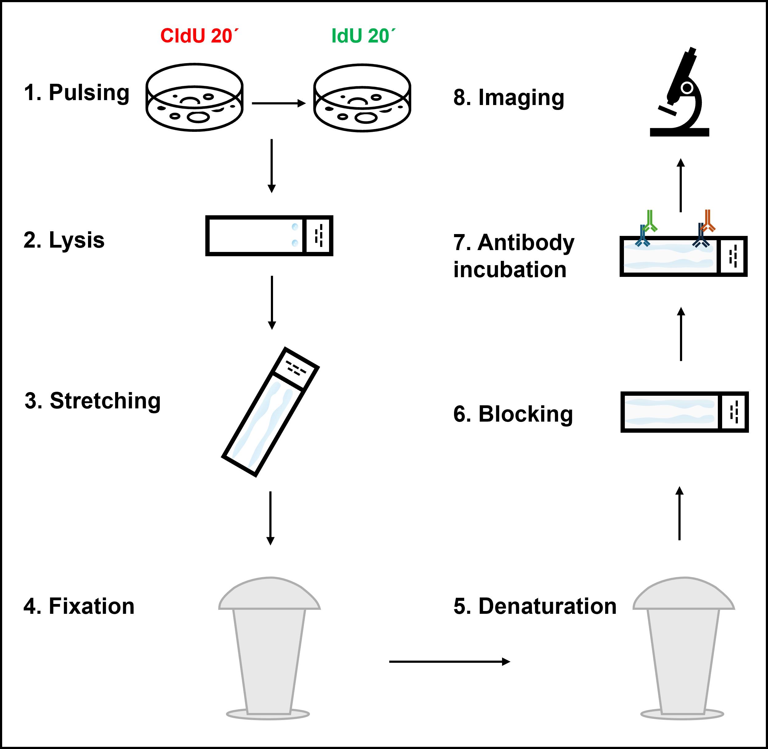
Graphical overview depicting the key steps of the DNA fiber assay protocol
Background
Faithful DNA replication is fundamental to the maintenance of genome integrity. During each S phase of the cell cycle, replication forks duplicate the entire genome through coordinated synthesis of leading and lagging strands. However, replication forks frequently encounter obstacles such as DNA lesions, DNA-protein crosslinks, secondary DNA structures, unscheduled R-loops, and repetitive DNA sequences that can deregulate replication speed and cause fork stalling or collapse. Cells have evolved different replication stress response mechanisms to protect stalled forks, prevent nascent DNA degradation, and ensure efficient fork restart once the stress is relieved. Understanding these dynamic replication responses requires experimental tools that can visualize and quantify replication forks with high spatial and temporal resolution [1–4]. Earlier methods to study DNA replication dynamics largely relied on population-level labeling approaches. Autoradiography using tritiated thymidine incorporation provided the first visualization of replicating DNA in eukaryotic cells but offered limited spatial resolution and required long exposure times [5,6]. Subsequently, 5-bromo-2’-deoxyuridine (BrdU) incorporation combined with immunofluorescence was widely used to mark replication foci and to determine the fraction of cells undergoing replication, but it could not resolve individual replication tracts [7,8]. Similarly, bulk density labeling or alkaline sucrose gradient sedimentation techniques provided only average replication rates without single-molecule resolution [9]. Electron microscopy (EM) is the only method that allows direct visualization of replication intermediates, but it is technically demanding, requires large amounts of purified DNA, and has limited throughput [10,11].
The DNA fiber assay was developed to overcome these limitations [12]. In this method, cells are sequentially pulse-labeled with halogenated nucleoside analogs such as 5-chloro-2’-deoxyuridine (CldU) and 5-iodo-2’-deoxyuridine (IdU), which incorporate into newly synthesized DNA during replication. The pulse-labeling scheme can be combined with the treatment of replication stress–inducing agents to study the effects of different genotoxic agents on replication. The cells are then harvested, lysed, and stretched on glass slides to expose the labeled DNA, and immunostained with antibodies specific to each thymidine analog, producing red and green fluorescent tracts corresponding to the first and second labeling periods, respectively. The tract lengths can subsequently be measured and used as a quantitative readout of different replication parameters like fork speed, stalling, or degradation, depending on the labeling scheme. The DNA fiber assay is highly versatile (Figure 1). Under unperturbed conditions, consecutive double labeling of cells with CldU and IdU for 20–30 min each, followed by measuring either CldU or IdU tract length, allows the estimation of replication fork speed (kb/min), which typically averages around 1 kb/min in mammalian cell lines. Shorter replication tract lengths indicate frequent fork stalling events, whereas an extended fiber length indicates unrestrained DNA replication [13,14]. Combining the second labeling pulse with a low dose of genotoxic agents enables measurement of fork stalling induced by specific replication barriers, e.g., low doses of camptothecin (CPT, 50–100 nM) as markers for R-loop induced fork stalling [15]. Sister-fork asymmetry, calculated as the ratio of the two sister-fork tract lengths extending from a common origin (green-red-green tracts), serves as another indicator of fork stalling. Fork asymmetry is measured by calculating the lengths of two green tracts on either side of an origin (red tract) and taking the ratio of the longer tract to the shorter one or vice-versa. Symmetric forks have a sister fork ratio close to 1, whereas asymmetric forks have a ratio </> 1; thus, the sister fork ratio can serve as an estimate of fork progression vs. stalling.
Fork reversal is a global response to replication stress, and reversed forks are susceptible to fork degradation. The fork protection assay is useful for studying the extent of fork protection and as a surrogate marker for fork reversal under replication stress [16,17]. In this assay, after the CldU and IdU pulses, cells are subjected to a prolonged period of hydroxyurea (HU) treatment (2–4 mM for 5 h). In the absence of fork protection, the second label is gradually degraded, resulting in shorter IdU tracts compared to CldU tracts. The extent of fork protection is then calculated using IdU to CldU ratios, where a ratio close to 1 indicates efficient fork protection and a ratio less than 1 indicates fork degradation. In a recent study, a variation of this assay has been used as a surrogate marker for fork reversal in cells, where replication stress (e.g., 150 nM CPT) during the second pulse slowed fork progression, reducing the CldU/IdU ratio, which is indicative of fork reversal in cells [18].
Reversed replication forks are restarted by homologous recombination (HR)-based or repriming-based restart mechanisms once the replication stress is alleviated [1,19]. The fork restart assay can be used to quantify the percentage of stalled and restarted replication forks, as well as the replication speed after fork restart. In this assay, typically, the first pulse (CldU, 20 min) is followed by 2 mM HU treatment for 2 h to stall the forks, and then the second pulse (IdU, 40 min) is given, during which fork restart occurs. Only red tracts or red followed by very short green tracts are considered to be stalled forks, whereas red tracts followed by longer green tracts are counted as restarted forks. New origin-firing events can also be quantified in this assay by measuring only green tracts, which represent origins fired during the second pulse duration. The percentage of stalled forks is calculated as red tracts/(red + red-green tracts) × 100, and restarted forks are calculated as 100 - percentage of stalled forks [20].
Replication stress is often associated with the formation of ssDNA gaps in the nascent DNA, which are termed as daughter-strand gaps (DSGs) [21]. These gaps can be scored by combining the S1 nuclease assay with the DNA fiber technique [12,22]. Here, cells are sequentially pulse-labeled and subjected to replication stress, followed by permeabilization of the cells with CSK buffer (10 min) and a 30 min incubation with S1 nuclease (20 U/mL) enzyme [23]. The S1 nuclease nicks the DNA strand opposite to the ssDNA gaps, creating double-strand breaks (DSBs). This results in shorter IdU tract lengths and reduced IdU/CldU ratios, which serve as a quantitative marker for DSGs. Overall, employing the different labeling schemes, the DNA fiber assay can be easily combined with specific gene knockdowns or inhibitor treatments to mechanistically dissect molecular pathways of fork protection and replication stress responses [24,25].
Compared with earlier approaches, the major advantage of the DNA fiber assay is that it provides single-molecule resolution and direct quantitative measurement of fork dynamics. By tweaking the pulse-labeling scheme, different fork metabolisms like fork speed, fork asymmetry, fork protection/reversal, fork restart, and DSGs can be quantified, thus allowing accurate assessment of replication dynamics under different stress conditions. Additionally, the assay requires relatively simple equipment and can be performed in most cell lines. The method also enables statistical analysis of hundreds of replication events within a single experiment, making it a robust technique. However, it has certain limitations. The efficiency is dependent on the uniformity of fiber labeling and spreading. The procedure is low-throughput and labor-intensive compared to automated microscopy-based replication assays, as a minimum of 200–300 individual fibers must be manually measured in each experiment across biological replicates [26]. Artifacts from fiber overlapping or overstretching can also occur. Despite these caveats, the DNA fiber assay remains one of the most powerful and versatile methods for studying DNA replication and fork metabolism at the single-molecule level [13,27].
A derivative of the DNA fiber assay is the DNA combing technique, which uses molecular combing to uniformly stretch the DNA on silanized slides. DNA combing allows controlled, parallel alignment of individual DNA fibers at a constant extension factor (≈2 kb/μm) as compared to conventional DNA fiber spreading, in which DNA is randomly distributed and variably stretched. This uniform stretching improves precision and allows determination of inter-origin distances [28]. This technique can also be combined with fluorescence in situ hybridization (FISH) to study replication dynamics at specific genomic loci [29]. Although the method requires a constant-speed combing device, which is not readily available everywhere, and careful control of DNA quality to prevent breakage, DNA combing offers enhanced precision and reproducibility for single-molecule analysis of replication [30].
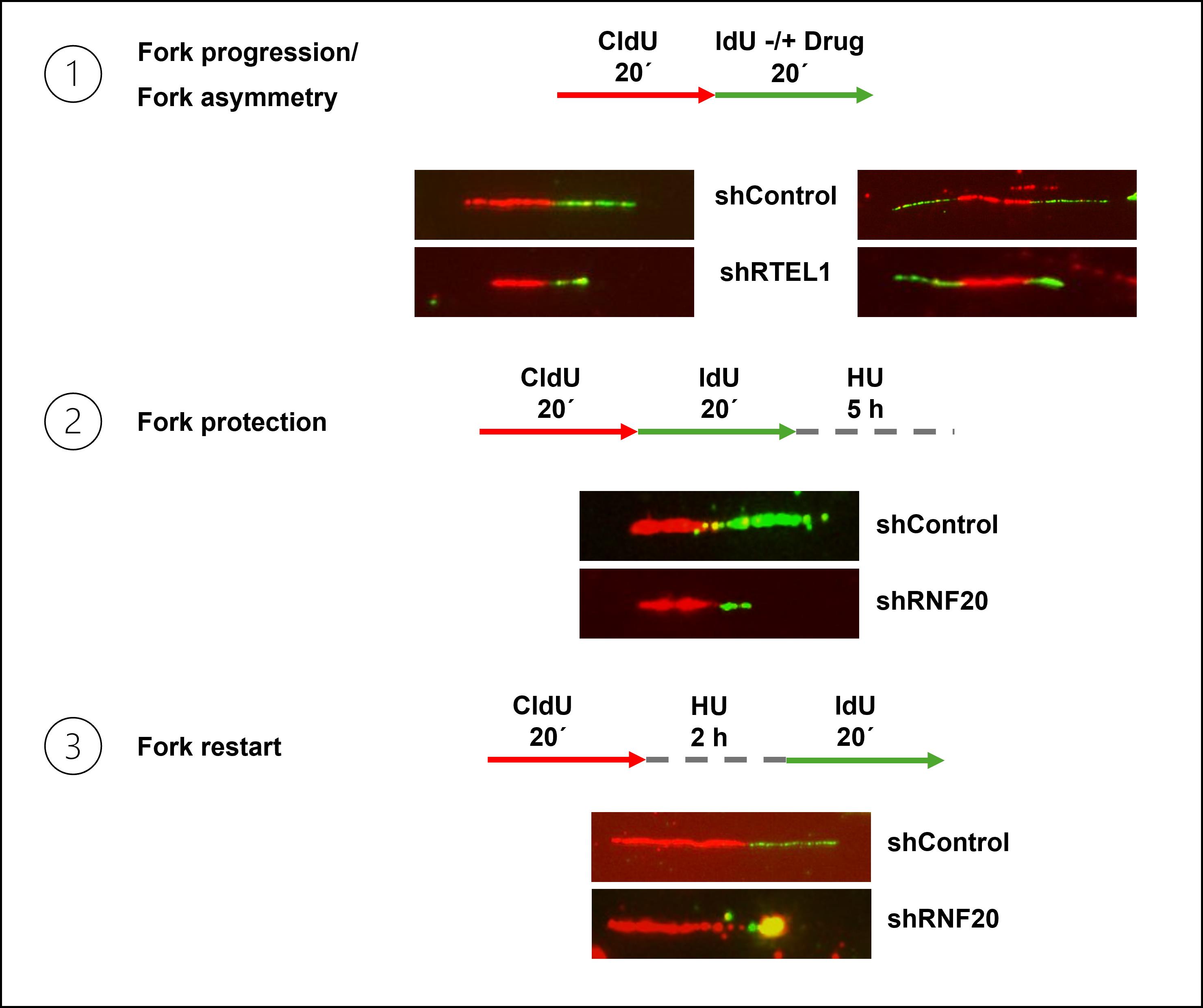
Figure 1. Representative images of different DNA fiber labeling schemes. 1: Schematic and representative fibers showing replication fork progression (left) and fork asymmetry (right) in control and RTEL1-depleted cells. 2: Schematic and representative fibers illustrating replication fork protection defect in RNF20-depleted cells compared with control cells. 3: Schematic and representative fibers from a fork restart assay demonstrating defective fork restart in RNF20-depleted cells relative to control.
Materials and reagents
Biological materials
1. U2OS cells (ATCC, catalog number: HTB-96; RRID:CVCL_0042)
Note: Cells were grown in DMEM medium supplemented with 10% FBS, 1% GlutaMax, and 1% PenStrep. Cells were regularly tested for mycoplasma with DAPI staining. Experiments were generally performed within 3rd–25th cell passages.
Reagents
1. 5-Chloro-2’-deoxyuridine (Sigma-Aldrich, catalog number: C6891)
2. 5-Iodo-2’-deoxyuridine (Sigma-Aldrich, catalog number: I7125)
3. Rat anti-BrdU (Abcam, catalog number: ab6326, RRID: AB_305426)
4. Purified mouse anti-BrdU (BD Biosciences, catalog number: 347580, RRID: AB_400326)
5. Donkey anti-rat Alexa Fluor 594 (Abcam, catalog number: ab150156, RRID: AB_2890252)
6. Rabbit anti-mouse IgG H&L Alexa Fluor 488 (Abcam, catalog number: ab150125)
7. Mowiol® 4-88 (Sigma-Aldrich, catalog number: 81381, CAS number: 9002-89-5)
8. Bovine serum albumin (BSA) (Sigma-Aldrich, catalog number: A7906, CAS number: 9048-46-8)
9. Hydroxyurea (Sigma-Aldrich, catalog number: H8627)
10. TWEEN® 20 (Sigma-Aldrich, catalog number: P1379)
11. Concentrated HCl (Qualigens, catalog number: Q29147)
12. Dimethyl sulphoxide (Sigma-Aldrich, catalog number: D8418)
13. Methanol (Sigma-Aldrich, catalog number: 6.06007, CAS number: 67-56-1)
14. Glacial acetic acid (Supelco, Merck, catalog number: 1.93002, CAS number: 64-19-7)
15. Trizma base (Sigma-Aldrich, catalog number: 93362)
16. Ethylenediaminetetraacetic acid (Sigma-Aldrich, catalog number: E6758)
17. Sodium dodecyl sulphate (Sigma-Aldrich, catalog number: 436143)
18. Trypsin-EDTA solution (Sigma-Aldrich, catalog number: T4174)
Solutions
1. Lysis buffer (see Recipes)
2. Blocking buffer (see Recipes)
3. Wash buffer (see Recipes)
4. CldU stock (see Recipes)
5. IdU stock (see Recipes)
6. Fixative (see Recipes)
7. HU stock (see Recipes)
Recipes
1. Lysis buffer
| Reagent | Final concentration | Quantity or volume |
|---|---|---|
| 1 M Tris-HCl (pH 7.5) | 0.2 M | 200 μL |
| 0.5 M EDTA (pH 8) | 0.05 M | 100 μL |
| 10% SDS | 0.5% | 50 μL |
| Autoclaved milli-Q water | n/a | 650 μL |
Filter-sterilize. It can be stored and used for a week at room temperature (RT).
2. Blocking buffer
| Reagent | Final concentration | Quantity or volume |
|---|---|---|
| BSA | 2% | 200 mg |
| Tween 20 | 0.1% | 10 μL |
| 1× PBS | n/a | up to 10 mL |
Filter-sterilize. It can be stored at 4 °C for 1–2 weeks.
3. Wash buffer
| Reagent | Final concentration | Quantity or volume |
|---|---|---|
| Tween 20 | 0.1% | 0.5 mL |
| 1× PBS | n/a | up to 500 mL |
It can be stored at RT for a few weeks.
4. CldU stock
| Reagent | Final concentration | Quantity or volume |
|---|---|---|
| CldU powder (262.65 g/mol) | 50 mM | 13.13 mg |
| Filter-sterilized, autoclaved milli-Q water | n/a | 1 mL |
Dissolve and store at -20 °C in 50 μL aliquots in the dark for up to 1 year, avoiding frequent freeze-thaw cycles.
5. IdU stock
| Reagent | Final concentration | Quantity or volume |
|---|---|---|
| IdU powder (354.1 g/mol) | 100 mM | 35.41 mg |
| Cell-culture grade DMSO | n/a | 1 mL |
Dissolve and store at -20 °C in 100 μL aliquots in the dark for up to 1 year, avoiding frequent freeze-thaw cycles.
6. Fixative
| Reagent | Final concentration | Quantity or volume |
|---|---|---|
| Methanol | 3 parts by volume | 37.5 mL |
| Glacial acetic acid | 1 part by volume | 12.5 mL |
Prepare fresh every time.
7. HU stock
| Reagent | Final concentration | Quantity or volume |
|---|---|---|
| Hydroxyurea powder | 200 mM | 15.212 mg |
| Filter-sterilized, autoclaved Milli-Q water | n/a | 1 mL |
Store at 4 °C for a couple of months in sealed aliquots.
Laboratory supplies
1. Superfrost slides (epredia/Fisher Scientific, catalog number: 16069901, Ref: AA00008032E01MNZ10)
2. Tissue culture 6-well plates (ThermoFisher, catalog number: 140675)
3. Cell counter or hemocytometer (ThermoFisher, model: Countess 3 Automated Cell Counter)
4. 1.5 mL microcentrifuge tubes (MCT) (Tarsons, catalog number: T500010)
5. 15/50 mL conical centrifuge tubes (Tarsons, catalog number: 546021/546041)
6. 15/50 mL centrifuge tube racks (Tarsons)
7. Coplin jars (local vendor)
8. 3-ply tissue paper (local vendor)
9. MCT rack (Tarsons, catalog number: 241010-B)
10. Whatman filter paper (GE Healthcare, catalog number: 1003-917)
11. Parafilm (PARAFILM, catalog number: 39209999)
12. Surface roller (local vendor)
13. Microscopic cover glass 24 × 60 mm (BLUE STAR)
14. 200–10,00 μL, 20–200 μL, 2–20 μL pipettes and pipette tips
Equipment
1. Fluorescence microscope (Zeiss AxioObserver)
2. Cell culture equipment, including CO2 incubator and biosafety chamber for culturing cells
Software and datasets
1. ImageJ (NIH, Version1.54p, Feb 2025, https://imagej.net/ij/download.htmL)
2. Microsoft Excel (Microsoft, https://products.office.com/en-us/excel)
3. GraphPad Prism (Version 9.5.1, graphpad.com/how-to-buy/)
Procedure
A. Pulse labeling (day 1)
Below, we describe the protocol for a fork protection assay using two samples with U2OS cells. Adjust pulse labeling scheme and reaction volumes of different reagents according to the type of experiment and the number of samples in the experiment, respectively.
1. After transfection with the desired shRNA/siRNA, seed cells into 6-well plates. If knockdown is not required, count 2.5 × 10⁵ cells and plate them in 6-well plates one day prior to the experiment. Plate 2.5 × 10⁵ plain U2OS cells in a 60 mm cell culture plate, separately for unlabeled cells.
Notes:
1. This experiment was performed using an electroporation-based transfection method. If using a different method for RNA-interference (e.g., Lipofectamine, DHARMAfect, etc.), perform gene knockdown according to the manufacturer’s protocol.
2. Cells should be approximately 80% confluent on the day of pulse labeling. Optimize the cell number for both unlabeled and labeled cells according to the cell line being used. Keep in mind that cell size and growth rate vary among different cell lines.
2. Prewarm cell culture media and PBS in a 37 °C water bath before starting pulse labeling. Thaw CldU and IdU aliquots at RT while incubating the media/PBS in the water bath. Depending on the ideal time point at which knockdown is achieved, start the pulse labeling scheme such that the pulse + damage treatment duration coincides with the duration of gene knockdown (e.g., we perform pulse labeling around 30 h after shRNA transfection, as we observe maximum depletion of our target protein 30 h post-transfection; for the fork protection assay, we perform pulse labeling at 27 h after transfection, followed by 5 h of HU damage). Prepare a 25 μM CldU solution in prewarmed media by adding 2.5 μL of CldU stock solution (50 mM) to 5 mL of media in a 15 mL centrifuge tube. Take out the 6-well plate containing your samples from the CO2 incubator and place it inside a biosafety cabinet. Aspirate the media and wash with 800 μL of 1× PBS. Aspirate the PBS and add 2 mL of the CldU mix to each sample in the 6-well plate. Place it back in the incubator and start your timer for 20 min (Table 1).
Caution: Ensure the media and PBS are pre-equilibrated to 37 °C before the pulsing step, as temperature changes can affect the labeling efficiency and quality of fibers.
Note: CldU preparation and pulsing step should be performed in the dark.
Table 1. Decision tree for choosing pulse labeling durations for DNA fiber assay depending on the replication speed of the cell line used. If the replication speed of the cell line being used is not known, a test experiment must be performed with a 15–20 min double labeling scheme, followed by tract length estimation of at least 100 individual fibers. The tract length can be converted to replication rate using the following formula: [(2.59 × measured tract length in μm)/ duration of pulse labeling in minutes]kb/min, where 1 μm = 2.59 kb.
| Fork speed (kb/min) | Suggested pulse duration | Notes |
|---|---|---|
| ≤0.5 kb/min (slow) | 30–45 min | Suitable for slow-dividing cell lines, e.g., primary cells. |
| 0.7–1.3 kb/min (typical mammalian) | 15–30 min (20 min default) | Works well for most common cell lines, e.g., U2OS, HeLa, HEK293, MCF7. |
| ≥1.5–2.0 kb/min (fast) | 5–15 min | Prevents excessively long or overlapping tracts in fast-replicating cells. |
3. During the incubation period, prepare 5 mL of 250 μM IdU solution by adding 12.5 μL of IdU (stock: 100 mM) to 5 mL prewarmed media. After 20 min, remove the plate from the incubator, aspirate the CldU-containing media, and wash three times with 800 μL of 1× PBS. Add 2 mL of IdU-containing media to each well and place it back in the incubator for 20 min.
Note: IdU preparation and pulsing should be performed in the dark.
4. During the incubation period, prepare 5 mL of 4 mM HU solution by adding 100 μL of HU (stock: 200 mM) to 5 mL of prewarmed media. After 20 min, take out the plate, aspirate the IdU-containing media, and wash three times with 800 μL of 1× PBS. Add 2 mL of 4 mM HU-media to each well and place them back in the incubator for 5 h.
B. Stretching (day 1)
5. After 5 h, take out the plate, aspirate the HU-containing media, and pour 3 mL of ice-cold PBS in each well to arrest the replication at that stage in the cells. Place the plate on ice in an ice bucket for 5 min. During this incubation period, take out the 60 mm plate of unlabeled U2OS cells, trypsinize it with 500 μL of trypsin (stock: 0.25×), add 500 μL of ice-cold PBS to neutralize the trypsin, and harvest it in a 1.5 mL microcentrifuge tube.
6. After 5 min, remove the 6-well plate from ice, aspirate the ice-cold PBS, and add 500 μL of prewarmed trypsin. Place it in the incubator for 3 min, add 500 μL of ice-cold PBS to stop the trypsinization process, harvest the samples in 1.5 mL microcentrifuge tubes, and place the tubes on ice.
7. Count the number of cells in each sample using a cell counter or hemocytometer if gene knockdown has been performed. It is essential to accurately estimate the cell numbers in each sample, as gene knockdown and transfection procedures can result in a significant amount of cell death. Note down the cell numbers of each sample.
8. Spin down the tubes at 7,000 rpm for 7 min at 4 °C.
9. Meanwhile, perform the following calculations: from the cell count, calculate the number of cells present in the total sample volume (1 mL in this case). Then, calculate the volume in which each sample should be resuspended to achieve a final dilution of 5 × 10⁵ cells/250 μL. Label a fresh set of 0.5 mL microcentrifuge tubes according to your samples and keep them on ice.
10. After centrifugation, discard the supernatant and resuspend the cell pellet thoroughly in an appropriate volume of ice-cold PBS according to the calculation done in step B9.
11. Transfer 10 μL of the unlabeled cell sample to each new 0.5 mL microcentrifuge tube and then add 20 μL of the labeled samples to their respective tubes, such that the labeled to unlabeled ratio in the new mixture is 2:1. Mix by pipetting thoroughly.
Note: The labeled to unlabeled cells ratio may need to be optimized depending on whether fibers are too dense or too sparse in the final images (See troubleshooting).
12. Clean the required number of superfrost slides, label them, and place them flat on top of a piece of tissue paper. Place a centrifuge tube rack near the top end of the slides (labeled side) and place them in the orientation shown in Figure 2.
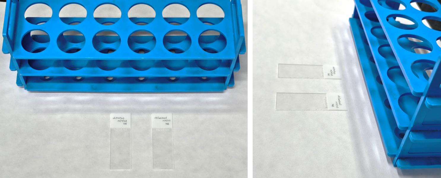
Figure 2. Position of slide placement for lysis. Lay the cleaned superfrost slides flat on top of tissue paper near a centrifuge tube rack with the labeled end of the slide toward the stand.
13. Add two drops of 7 μL of lysis buffer on each slide at a sufficient distance from each other such that the drops do not mix with each other (Figure 3).
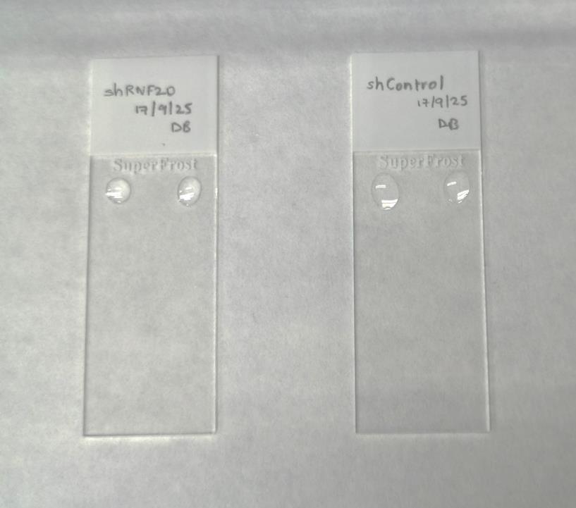
Figure 3. Lysis. Place two drops of lysis buffer on each slide, as shown in the image.
14. Take the first sample and mix it by tapping the end of the microcentrifuge tube and pipetting up and down. Then, add 3 μL of the sample to each dot of the lysis buffer on the slide, lightly swirling the mixture five times. Mix the sample with the lysis buffer thoroughly by pipetting up and down 8–12 times on the slide. Start the timer for 7–9 min. Repeat the same process for each sample.
Critical: Do this step as uniformly as possible across all samples, as it greatly affects the quality of fibers obtained in the final step. Ensure your tip is not touching your slide while swirling/mixing the sample. See Troubleshooting.
15. Once the sample is sufficiently lysed (approximately 7–9 min), raise the labeled end of the slide and balance it at an angle on the centrifuge tube rack kept next to it, as shown in Figure 4. This allows the sample to flow down on the slide in a continuous stream facilitated by the action of gravity. Allow each slide to stand for 10 min, so that it becomes sufficiently dry.
Caution: Air conditioners or fans should be turned off during this step; otherwise, the samples will dry up during the lysis period.
Note: If the cell suspension does not flow down naturally after lifting the slide, add 5 μL of lysis buffer on top of the sample drop to aid its flow.
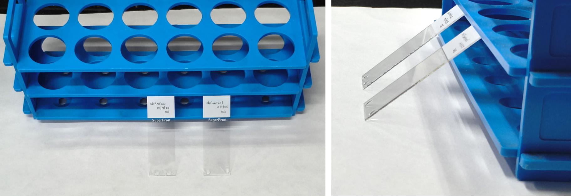
Figure 4. Fiber stretching. To stretch the fibers, raise each slide by hand and keep it at an angle, balancing on a centrifuge tube rack as shown.
16. Place the slides in 40 mL of fixative solution in a Coplin jar and keep them at 4 °C overnight.
Pause point: The slides can be stored in the fixative solution at 4 °C for 1–3 days.
Note: Acetic acid and methanol should be handled inside a chemical fume hood. During fixation, ensure that Coplin jars are tightly sealed with their lids to prevent evaporation and escape of acetic acid/methanol fumes. In the event of a spill, absorb the material immediately with spill pads, dispose of it in designated waste bins, and thoroughly wipe the surface with 70% ethanol. Avoid using open flames and ensure proper ventilation at all times.
C. Staining (day 2)
17. On the following day, take out the Coplin jar containing the slides from 4 °C, discard the fixative solution, and wash three times with 1× PBS, each time for 5 min, in the Coplin jar.
Caution: Ensure the fixative is thoroughly washed out by rinsing the Coplin jars with ample amounts of Milli-Q water, as this can interfere with the later steps.
Note: Between each wash, take out the slides from the Coplin jar and keep them tilted on a centrifuge tube rack on top of some tissue paper (position as shown in Figure 4).
18. Prepare a 2.5 M HCl solution for denaturation by mixing 10.4 mL of concentrated HCl (12 M) with 39.6 mL of autoclaved Milli-Q water in a SCHOTT DURAN bottle during the washes. Remove PBS from the Coplin jar after the final wash and add the denaturation solution. Incubate for 1 h at RT.
Caution: Prepare a 2.5 M HCl solution fresh each time, taking proper precautions.
19. After denaturation, wash the slides three times with PBS, for 5 min each wash, to neutralize the pH.
Note: Ensure the pH has been restored to 7 by checking the pH of the PBS in the final wash with a pH strip.
20. Prepare a humid chamber during the wash incubations. Place a blotting paper on top of a microcentrifuge tube rack and wet it with Milli-Q water. Use a roller to flatten the surface of the wet blotting paper and place a layer of parafilm on top of the paper. Flatten the surface again using the roller. Line the edges of the rack with a thin line of wet tissue paper. Cover the lid of the microcentrifuge tube rack with aluminum foil to protect the samples from light exposure, and then close the lid of the rack (Figure 5). Prepare this setup before the end of the PBS washes.
21. Drain the excess PBS from the slides after the last wash and lay the slides flat in the prepared humid chamber with the side containing the stretched fibers facing up. Add 100 μL of blocking solution on top of each slide and cover each slide with a piece of parafilm, ensuring there are no bubbles between the slide and the parafilm. Cover with lid and incubate for 45 min at RT. See Figure 5.
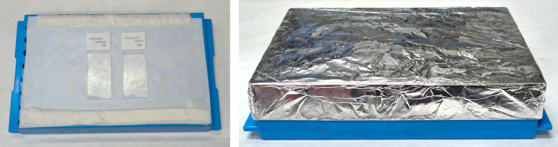
Figure 5. Setup for blocking and antibody incubations. Place the slides in the wet chamber, add the required quantity of blocking buffer/antibody solution on top of the slides, and cover with small pieces of Parafilm, ensuring there are no air bubbles. Cover the lid of the chamber with aluminum foil to make it light-proof and place the cover on top. Incubate for the required time.
22. During the blocking incubation, prepare the primary and secondary antibody dilutions and store them temporarily at 4 °C. For the primary antibody, dilute the rat anti-BrdU (for CldU) at a 1:500 dilution and the purified mouse anti-BrdU (for IdU) at a 1:250 dilution in blocking buffer. For two slides, add 0.3 μL of anti-CldU antibody and 0.6 μL of anti-IdU antibody to 150 μL of blocking buffer. For the secondary antibody, add 0.3 μL of both donkey anti-rat Alexa Fluor 594 (1:500) and rabbit anti-mouse IgG H&L Alexa Fluor 488 (1:500) to 150 μL of blocking solution.
23. After blocking, remove the parafilm pieces and keep them aside on a piece of tissue paper. Remove the excess blocking solution from the slides and add 60 μL of primary antibody mix to the slides. Place the parafilm pieces back on the slides, ensuring there are no bubbles. Close the lid and incubate for 2.5 h at RT.
24. After primary antibody incubation, wash the slides three times for 5 min with wash buffer in Coplin jars.
25. After draining off the excess wash buffer, place the slides in the wet chamber again as before (Figure 5) and add 60 μL of secondary antibody solution. Cover them with parafilm, place the lid on top to prevent exposure to light, and incubate for 1 h at RT.
Caution: This step is light sensitive.
26. Wash the slides three times for 5 min each with wash buffer in Coplin jars.
Caution: Protect from light exposure.
27. Keep the slides in a slanted position on the centrifuge tube rack and cover them to prevent light exposure. Allow slides to dry completely by leaving them at RT for 30 min.
28. Clean the microscope cover glasses carefully to ensure they are free of any dust. Lay the slide flat on a bench and add 15 μL of Mowiol mounting medium along one of the long edges of the slide. Place the coverslip along the same edge of the slide and lower it down gradually to ensure there are no bubbles between the slide and the coverslip. Leave the slides overnight at RT in a light-protected container for drying.
Notes:
1. If air bubbles form, press down on the coverslip and push it out through the closest edge of the slide.
2. If you are using a different mounting medium than Mowiol that remains in a liquid state after drying, seal the edges of the coverslip with nail polish.
29. Image the slides on the next day or store them in a slide box at 4 °C for a few weeks. Slides can be kept at -20 °C for long-term storage.
D. Imaging (day 3)
1. This step varies according to the microscope you are using. To locate the focus of the DNA fibers, find a field that shows fluorescent speckles. Your fibers will be on the same plane as these fluorescent dots. Next, move the objective lens along the width of the slide to find fibers as shown in Figure 6. Once the fibers are visible, move the objective lens along the length of the slide and capture a sufficient number of images.
Note: The images in Figure 6 have been acquired with a Zeiss AxioObserver microscope with a 63× oil-immersion objective lens. Representative data is presented in Figure 7.
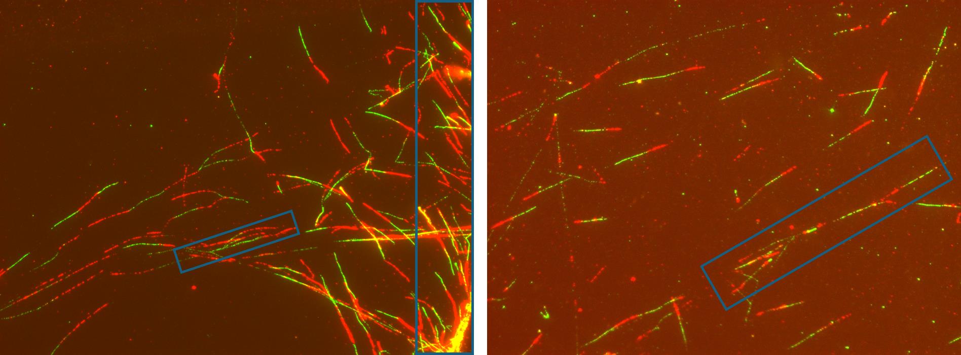
Figure 6. Raw images of fiber spreads prepared using this protocol. The blue boxes in the images indicate regions of clustered and overlapping fibers. During calculations, such areas of the fiber spread should be avoided, and only clearly distinguishable fibers should be counted to get accurate results.
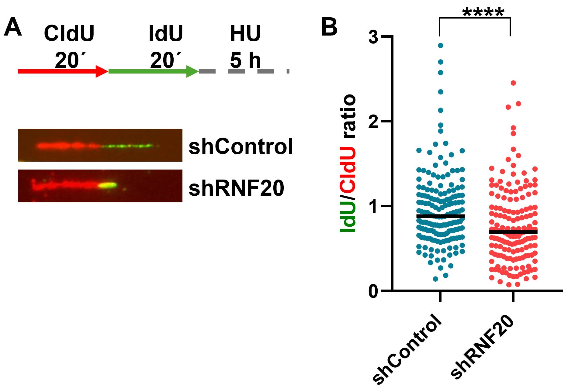
Figure 7. Example of a fork protection assay performed in control and RNF20-depleted U2OS cells. (A) Schematic outline of the fork protection assay (top) and representative fibers showing fork protection defect in control vs. RNF20-depleted cells (bottom). (B) Quantitative scatterplot of fibers as shown in A. Data represents the median value. ≥150 fibers were counted for each sample from three biological replicates. ****p(shControl vs. shRNF20) < 0.0001.
E. Quality control criteria
For each condition, ≥150 individual fibers were quantified across three biological replicates of an experiment. A fiber was considered analyzable if it displayed (i) continuous stretching (1 μm ≈ 2.5 kb), (ii) uninterrupted CldU/IdU tracts, (iii) no major breaks or dye diffusion (patchy appearance), (iv) distinct CldU and IdU tracts without extended overlap at the junctions, and (v) individual fiber not lying in an area of overlapped/clustered fibers.
In control samples, the expected length of IdU or CldU tracts is within 5–10 μm for U2OS cells with a 20-min pulsing time (replication rate in U2OS averages around 1 kb/min; the length of the labeled tract depends upon the replication rate of the cell line being used and the pulsing time). The number of fibers counted in an experiment varies between publications, with ≥100 fibers (from three repeats) being accepted in some publications. In general, 200–300 individual fibers should be counted from three independent biological replicates of an experiment.
Notes:
1. For fork asymmetry experiments, a total of ≥50 fibers is acceptable from three independent replicates of an experiment, since origin firing events are comparatively rare to find in DNA fiber spreads.
2. To prevent measurement bias, sample identifiers should be blinded during imaging and quantification, and conditions should be unblinded only after completing all measurements and proceeding to statistical analysis.
Data analysis
1. Set image scale
a. Open an image that includes a scale bar acquired using the same microscope objective used for capturing your experimental images.
b. Zoom into the scale bar area, select the line tool, and draw a straight line along the length of the scale bar (see Figure 8).
c. Click on Analyze--Set Scale. Enter the Known distance, Unit of length, and check the Global option. Click Ok (see Figure 8). Now your images are calibrated to the appropriate scale.
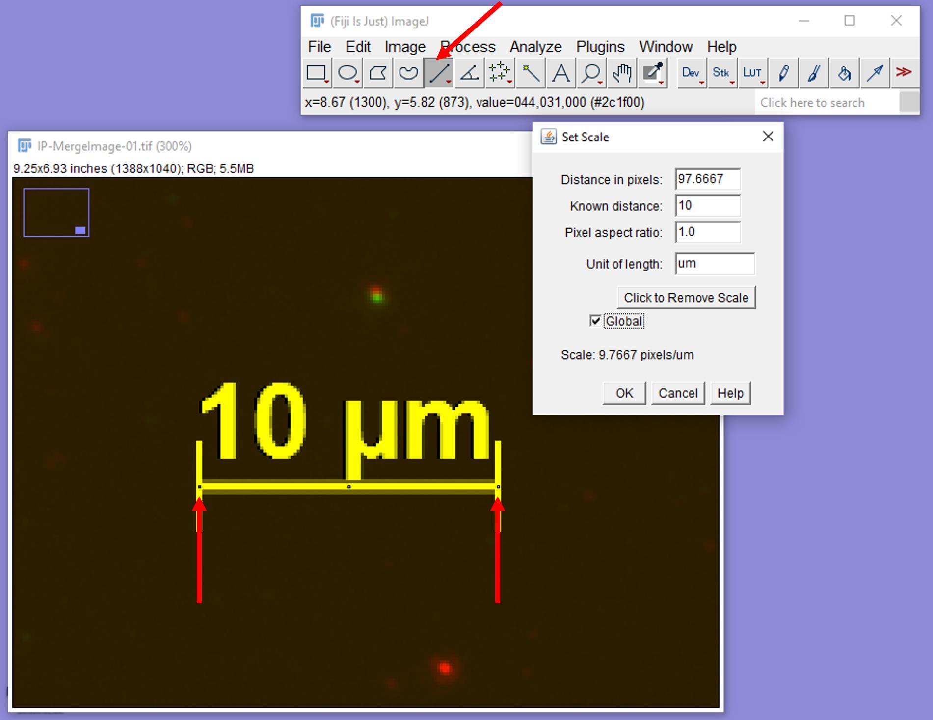
Figure 8. Setting the image scale. Zoom into the scale bar area and draw a straight line across the length of the scale bar by using the line tool, as shown with red arrows. Go to Analyze and Set Scale and enter the required values to calibrate the distance in pixels to the known length of the scale bar.
2. Calculating fiber length
a. To calculate the length of IdU or CldU tracts, open the image in ImageJ. Zoom into the area where the fibers are well-separated and clearly visible (Figure 9A, B).
b. Select the line tool and draw a straight line across the length of the CldU or IdU tract.
c. To select the measurement parameters you need, go to Analyze > Set Measurements, select the measurements you want to record, such as length, and deselect any you do not need, and then click Ok. Go to Analyze > Measure (Press M on your keyboard). A dialogue box called Results will appear, showing the value of the length measured with the line tool (Figure 9C).
Note: In case of fork protection assay, measure both CldU and IdU lengths one after another.
Caution: Remember to maintain the same order of measurement (i.e., CldU first and IdU second or vice-versa) throughout the entire calculation.
d. After measuring a sufficient number of fibers, copy and paste the data onto a blank Excel sheet. Delete any values other than the Length column.
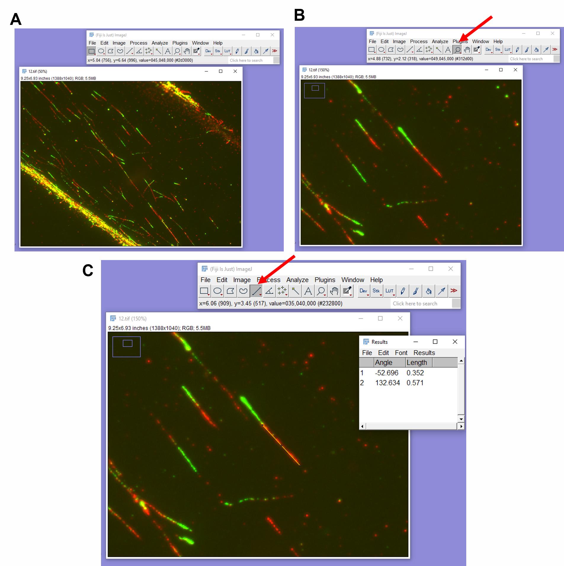
Figure 9. Measuring the length of the fibers. (A) Open your image in ImageJ. (B) Zoom into the area where fibers are well separated. (C) Select the line tool, draw a straight line across IdU or CldU length of a fiber, and press M on the keyboard. The Results tab will appear.
3. Calculating IdU to CldU ratios
a. Label the column containing your length measurements as Values. Label the adjacent column as Function (Figure 10A).
b. In the first cell of the Function column (next to your first length value), type the following formula:
=ISODD(ROW(select the cell containing the first length value)) (Figure 10A). Press Enter.
c. The cell will display either TRUE or FALSE, depending on whether the row number is odd or even. Extend the formula to all remaining rows by dragging the fill handle downward (bottom-right corner of the first cell) (Figure 10B).
d. Select the cell containing the column header “Function.” Click on Data in the menu bar, followed by the Filter option. A downward arrow will now appear on the right side of the “Function” header, indicating that a filter has been applied to it (Figure 10C).
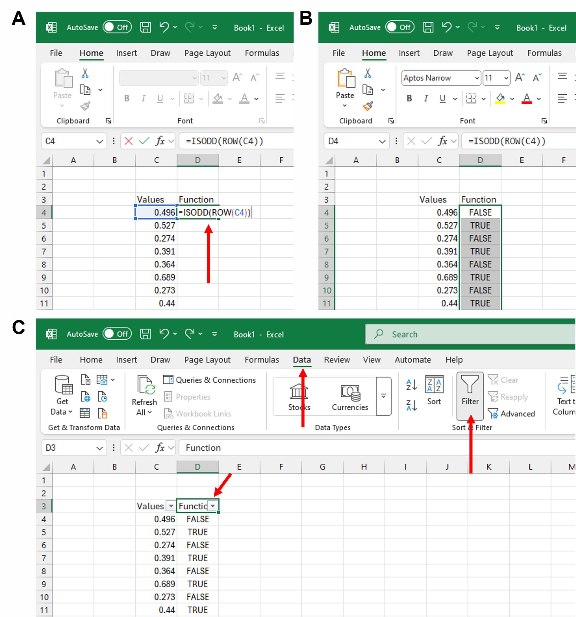
Figure 10. Calculating IdU to CldU ratios (part 1). (A) Paste your length values in a column in an Excel sheet and give a heading to the rows as shown. In the first cell under the “Function” header, type the formula as shown. (B) Extend the formula to all the rows containing “Values” by dragging the fill-in option. (C) Apply a filter to the “Function” header by clicking the Data tab, followed by the Filter option.
e. Click on the downward arrow in the “Function” cell. If the first data point corresponds to false, select the FALSE option under the Select all heading and click Ok (Figure 11A).
f. Now, only the rows corresponding to FALSE will be displayed. This will correspond to either CldU or IdU length values, depending on which one was measured first. Select all the FALSE rows and copy and paste them onto a fresh Excel sheet in a column labeled as CldU or IdU (Figure 11B, D).
g. Repeat the process for the TRUE values to isolate the second set of tract lengths and copy/paste them in the adjacent row of your first set of values in the new Excel sheet (Figure 11C, D).
h. Calculate the IdU to CldU ratio using the formula: = (select first IdU cell)/(select first CldU cell) and press Enter. Extend the formula to the remaining rows by dragging the fill-in handle at the bottom right corner of the first cell (Figure 11D).
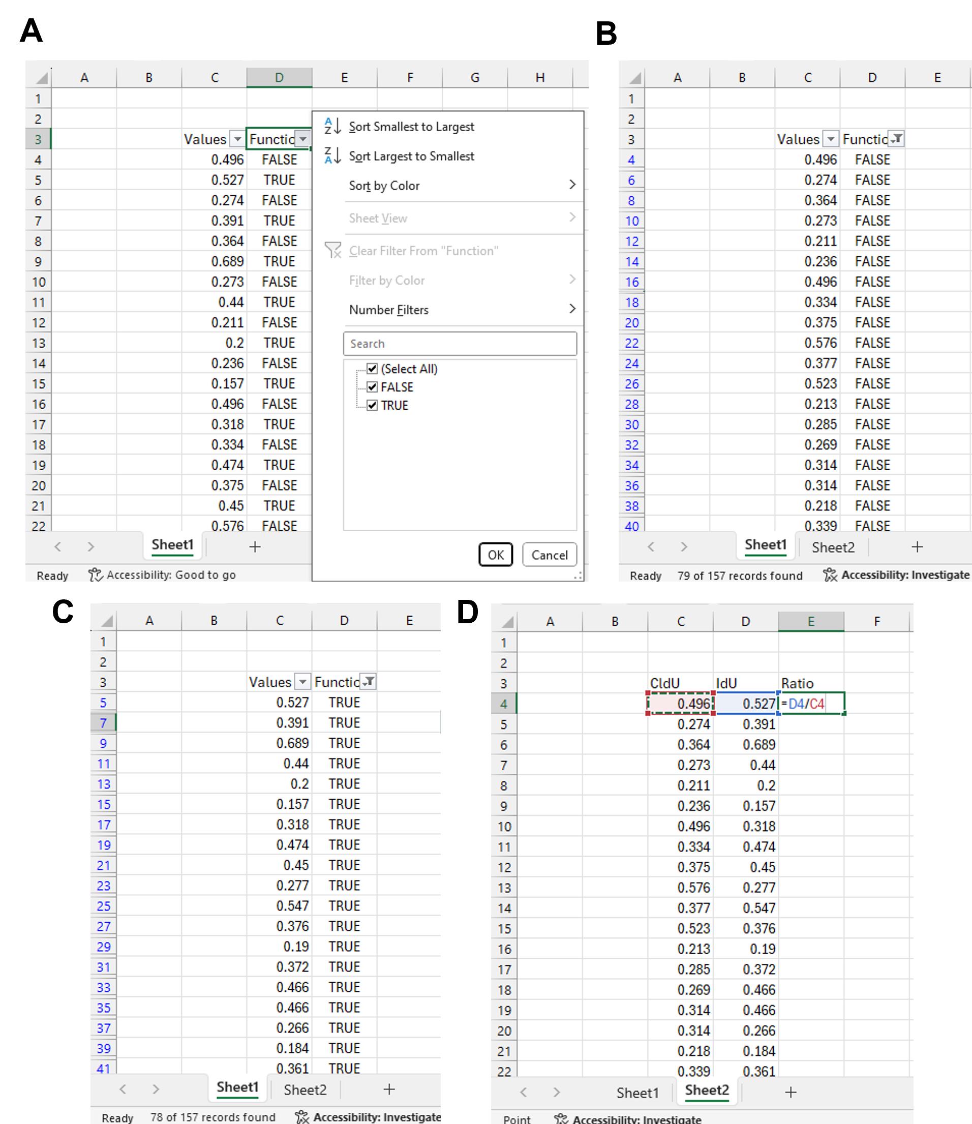
Figure 11. Calculating IdU to CldU ratios (part 2). (A) Click the arrow on the right side of the “Function” header and select FALSE in the select section. (B) Copy and paste all the numerical values under the “Values” header onto a fresh Excel sheet. All these values correspond to FALSE and, in turn, correspond to either CldU or IdU length, depending on which was measured first. (C) Click the arrow on the right side of the “Function” header and select TRUE in the select section. Copy and paste all the numerical values under the “Values” header corresponding to TRUE onto the fresh Excel sheet. (D) Calculate the IdU to CldU ratio using the formula as shown. Extend the formula to the remaining rows.
4. Plotting the data using Prism
a. Open Prism and choose the Column graph type under the Create option. Select Enter replicate values, stacked into columns under the Options menu.
b. A blank spreadsheet will open. Enter the names of the columns in the column headers according to your samples. Copy and paste the numerical values (e.g., IdU/CldU ratio, replication rate, etc.) of each sample from the Excel file onto the Prism spreadsheet (Figure 12A).
c. Click the datasheet under the Graphs option in the left-hand side menu. Select the Individual values, Scatter plot, and Median options. Click Ok (Figure 12B).
d. Edit graph settings like axes length, color, symbols, etc., according to your choice (Figure 12C).
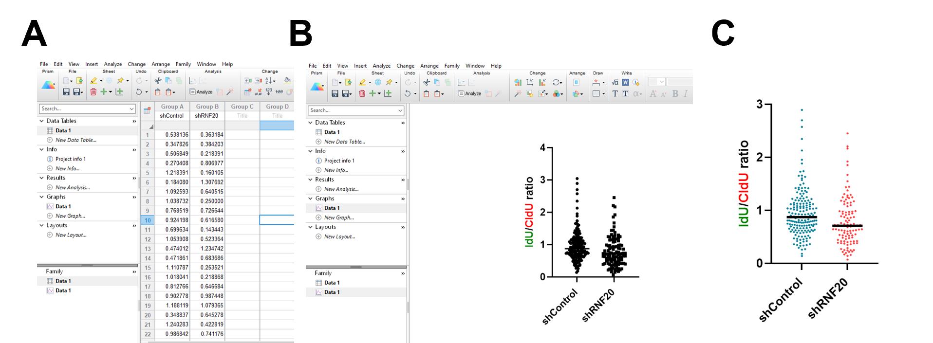
Figure 12. Plotting the data. (A) Copy/paste your data into a blank Prism file in the appropriate columns. (B) Select Data1 under Graphs and use individual data points to create a scatter plot. (C) Decorate the graph according to your choice.
5. Calculating statistical significance
a. Select the Analyze option as shown in Figure 13A.
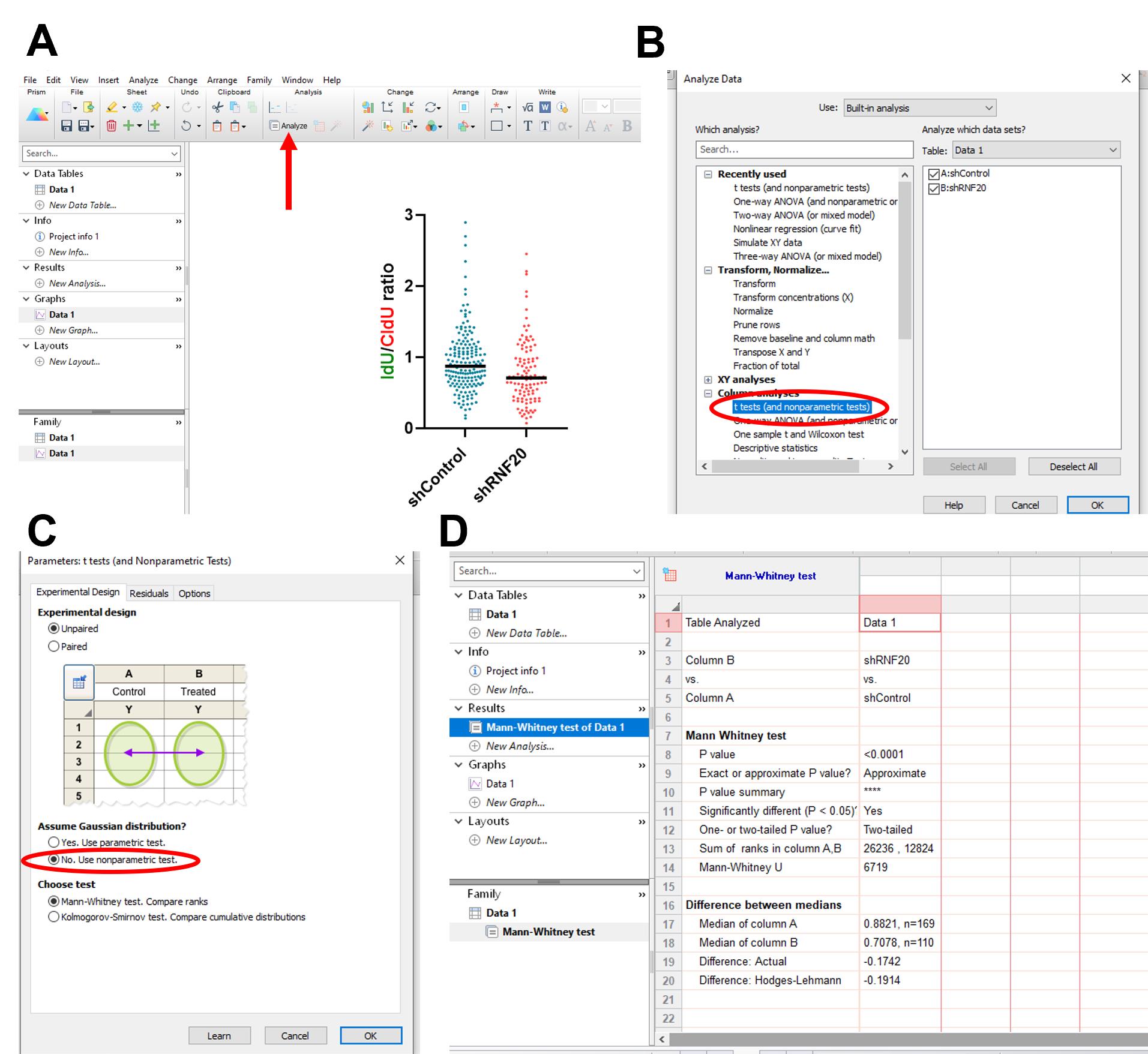
Figure 13. Calculating the statistical significance between different samples in the dataset. (A) Select Analyze. (B) Select t tests and your samples. (C) Click the nonparametric test option under Unpaired t test. (D) View the statistical calculations under the Results tab.
b. Select t tests under Column analyses. Select the two groups you wish to compare in the right-hand panel. If there are more than two groups, compare pairwise as many times as needed. Click Ok (Figure 13B).
c. Under Experimental design, select Unpaired t test. Under Assume Gaussian distribution? select No. Use nonparametric test. Under Choose test, select Mann-Whitney test. Click Ok (Figure 13C).
d. In the left-hand panel, under the Results section, click on the datasheet. The results of the t-test with all parameters measured are given here (Figure 13D).
e. You can add the significance between samples manually using whichever software you use to prepare your data figures (e.g., Microsoft PowerPoint or Adobe Illustrator). Otherwise, you can add significance between samples using the Draw option in Prism, followed by selecting Automatically add pairwise comparisons or Manually add lines with text options.
Validation of protocol
This protocol has been used and validated in the following research article:
Debanjali et al. [25] RNF20-mediated H2B monoubiquitination protects stalled forks from degradation and promotes fork restart. EMBO reports (Figure 3A–I; Figure 4A–B; Figure 5C–F, I–J; Figure 6D–F).
General notes and troubleshooting
Troubleshooting
Problem 1: Fibers appear degraded.
Possible cause: Excess lysis.
Solutions: Reduce the lysis time and perform the mixing/swirling step gently.
Problem 2: No fibers can be found on the slides.
Possible cause: Cells are unhealthy.
Solutions: Repeat the experiment with a fresh set of cells. Ensure cell culture conditions are optimal before starting the experiment.
Problem 3: Too much fluorescence background in the form of red or green dots in the imaging fields.
Possible causes: Nonspecificity of the antibody or insufficient washing.
Solutions: Reduce antibody concentration, add an extra wash step after primary and secondary antibody incubations, or add an extra blocking step for 15 min before secondary antibody incubation.
Problem 4: Fibers appear faint or discontinuous.
Possible cause: Insufficient antibody binding.
Solution: Increase the concentration of the primary antibodies.
Problem 5: Fibers are too dense or too sparse to be calculated.
Possible causes: Improper cell counting or insufficient spreading out of fibers during lysis.
Solution: If the fibers are too clumped together, try increasing the unlabeled cells in the sample mixture. If the fibers are too sparse, decrease or omit the mixing of unlabeled cells with labeled cells before lysis.
Acknowledgments
The conceptualization, investigation, and writing of the original draft of the manuscript was done by D.B. Review and editing of the manuscript, funding acquisition, and supervision was done by G.N. We thank Harsh Kumar Dwivedi for proofreading the manuscript. We thank Funding by Department of Science and Technology (EMR/2015/001720; CRG/2022/003533), Department of Atomic Energy (58/14/03/2022-BRNS), Department of Biotechnology (BT/PR23498/BRB/10/1590/2017; BT/PR45508/MED/30/2414/2022), Council of Scientific and Industrial Research (CSIR) (37/1756/23/EMR-II), JC Bose fellowship (JCB/2021/000009), IISc-DBT partnership program (BT/PR27952/INF/22/212/2018), and infrastructure support provided by funding from DST-FIST and UGC. D.B. was supported by a fellowship from the Department of Science and Technology, Indian Institute of Science, and JC Bose fellowship. This protocol has also been used in Dixit et al., 2024, and Nagraj et al., 2025 [31,32].
Competing interests
The authors declare no conflicts of interest.
References
- Petermann, E. and Helleday, T. (2010). Pathways of mammalian replication fork restart. Nat Rev Mol Cell Biol. 11(10): 683–687. https://doi.org/10.1038/nrm2974
- Neelsen, K. J. and Lopes, M. (2015). Replication fork reversal in eukaryotes: from dead end to dynamic response. Nat Rev Mol Cell Biol. 16(4): 207–220. https://doi.org/10.1038/nrm3935
- Berti, M., Cortez, D. and Lopes, M. (2020). The plasticity of DNA replication forks in response to clinically relevant genotoxic stress. Nat Rev Mol Cell Biol. 21(10): 633–651. https://doi.org/10.1038/s41580-020-0257-5
- Bhattacharya, D., Sahoo, S., Nagraj, T., Dixit, S., Dwivedi, H. K. and Nagaraju, G. (2022). RAD51 paralogs: Expanding roles in replication stress responses and repair. Curr Opin Pharmacol. 67: 102313. https://doi.org/10.1016/j.coph.2022.102313
- Taylor, J. H., Woods, P. S. and Hughes, W. L. (1957). The Organization and Duplication of Chromosomes as Revealed by Autoradiographic Studies Using Tritium-Labeled Thymidinee. Proc Natl Acad Sci USA. 43(1): 122–128. https://doi.org/10.1073/pnas.43.1.122
- Huberman, J. A. and Riggs, A. D. (1968). On the mechanism of DNA replication in mammalian chromosomes. J Mol Biol. 32(2): 327–341. https://doi.org/10.1016/0022-2836(68)90013-2
- Kennedy, B. K., Barbie, D. A., Classon, M., Dyson, N. and Harlow, E. (2000). Nuclear organization of DNA replication in primary mammalian cells. Genes Dev. 14(22): 2855–2868. https://doi.org/10.1101/gad.842600
- Leonhardt, H., Rahn, H. P., Weinzierl, P., Sporbert, A., Cremer, T., Zink, D. and Cardoso, M. C. (2000). Dynamics of DNA Replication Factories in Living Cells. J Cell Biol. 149(2): 271–280. https://doi.org/10.1083/jcb.149.2.271
- Raschke, S., Guan, J. and Iliakis, G. (2009). Application of Alkaline Sucrose Gradient Centrifugation in the Analysis of DNA Replication After DNA Damage. Methods Mol Biol. 521: 329–342. https://doi.org/10.1007/978-1-60327-815-7_18
- Zellweger, R. and Lopes, M. (2017). Dynamic Architecture of Eukaryotic DNA Replication Forks In Vivo, Visualized by Electron Microscopy. Methods Mol Biol. 1672: 261–294. https://doi.org/10.1007/978-1-4939-7306-4_19
- Sogo, J. M., Lopes, M. and Foiani, M. (2002). Fork Reversal and ssDNA Accumulation at Stalled Replication Forks Owing to Checkpoint Defects. Science. 297(5581): 599–602. https://doi.org/10.1126/science.1074023
- Quinet, A., Carvajal-Maldonado, D., Lemacon, D. and Vindigni, A. (2017). DNA Fiber Analysis: Mind the Gap!. Meth Enzymol. 591: 55–82. https://doi.org/10.1016/bs.mie.2017.03.019
- Técher, H., Koundrioukoff, S., Azar, D., Wilhelm, T., Carignon, S., Brison, O., Debatisse, M. and Le Tallec, B. (2013). Replication Dynamics: Biases and Robustness of DNA Fiber Analysis. J Mol Biol. 425(23): 4845–4855. https://doi.org/10.1016/j.jmb.2013.03.040
- Dhar, S., Datta, A., Banerjee, T. and Brosh, R. M. (2019). Single-Molecule DNA Fiber Analyses to Characterize Replication Fork Dynamics in Living Cells. Methods Mol Biol. 1999: 307–318. https://doi.org/10.1007/978-1-4939-9500-4_21
- Chappidi, N., Nascakova, Z., Boleslavska, B., Zellweger, R., Isik, E., Andrs, M., Menon, S., Dobrovolna, J., Balbo Pogliano, C., Matos, J., et al. (2020). Fork Cleavage-Religation Cycle and Active Transcription Mediate Replication Restart after Fork Stalling at Co-transcriptional R-Loops. Mol Cell. 77(3): 528–541.e8. https://doi.org/10.1016/j.molcel.2019.10.026
- Mijic, S., Zellweger, R., Chappidi, N., Berti, M., Jacobs, K., Mutreja, K., Ursich, S., Ray Chaudhuri, A., Nussenzweig, A., Janscak, P., et al. (2017). Replication fork reversal triggers fork degradation in BRCA2-defective cells. Nat Commun. 8(1): 859. https://doi.org/10.1038/s41467-017-01164-5
- Tye, S., Ronson, G. E. and Morris, J. R. (2021). A fork in the road: Where homologous recombination and stalled replication fork protection part ways. Semin Cell Dev Biol. 113: 14–26. https://doi.org/10.1016/j.semcdb.2020.07.004
- Longo, M. A., Roy, S., Chen, Y., Tomaszowski, K. H., Arvai, A. S., Pepper, J. T., Boisvert, R. A., Kunnimalaiyaan, S., Keshvani, C., Schild, D., et al. (2023). RAD51C-XRCC3 structure and cancer patient mutations define DNA replication roles. Nat Commun. 14(1): e1038/s41467–023–40096–1. https://doi.org/10.1038/s41467-023-40096-1
- Bainbridge, L. J., Teague, R. and Doherty, A. J. (2021). Repriming DNA synthesis: an intrinsic restart pathway that maintains efficient genome replication. Nucleic Acids Res. 49(9): 4831–4847. https://doi.org/10.1093/nar/gkab176
- Saxena, S., Somyajit, K. and Nagaraju, G. (2018). XRCC2 Regulates Replication Fork Progression during dNTP Alterations. Cell Rep. 25(12): 3273–3282.e6. https://doi.org/10.1016/j.celrep.2018.11.085
- Nagaraju, G. and Scully, R. (2007). Minding the gap: The underground functions of BRCA1 and BRCA2 at stalled replication forks. DNA Repair. 6(7): 1018–1031. https://doi.org/10.1016/j.dnarep.2007.02.020
- Cong, K., Peng, M., Kousholt, A. N., Lee, W. T. C., Lee, S., Nayak, S., Krais, J., VanderVere-Carozza, P. S., Pawelczak, K. S., Calvo, J., et al. (2021). Replication gaps are a key determinant of PARP inhibitor synthetic lethality with BRCA deficiency. Mol Cell. 81(15): 3227. https://doi.org/10.1016/j.molcel.2021.07.015
- Saxena, S., Dixit, S., Somyajit, K. and Nagaraju, G. (2019). ATR Signaling Uncouples the Role of RAD51 Paralogs in Homologous Recombination and Replication Stress Response. Cell Rep. 29(3): 551–559.e4. https://doi.org/10.1016/j.celrep.2019.09.008
- Schlacher, K., Christ, N., Siaud, N., Egashira, A., Wu, H. and Jasin, M. (2011). Double-Strand Break Repair-Independent Role for BRCA2 in Blocking Stalled Replication Fork Degradation by MRE11. Cell. 145(6): 993. https://doi.org/10.1016/j.cell.2011.05.021
- Bhattacharya, D., Dwivedi, H. K. and Nagaraju, G. (2025). RNF20-mediated H2B monoubiquitination protects stalled forks from degradation and promotes fork restart. EMBO Rep. 26(15): 3773–3803. https://doi.org/10.1038/s44319-025-00497-3
- Li, L., Kolinjivadi, A. M., Ong, K. H., Young, D. M., Marini, G. P. L., Chan, S. H., Chong, S. T., Chew, E. L., Lu, H., Gole, L., et al. (2022). Automatic DNA replication tract measurement to assess replication and repair dynamics at the single-molecule level. Bioinformatics. 38(18): 4395–4402. https://doi.org/10.1093/bioinformatics/btac533
- Liu, W. (2021). Single Molecular Resolution to Monitor DNA Replication Fork Dynamics upon Stress by DNA Fiber Assay. Bio Protoc. 11(24): e4269. https://doi.org/10.21769/bioprotoc.4269
- Meroni, A., Wells, S. E., Fonseca, C., Ray Chaudhuri, A., Caldecott, K. W. and Vindigni, A. (2024). DNA combing versus DNA spreading and the separation of sister chromatids. J Cell Biol. 223(4): e202305082. https://doi.org/10.1083/jcb.202305082
- Gali, H., Mason-Osann, E. and Flynn, R. L. (2019). Direct Visualization of DNA Replication at Telomeres Using DNA Fiber Combing Combined with Telomere FISH. Methods Mol Biol. 1999: 319–325. https://doi.org/10.1007/978-1-4939-9500-4_22
- Moore, G., Jimenez Sainz, J. and Jensen, R. B. (2022). DNA fiber combing protocol using in-house reagents and coverslips to analyze replication fork dynamics in mammalian cells. STAR Protoc. 3(2): 101371. https://doi.org/10.1016/j.xpro.2022.101371
- Dixit, S., Nagraj, T., Bhattacharya, D., Saxena, S., Sahoo, S., Chittela, R. K., Somyajit, K. and Nagaraju, G. (2024). RTEL1 helicase counteracts RAD51-mediated homologous recombination and fork reversal to safeguard replicating genomes. Cell Rep. 43(8): 114594. https://doi.org/10.1016/j.celrep.2024.114594
- Nagraj, T., Sahoo, S., Kadupatil, S. and Nagaraju, G. (2025). Distinct roles of RECQL5 in RAD51-mediated fork reversal and transcription elongation. Nucleic Acids Res. 53(19): e1093/nar/gkaf1019. https://doi.org/10.1093/nar/gkaf1019
Article Information
Publication history
Received: Oct 27, 2025
Accepted: Dec 25, 2025
Available online: Jan 13, 2026
Published: Feb 5, 2026
Copyright
© 2026 The Author(s); This is an open access article under the CC BY-NC license (https://creativecommons.org/licenses/by-nc/4.0/).
How to cite
Bhattacharya, D. and Nagaraju, G. (2026). A Quantitative DNA Fiber Assay to Monitor Replication Fork Progression, Protection, and Restart. Bio-protocol 16(3): e5593. DOI: 10.21769/BioProtoc.5593.
Category
Cancer Biology > Genome instability & mutation > Cell biology assays > DNA structure and alterations
Molecular Biology > DNA > DNA damage and repair
Do you have any questions about this protocol?
Post your question to gather feedback from the community. We will also invite the authors of this article to respond.