- Protocols

- Articles and Issues
- For Authors
- About
- Become a Reviewer

High Content In Vitro Survival Assay of Cortical Neurons
(*contributed equally to this work) Published: Vol 16, Iss 3, Feb 5, 2026 DOI: 10.21769/BioProtoc.5582 Views: 129
Reviewed by: Anonymous reviewer(s)

Protocol Collections
Comprehensive collections of detailed, peer-reviewed protocols focusing on specific topics


Abstract
Neuronal survival in vitro is usually used as a parameter to assess the effect of drug treatments or genetic manipulation in a disease condition. Easy and inexpensive protocols based on neuronal metabolism, such as 3-(4,5-dimethylthiazol-2-yl)-2,5-diphenyltetrazolium bromide (MTT), provide a global view of protective or toxic effects but do not allow for the monitoring of cell survival at the single neuronal level over time. By utilizing live imaging microscopy with a high-throughput microscope, we monitored transduced primary cortical neurons from 7–21 days in vitro (DIV) at the single neuronal level. We established a semi-automated analysis pipeline that incorporates data stratification to minimize the misleading impact of neuronal trophic effects due to plating variability; here, we provide all the necessary commands to reproduce it.
Key features
• The protocol enables monitoring of primary cortical neuron survival from DIV 7 to 21 in 96-well plates following various cellular treatments.
• It provides single-cell and real-time imaging resolution, enabling the identification of small changes in viability over time.
• It provides a detailed description of semi-automated neuronal detection over time.
• It relies on data stratification based on the neuronal starting number, which helps reduce the impact of neuronal trophic effects due to plating variability.
• It has been used to assess the effect of glial extracellular vesicles on cortical neurons, as reported in [1].
Keywords: Neuronal survivalGraphical overview
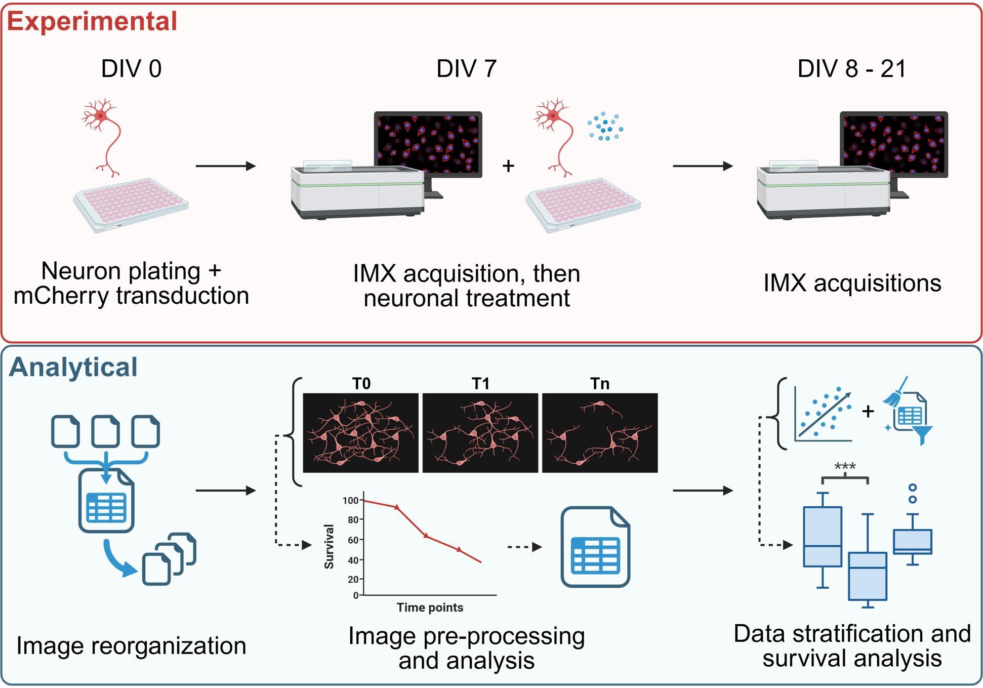
High content survival assay of cortical murine primary neurons, allowing data stratification to account for the trophic effects. IMX= ImageXpress®.
Background
Survival assays measure how treatments affect neuronal viability, but primary cultures are challenging because plating variability affects the number of surviving neurons. However, by taking advantage of their low mobility, we report an innovative, high-content, in vitro survival assay that can image and monitor primary neuronal culture over two weeks. By integrating live imaging and stratifying data by the initial neuronal count, the assay overcomes plating-related variability, including trophic effects, as detailed in our recent publication [1].
Most of the current methods used to quantify the survival of primary cultures require the neuronal cultures to be interrupted at the selected time point. For example, to perform an ELISA assay [2] or any immunofluorescence assay, the cells must be fixed. MTT and luciferase assays (the latter for neurons transfected with firefly luciferase reporter) require cell lysis to quantify survival rates [3]. Trypan blue and propidium iodide staining are membrane permeability-based assays that require cell detachment for counting [3].
Analyses that use culture media as the starting material, such as the quantification of lactate dehydrogenase (LDH) released [3], do not require cell cultures to be lysed or fixed; however, they are unable to account for disparities induced by plating variability and the relative neuronal trophic effect.
A neuronal survival assay in primary neuronal culture, utilizing single-cell and real-time imaging resolution, has been previously reported [4]. Similarly, our method relies on live imaging of fluorescently transduced neurons, enabling the comparison of different time points within the same neuronal culture. Additionally, it is combined with post-acquisition data stratification based on the initial cell number.
Although our novel method has clear advantages over previously published survival assays, some technical limitations are present. First, neuronal primary cultures are sensitive to temperature and CO2 changes induced by plate relocation during the incubator-microscope shift, so this must be considered. For this reason, daily acquisitions over a long period (more than five days) are not recommended. Additionally, technical difficulties may arise when attempting to minimize the shift of the field of view (FOV) during acquisitions at different time points. The position of the plate inside the ImageXpress is crucial, and re-aligning the FOV with the previous ones may take time. Furthermore, the analysis parameters (both in image preprocessing, processing, and post-analysis stratification) must be set up depending on the conditions used for the experiment (e.g., the type of cell used, the selected cell treatment, etc.). In conclusion, it is essential to emphasize that the overexpression of fluorescent reporter proteins through lentiviral transduction results in a slight increase in cell mortality compared to non-transduced controls.
Our survival assay was specifically designed for primary murine cortical neurons, but it can be applied to other primary neuronal cultures or to any other cell culture in which cells have low migration and have exited the cell cycle, such as post-mitotic cells. Through this protocol, neuronal survival curves can be calculated at specific selected time points, allowing several analytical approaches; the conditions of interest, such as enhancement or suppression of biological pathways through drug treatment or genetic modifications, can be followed intra-condition during all time points, or be compared inter-condition with the relative controls at each specific time point.
As previously reported, the aim of this protocol is to conduct a quantitative analysis of neuronal survival with or without specific treatments. The first step involves producing lentiviral particles to induce expression of the fluorescent reporter protein in neurons. Once the viral particles have been isolated from HEK293T cells and quantified, the murine cortical neurons can be plated and transduced. After seven days in culture, the first live imaging acquisition is performed, and the neurons are treated as desired. Additional acquisitions will be performed at different time points (three to five additional time points are recommended). All the images are then reorganized, preprocessed, and analyzed using a semi-automatic Fiji macro pipeline, resulting in a CSV table containing the neuronal count and relative survival rate for each field of view at each time point. Starting from the treatment control, the neuronal trophic effect can then be established, and specific data stratification can be applied to rule out its influence on the survival rate. Once the stratification is optimized, quantitative comparisons of interest can be performed.
To design the experiment properly, it is essential to define the number of conditions to be compared, identify the necessary controls, and determine the number of technical and biological replicates required. Once all of these are acknowledged, the number of wells (and so the number of plates) that are necessary for the experiment can be calculated, as well as the relative quantity of lentiviral particles needed for the transduction. During neuronal plating, it is essential to avoid cellular overconfluency; therefore, we suggest plating 15,000 cells/well in a 96-well plate.
Materials and reagents
Biological materials
Plasmids
1. psPAX2 (Addgene #12260): plasmid containing gag, pol, and rev genes
2. pMD2.G (Addgene #12259): plasmid containing VSV-G envelope gene
3. LentiLox 3.7 syn-mCherry: mCherry sequence under the control of the neuron-specific synapsin I promoter was cloned into a LentiLox 3.7 vector [5]; this newly generated plasmid is available upon request
Cell lines
1. Murine primary cortical neuronal cultures [obtained from embryos (E15.5) derived from wild-type C57BL/6N mice (Charles River Laboratories, ITALIA)]
2. HEK293T cells [American Type Culture Collection (ATCC), catalog number: CRL-3216, origin: human epithelial-like cells isolated from the kidney]
Primers
1. Forward primer: TCCTGCTCAACTTCCTGTCGAG
2. Reverse primer: CACAGGTCAAACCTCCTAGGAATG
Note: 100 μM desalted primers can be purchased from any company that provides this service (e.g., Eurofins, Macrogen).
Reagents
Murine primary cortical neuronal cultures
1. Minimum essential medium (MEM), GlutaMAXTM supplement (Life Tech., catalog number: 41090-028)
2. Fetal bovine serum (FBS) (Gibco, catalog number: 10270-106)
3. Neurobasal (Life Tech., catalog number: 21103-049)
4. Sodium pyruvate (Invitrogen, catalog number: 11360-039)
5. Cytosine arabinoside (AraC) (100 mM) (Merck, catalog number: C1768)
6. Penicillin-streptomycin (PenStrep) (Gibco, catalog number: 15140-122)
7. B27 (50×) (Gibco, catalog number: 17504-044)
8. Poly-D-lysine (Merck, catalog number: P7280)
9. Papain (Merck, catalog number: P4762)
10. Sodium acetate (Merck, catalog number: 241245)
11. DNase I (Merck, catalog number: D5025)
12. L-Cystine (Merck, catalog number: C7602)
13. 1 M hydrochloric acid (HCl) (Merck, catalog number: H9892)
14. Earle’s balanced salt solution (EBSS) (10×) (Merck, catalog number: E7510)
15. Sodium bicarbonate (Merck, catalog number: S5761)
16. Trypsin inhibitor (Merck, catalog number: T9253)
17. Bovine serum albumin (Merck, catalog number: A7030)
18. Ethylenediaminetetra acetic acid (EDTA) (Invitrogen, catalog number: 15575-038)
19. L-Glutamine (Gibco, catalog number: 25030-081)
20. 0.22 μm filters (Euroclone, catalog number: EPSPV2230)
HEK293T cultures and lentiviral particles production and quantification
1. Dulbecco’s modified Eagle medium (DMEM) 1× (Gibco, catalog number: 11960-044)
2. Fetal bovine serum (FBS) (Gibco, catalog number: 10270-106)
3. Penicillin-streptomycin (PenStrep) (Gibco, catalog number: 15140-122)
4. L-Glutamine (Gibco, catalog number: 25030-081)
5. Sodium chloride (NaCl) (Merck, catalog number: S9888)
6. HEPES (N-2-hydroxyethylpiperazine-N’-2-ethanesulfonic acid), 0.5 M buffer solution, pH 7.0 (Thermo Fisher Scientific, catalog number: J60064.AE)
7. Disodium phosphate (Na2HPO4) (Merck, catalog number: S9763)
8. Calcium chloride (CaCl2) (Merck, catalog number: C5670)
9. 0.22 μm filters (Euroclone, catalog number: EPSPV2230)
10. Triton X-100 (Merck, catalog number: T8532)
11. Potassium chloride (KCl) (Merck, catalog number: P3911)
12. Tris base (Merck, catalog number: T6687)
13. Glycerol (Merck, catalog number: G5516)
14. Ribolock RNase inhibitor (Thermo Fisher Scientific, catalog number: EO0381)
15. Ammonium sulfate [(NH4)2SO4] (Merck, catalog number: A4915)
16. Magnesium chloride (MgCl2) (Thermo Fisher Scientific, catalog number: R0971)
17. BSA (NEB, catalog number: B9000)
18. SYBR Green I (Thermo Fisher Scientific, catalog number: S7563)
19. Tris-EDTA (TE) buffer solution, pH 8.0, RNase-free (Invitrogen, catalog number: AM9849)
20. dNTPs (Thermo Fisher Scientific, catalog number: R0191)
21. MS2 RNA (Roche, catalog number: 10165948001)
22. DreamTaq Hot Start DNA Polymerase (Thermo Fisher Scientific, catalog number: EP1701)
Additional materials
1. Ethanol (Merck, catalog number: 459844)
2. PhenoPlate 96-well (PerkinElmer, catalog number: 6055300)
Solutions
1. Sodium acetate solution pH 4.5 (50 mM) (see Recipes)
2. Papain stock solution (see Recipes)
3. DNase I stock solution (see Recipes)
4. L-Cystine stock solution (see Recipes)
5. 1× EBSS solution (see Recipes)
6. 10/10 solution (see Recipes)
7. Papain solution (see Recipes)
8. EBSS-10/10 solution (see Recipes)
9. Plating media (see Recipes)
10. Neurobasal complete (see Recipes)
11. 1× Poly-D-lysine solution (0.01 mg/mL) (see Recipes)
12. DMEM complete (see Recipes)
13. NaCl stock solution (5 M) (see Recipes)
14. Na2HPO4 stock solution (0.15 M) (see Recipes)
15. 2× HPB (see Recipes)
16. CaCl2 stock solution (2.5 M) (see Recipes)
17. KCl stock solution (5 M) (see Recipes)
18. Tris-HCl pH 7.4 (1 M) and pH 8.3 (2 M) (see Recipes)
19. 2× lysis buffer (see Recipes)
20. (NH4)2SO4 stock solution (500 mM) (see Recipes)
21. 10× core buffer (see Recipes)
22. MgCl2 stock solution (25 mM) (see Recipes)
23. SYBR Green I stock solution (see Recipes)
24. MS2 RNA stock solution (see Recipes)
25. 2× reaction buffer (see Recipes)
Recipes
1. Sodium acetate solution pH 4.5 (50 mM)
Prepare an aqueous solution of sodium acetate and adjust it to the appropriate pH with a solution of HCl. Prepare the solution fresh and keep it at room temperature (RT) before use.
2. Papain stock solution
Dissolve lyophilized papain powder in 50 mM sodium acetate, pH 4.5 (prepared from the stock solution), to a stock concentration of 100 units/mL. Store at 4 °C for up to 6 months.
3. DNase I stock solution
Dissolve lyophilized DNase I powder in sterile water to prepare a stock solution of 1 mg/mL. Store at -20 °C for up to 6 months.
4. L-Cystine stock solution
Dissolve L-Cystine in 1 M HCl to prepare a stock solution of 100 mM. Store at 4 °C for up to 6 months.
5. 1× EBSS solution (for 500 mL)
Add 50 mL of 10× EBSS and 1.1 g of sodium bicarbonate. Adjust the volume with double-distilled water and filter-sterilize. Store at 4 °C for up to 1 month.
6. 10/10 solution (for 50 mL)
Add 500 mg of trypsin inhibitor and 500 mg of bovine serum albumin (Merck, A7030) and adjust the volume with 1× EBSS solution. Filter-sterilize and store at 4 °C for up to 1 month.
7. Papain solution (for 30 mL)
Add 200 μL of papain stock solution, 30 μL of EDTA, and 30 μL of cysteine stock solution (100 mM). Adjust the volume with 1× EBSS solution and filter-sterilize. Prepare fresh and keep at 37 °C before use.
8. EBSS-10/10 solution
Add 4.5 mL of 1× EBSS solution and 0.5 mL of 10/10 solution. Prepare fresh and keep at 37 °C before use.
9. Plating media (for 50 mL)
Add 5 mL of FBS and 0.5 mL of PenStrep and adjust the volume with MEM, GlutaMAXTM supplement. Prepare fresh and keep at 37 °C before use.
10. Neurobasal complete (for 50 mL)
Add 0.5 mL of sodium pyruvate, 1 mL of B27 (50×), 0.5 mL of PenStrep, 0.5 mL of L-Glutamine, and 50 μL of Ara C (100 mM). Adjust the volume with neurobasal medium. Prepare fresh and keep at 37 °C before use.
11. 1× Poly-D-lysine solution (0.01 mg/mL)
Dilute the 1 mg/mL Poly-D-lysine stock solution 1:100 in PBS 1×. Prepare fresh and keep at RT before use.
12. DMEM complete
Supplement DMEM 1× with 10% FBS, 1% PenStrep, and 1% L-Glutamine. Store at 4 °C for up to 1 month.
13. NaCl stock solution (5 M)
Prepare an aqueous solution of NaCl at the appropriate concentration. Store at RT for up to 6 months.
14. Na2HPO4 stock solution (0.15 M)
Prepare an aqueous solution of Na2HPO4 at the appropriate concentration. Store at RT for up to 6 months.
15. 2× HPB (for 100 mL)
Add 0.28 M NaCl (5.6 mL of 5 M NaCl stock solution), 0.05 M HEPES pH 7.0, and 0.0015 M Na2HPO4 (1 mL of 0.15 M Na2HPO4 stock solution). Adjust pH to 7.1 with NaOH. Adjust the volume with double-distilled water. Filter-sterilize and store at 4 °C for up to 6 months.
16. CaCl2 stock solution (2.5 M)
Prepare an aqueous solution of CaCl2 at the appropriate concentration. Filter-sterilize and store at 4 °C for up to 6 months.
17. KCl stock solution (5 M)
Prepare an aqueous solution of KCl at the appropriate concentration. Store at RT for up to 6 months.
18. Tris-HCl pH 7.4 (1 M) and pH 8.3 (2 M)
Prepare an aqueous solution of Tris base and adjust it to the appropriate pH with a solution of HCl. Store at RT for up to 6 months.
19. 2× lysis buffer
Add 0.25% Triton X-100, 50 mM KCl (from stock solution), 100 mM Tris-HCl, pH 7.4 (from stock solution), 40% glycerol, and 0.8 U/μL Ribolock RNase inhibitor. This buffer can be stored at RT for up to 6 months without RNase inhibitor. Prepare a freshly aliquoted complete buffer from the incomplete one and add the appropriate amount of RNase inhibitor just before viral particle lysis.
20. (NH4)2SO4 stock solution (500 mM)
Prepare an aqueous solution of (NH4)2SO4 at the appropriate concentration. Store at RT for up to 6 months.
21. 10× core buffer
Add 50 mM (NH4)2SO4 (from stock solution), 200 mM KCl (from stock solution), and 200 mM Tris-HCl, pH 8.3 (from stock solution). Adjust the volume with double-distilled water. Store at RT for up to 6 months.
22. MgCl2 stock solution (25 mM)
Prepare an aqueous solution of MgCl2 at the appropriate concentration. Store at RT for up to 6 months.
23. SYBR Green I stock solution
Dilute the original SYBR Green I stock 1:100 in TE buffer solution, pH 8.0, RNase-free. Aliquot (20 μL) and store at -80 °C for up to 6 months. Once thawed, do not reuse.
24. MS2 RNA stock solution
The original MS2 RNA stock is 0.8 μg/µL, i.e., 0.7 pmol/µL. Aliquot (15 μL) and store at -80 °C for up to 6 months.
25. 2× reaction buffer
Add 5 mM (NH4)2SO4, 20 mM KCl, 20 mM Tris-HCl (pH 8.3), 10 mM MgCl2, 0.2 mg/mL BSA, 1:10,000 SYBR Green I, 400 μM dNTPs, 1 μM forward primer, 1 μM reverse primer, 7 pmol/mL MS2 RNA, and 20 U of RNase inhibitors. Prepare using a 10× core buffer according to the table below and store in 50 μL aliquots at -80 °C for up to 6 months.
| Compound | Stock | 2 reactions (μL) | 100 reactions (μL) | 300 reactions (μL) |
|---|---|---|---|---|
| 10× core buffer | Stock solution | 1 | 50 | 150 |
| MgCl2 25 mM | Stock solution | 4 | 200 | 600 |
| 100× BSA | NEB, B9000 | 0.2 | 10 | 30 |
| dNTPs 10 mM | Thermo Fisher Scientific, R0191 | 0.4 | 20 | 60 |
| Primer fwd 100 μM | Stock solution | 0.1 | 5 | 15 |
| Primer rev 100 μM | Stock solution | 0.1 | 5 | 15 |
| MS2 RNA | Roche, 10165948001 | 0.1 | 5 | 15 |
| SYBR Green I 1:100 | Stock solution | 0.1 | 5 | 15 |
| H2O | 4 | 200 | 600 | |
| RNase inhibitor | Thermo Fisher Scientific, EO0381 | 0.01 | 0.5 | 1.5 |
Equipment
1. ImageXpress® micro confocal high-content inverted imaging system from Molecular Devices, equipped with:
a. Andor Zyla 4.2 Megapixel sCMOS digital camera
b. Lumencor Spectra light engine LED light source
c. 576/23 nm excitation filter, 624/40 nm emission filter, and 594 nm single-band dichroic mirror
d. Nikon Plan Apo 10×/0.45 dry objective
e. Incubation system with temperature and CO2 control
2. Tabletop centrifuge (Eppendorf, model: Centrifuge 5804)
3. Touch Real-Time PCR Detection System (Bio-Rad, model: CFX96)
Software and datasets
1. MetaXpress from Molecular Devices, for image acquisition (https://it.moleculardevices.com/products/cellular-imaging-systems/high-content-analysis/metaxpress)
2. Python 3.13, for microscopy data organization (https://www.python.org/downloads/)
3. Fiji (Fiji Is Just ImageJ), for image analysis (https://imagej.net/software/fiji/downloads)
4. GraphPad Prism, for data representation (https://www.graphpad.com/features)
Programming languages
1. ImageJ macro language
2. Jython
3. Python3
Procedure
A. Lentiviral particle production and quantification
A1. HEK293T plating and transfection
1. Plate HEK293T cells in 100 mm dishes in 8 mL of complete DMEM at a concentration of 3 million cells/dish.
CRITICAL: Cells should not be too confluent and well dispersed for transfection. Cells in the middle of a clamp will not be transfected.
2. The following day, to perform transfection, bring all the required solutions to RT before starting.
3. In Eppendorf tubes or using a single well of a 24-well tissue culture plate, prepare the following DNA mix for each 100 mm dish:
a. Dispense 450 μL of sterile water (subtract the volume of DNA to be added, if this is significantly high).
b. Add DNA (20 μg) with the following proportion: 7.5 μg of gag-pol (PAX2 vector), 2.5 μg of envelope (VSV-G vector), and 10 μg of viral plasmid of interest (here, syn-mCherry).
c. Add 50 μL of CaCl2 and mix by pipetting up and down.
CRITICAL: High-quality, endotoxin-free DNA improves transfection efficiency.
4. Dispense 500 μL of 2× HPB in another tube/well.
5. Add the DNA mix onto the 2× HPB drop by drop, without mixing.
6. Incubate at RT for 20–25 min. The solution will become cloudy with a slightly milky appearance.
CRITICAL: A longer incubation time will result in larger complexes, which are less effective for transfection.
7. Add the mixture (1 mL) dropwise onto the cell culture dish.
8. Incubate cells for 16 h (overnight if the transfection is performed in the afternoon) in a standard humidified CO2 incubator set to 37 °C and 5% CO2 and replace the medium with 8 mL of fresh DMEM the following day.
A2. Lentiviral particles isolation and quantification
1. After 48 h from transfection, collect the culture media and centrifuge it at 1,200 rcf for 10 min at RT to remove any detached cells.
2. Filter the culture media through a 0.22 μm filter.
CRITICAL: Save a 10 μL aliquot for particle titration. Viral particles can be aliquoted and stored at -80 °C for later use in experiments.
3. Before infection, we recommend quantifying the viruses using the SG-PERT reverse transcription assay [6]. This assay requires a standard curve obtained using known concentrations of high-titer viral supernatants (we suggest using 107, 106, 105, and 104 pU standards). To perform the SG-PERT reverse transcription assay, proceed as follows:
a. Prepare the lysis buffer (e.g., 10 μL for each sample) by adding 2 μL of RNAse inhibitor to every 100 μL of 2× lysis buffer.
b. Under the biological hood, aliquot 10 μL of 2× lysis buffer in 1.5 mL Eppendorf tubes and mix with 10 μL of virus suspension (from both your samples and the standards, if needed).
c. Incubate at RT for 10 min (after this time, the virus is not infectious anymore, and you can work on the bench).
d. Prepare 1× core buffer by diluting the 10× core buffer in water (Milli-Q or autoclaved).
e. Dilute the lysed virus (both your samples and the standards) 1:10 in 1× core buffer (e.g., 2 μL of virus/standard + 18 μL of 1× core buffer). Mix well (vortex if convenient).
f. Thaw the required amount of 2× reaction buffer (5 μL for each sample and standard) and add Hot Start Taq DNA polymerase (5 units in 100 μL of 2× reaction buffer = 1 μL in 100 μL of 2× reaction buffer). Mix and aliquot 5 μL into the wells of an RT-PCR plate.
g. Add 5 μL of diluted samples (your samples and standards) to the 2× reaction buffer in the RT-PCR plate and mix (10 μL total volume for the PCR). Avoid the formation of bubbles.
h. Seal the plate and briefly spin it.
i. Load the cycler and start the RT-PCR reaction. The RT-PCR program (using Bio-Rad CFX96) is as follows: 42 °C for 20 min for RT reaction, 95 °C for 2 min for enzyme activation, followed by 40 cycles of denaturation at 95 °C for 5 s, annealing at 60 °C for 5 s, extension at 72 °C for 15 s, and acquisition at 80 °C for 7 s. Melting curve: 65 °C, 5 s + 0.5 °C/cycle, ramp 0.5 °C/s.
CRITICAL: Caution must be exercised when producing and handling lentivirus. Familiarize yourself with the potential hazard and the necessary precautions. Always wear PPE and decontaminate potentially infectious waste before disposal. Aliquoting viral particles to reduce the number of freeze-thaw cycles is strongly recommended. We suggest using aliquots of virus concentrated enough so that the required volume does not exceed 1/10 of the total volume of the transduced well. The viruses and standards can be stored in lysis buffer at -80 °C. Instead, once diluted in 1× core buffer, they cannot be stored (after 5–6 h, they lose reverse transcriptase activity). It is necessary to dilute the virus at least 10 times in 1× core buffer; however, it is also possible to further dilute it. There is no problem if you create bubbles while diluting the virus. Avoid creating bubbles when loading the reaction buffer and diluted virus into the RT-PCR plate. During the RT-PCR protocol, we acquire the fluorescence signal at 80 °C to avoid the signal that may derive from primer dimers or nonspecific sequences.
4. Starting from the output file generated from the Bio-Rad CFX96 Touch Real-Time PCR Detection System, identify the cycle threshold (Cq) values of all the samples processed, including the standards, and proceed as follows (Figure 1):
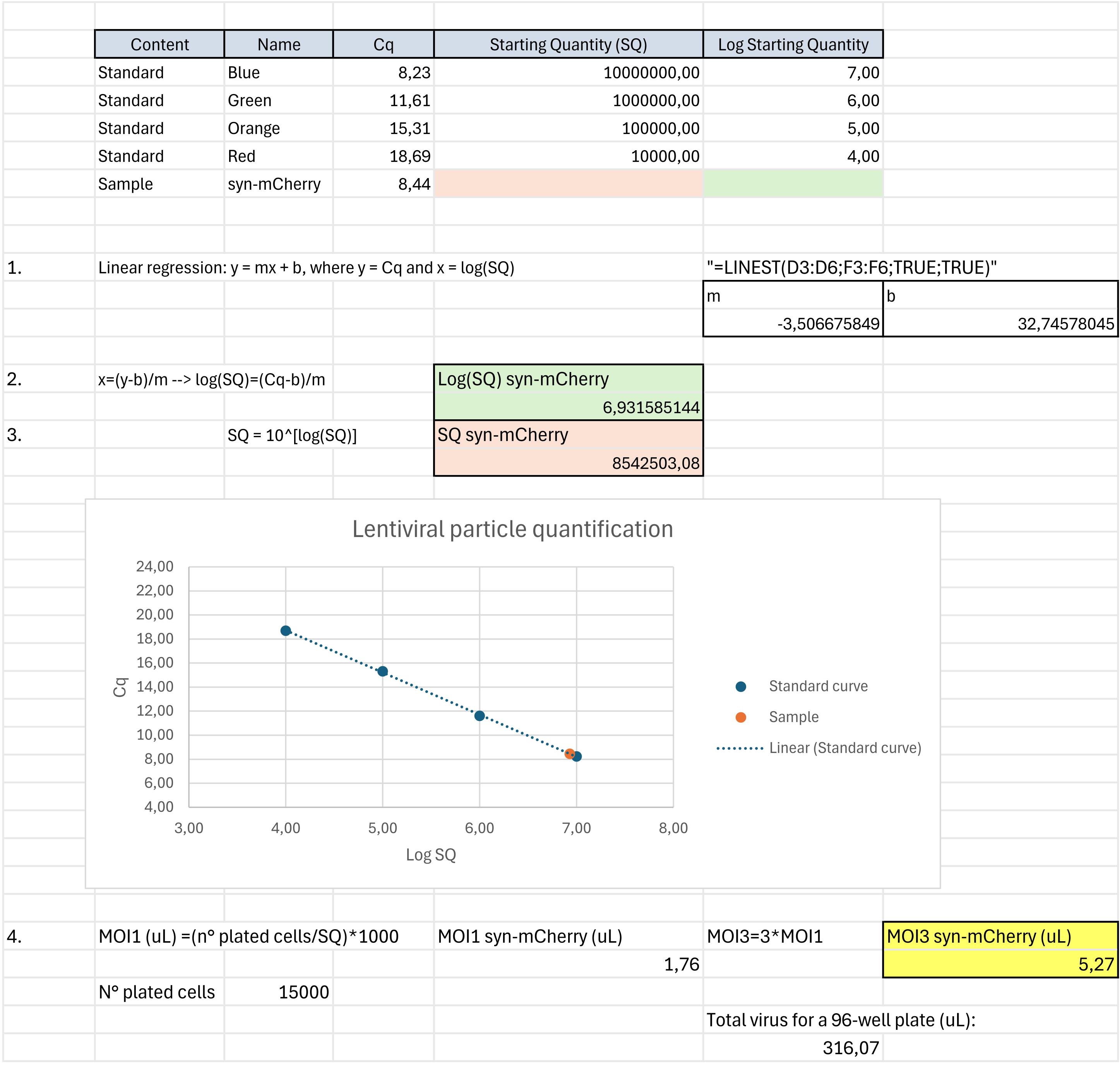
Figure 1. Lentiviral particle quantification. Example of the procedure to calculate the titer of the lentiviral particles produced and the volume for the multiplicity of infection (MOI) necessary for transduction. The procedure was divided into four main steps: linear regression for the standard curve (1), calculation of the logarithm of the starting quantity (2), calculation of the starting quantity (3), and calculation of the required volume of viral particles per well (4).
a. Create a table with Cq, starting quantity (SQ), and log(SQ) for all your standards.
b. Calculate the linear regression for your standards to obtain the standard curve, as reported in Figure 1 (1.).
c. Starting from the Cq value of your sample (e.g., syn-mCherry), calculate the log(SQ) and the SQ, as reported in Figure 1 (2. and 3.).
d. Once the SQ of the desired sample (e.g., syn-mCherry) is obtained, calculate the volume of viral particles per well to obtain a multiplicity of infection (MOI) of 3, as reported in Figure 1 (4.).
CRITICAL: As long as the viral particle concentration of the sample produced is similar to the one reported in Figure 1 (just below 107 pU), small volumes (around 5 μL) are required to reach a MOI of 3 for wells with 15,000 cells/well, meaning that around 300 μL are sufficient to transduce a whole (60 wells) 96-well plate. The average volume of viral particles produced from a 100 mm dish is approximately 7–7.5 mL after collection and filtration, which allows for the transduction of approximately twenty 96-well plates.
B. Preparation of murine primary cortical neurons
1. The day before the dissection (or at least 2 h before), coat 96-well plates with 50 μL of 1× poly-D-lysine solution and incubate at 37 °C.
CRITICAL: To minimize experimental variability, we strongly recommend avoiding the peripheral wells of the 96-well plate, as they are more susceptible to external stimuli, such as temperature and humidity changes, which can affect neuronal survival. For these reasons, we suggest adding 200 μL of PBS 1× to the peripheral wells (to maintain humidity more effectively) and plating the neurons in the remaining 60 wells. Additionally, since the bottom of the plate is quite delicate, we suggest keeping the plates on top of an extra 96-well plate lid to prevent scratches on the surface while moving them in the incubator.
2. Before starting the dissection, prepare the following solutions fresh and incubate them at 37 °C: papain solution (30 mL), EBSS-10/10 (5 mL), and neurobasal complete.
3. In addition, prewarm at 37 °C the 10/10 solution (5 mL) and the plating media.
CRITICAL: Volumes reported in steps B2–3 are suitable for experiments with cortices derived from 6–7 embryos. If more cortices are processed simultaneously, please adjust the volumes proportionally. If cortices from each mouse need to be processed separately (single embryo), prepare the following for each: 5 mL of papain solution, 0.5 mL of EBSS-10/10, and 0.5 mL of 10/10 solution.
4. Dissect the cortices with sterilized surgical instruments in 70% EtOH, placing the entire dissection in a 100 mm dish containing ice-cold 1× PBS.
5. Filter the papain solution and transfer the cortices into the papain (30 mL for the mix or 5 mL each for single embryos). Incubate in a 37 °C water bath for 20 min, swirling gently every 3 min (cortices will appear mushy or loose toward the end of the incubation).
6. Continue to dissociate the cortices by gently pipetting up and down with a 10 mL serological pipette (no more than 10 up and down movements along the side of the tube in slow pipette mode).
7. Add 100 μL (or 16.7 μL for a single embryo) of DNase I (1 mg/mL) to the resuspension, mix gently by pipetting up and down with a 10 mL pipette, and incubate at 37 °C for an additional 3 min.
8. Centrifuge at 1,000 rcf in a tabletop Eppendorf centrifuge for 5 min at RT.
9. Remove the supernatant and add 5 mL (0.5 mL for a single embryo) of EBSS-10/10 solution. Resuspend the pellet by pipetting up and down, and then transfer the suspension to a 15 mL Eppendorf tube. Add 5 mL (0.5 mL for a single embryo) of the 10/10 solution gently alongside the tube wall, avoiding mixing or shaking the solution.
10. Centrifuge at 1,000 rcf in a tabletop Eppendorf centrifuge for 10 min at RT.
11. During centrifugation, aspirate the poly-D-lysine coating from the wells.
12. Drain off the supernatant, resuspend the pellet in 10 mL (1 mL for a single embryo) of plating media, and count the cells. Plate 15,000 cells/well in 100 μL of plating media. Plating day is counted as day 0.
CRITICAL: From two cortices of a single pup, the average number of cells derived is approximately 7–9 million neurons. Since a 96-well plate has 60 available wells suited for neuronal culture, as described above, the total number of neurons required for seeding is 900,000 cells, a number well covered by a single pup.
C. Transduction of cortical neurons with lentiviral particles
1. Around 4 h after plating, transduce neurons with lentiviral particles with a MOI of 3 to induce the expression of syn-mCherry fluorescent protein.
CRITICAL: Due to the presence of the synapsin promoter, mCherry will be translated only in neuronal cells. We recommend using concentrated lentiviral particles (maximum 10 μL/well) to minimize additional toxicity due to the excessive presence of “non-neuronal plating” media.
2. The day after (day 1), change the whole media with neurobasal complete.
3. Leave in the incubator for 6 days (day 7) for the first image acquisition.
CRITICAL: Fluorescence should be visible by around day 4 or 5. For reference, the average transduction efficiency achieved with a MOI of 3 is approximately 15%–30% mCherry-positive neurons on day 7. While higher MOI values can increase transduction yield, they also increase neuronal death. Therefore, caution must be exercised when deciding whether to increase the MOI value.
D. Image acquisition
1. Approximately 30 min before acquisition, turn on the incubation system of the ImageXpress®, setting the conditions required for live-cell imaging (37 °C and 5% CO2).
2. Select a low magnification objective (in our case, a Plan Apo 10×/0.45 dry objective).
3. Transfer the plate with the cell cultures as quickly as possible, directly from the cell incubator to the imaging system. Before inserting the plate, clean the bottom of each 96-well plate with 70% ethanol.
CRITICAL: Please note that primary neurons are highly sensitive to changes in temperature and CO2. Therefore, we recommend minimizing the transfer time from the cell incubator to the imaging system to 1–3 min, if possible, and avoiding light exposure. If the plate is kept outside any incubation system for more than 5 min, survival could be affected.
4. In the imaging system, place the plate firmly against the same corner of the chamber each time (e.g., top-right). Record this position.
5. Set the acquisition parameters for single-channel image acquisition. In our case, the acquisition parameters to detect cellular mCherry signal were set as follows:
576/23 nm excitation filter, 624/40 nm emission filter, and 594 nm single-band dichroic mirror.
Camera binning 1 × 1, pixel size 0.6728 μm × 0.6728 μm.
100 ms exposure time.
100% illumination power.
MetaXpress “FL Shading only” shading correction.
Single widefield image, no Z-stack.
Autofocus “focus on plate and well bottom” active: standard algorithm with binning 2.
CRITICAL: Acquisition parameters must be optimized according to the observed fluorescent signal. It is essential to minimize both the duration and intensity of illumination to prevent signal bleaching and phototoxicity, as the procedure involves live-cell imaging.
6. Select five fields of view (FOVs) per well and proceed with the acquisitions.
7. The acquisition of the same FOVs will be repeated at precise time intervals (time points), repeating the procedure described above (steps D1–6).
8. Name the acquisition files following these specific guidelines. As later discussed, a script will automatically move the files to the correct folders. To do so, it checks for the following pattern in the filename:
.*-[tT](?P<T>\d+)_(?P<W>[A-Z]\d+)_[sS](?P<S>\d+)
Which corresponds to matching all the strings that have a format similar to:
<anything>-T<number>_<any_upper_case_letter><number>_S<number>
<anything>-t<number>_<any_upper_case_letter><number>_s<number>
For example:
96w-10Xpa-Neural-Tox-P2A-T0_B02_s1.tif
It is fundamental that the part regarding the time points (underlined), the well (in bold), and the field of view within the well (in italics) are together as shown above.
CRITICAL: Caution must be exercised when naming the file, as it will be relevant to the data reorganization for the subsequent analysis.
9. After image acquisition, bring the plate back into the incubator (as quickly as possible).
E. Cell treatment
Following the initial acquisition (T0), cellular treatment can be performed if desired. Several approaches can be used, such as drug or biomolecule treatments, or any other treatment whose biological effect is to be determined. We recommend using proper controls:
1. Treatment control: In cases of treatments with drugs or biomolecules, include control wells where the same addition of media (type and volume) is performed without the small molecule or biological compound.
2. Death control: Include control wells where the media is substituted with media without the B27 supplement to induce neuronal death and have a death control.
CRITICAL: Controls are essential for the correct interpretation of the data. We suggest replicating a specific condition in at least five wells to ensure enough technical replicates. Assuming four conditions of interest to compare, half of a plate should be enough for each biological replicate. Here, we report a practical example of a plate (Figure 2): dividing the plate into two halves, one for each biological replicate, the first row (B) will be dedicated to the death control, while the second (C) to the treatment control. Rows from D to G will be dedicated to conditions of interest. We recommend performing at least three biological replicates. Using pools of animals instead of a single animal as a biological replicate will strengthen the reliability of the obtained data.
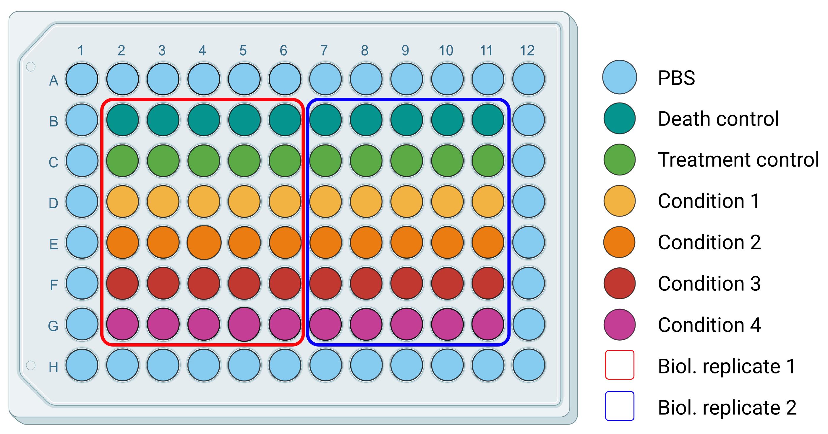
Figure 2. Plating organization for survival assay. Example of a 96-well plate organization, differentiating conditions for technical and biological replicates.
F. Acquisitions after treatment
CRITICAL: Following acquisition, dates can be adapted to the necessities dictated by specific treatments, requiring, for example, earlier or later time points. However, we suggest 3–5 time points in total. Moreover, primary neurons are highly sensitive to temperature and CO2 changes; therefore, we discourage daily acquisitions, as their survival will be affected.
1. Approximately 30 min before acquisition, turn on the incubation system of the ImageXpress®, setting the conditions required for live-cell imaging (37 °C and 5% CO2).
2. In the imaging system, select the same objective used for day 1 acquisition (in our case, the Plan Apo 10×/0.45 dry objective).
3. Transfer the plate with the cell cultures directly from the incubator to the imaging system. Gently push the plate against the same corner of the chamber, selected at passage D4. Before inserting the plate, clean the bottom of each 96-well plate with 70% ethanol.
CRITICAL: For each acquisition after treatment, it is essential to reposition the plate in the exact location where it was on the day of the first acquisition to minimize cellular shift between acquisitions (as shown in Figure 3). Larger shifts may affect the neurons visualized within the FOV, resulting in the loss of previously acquired cells or the addition of neighboring cells. This, of course, will affect the biological results since the observed cohort will not be consistent over time. To achieve this, we suggest checking the spatial coordinates of a few FOVs:
a. Starting, for example, from a well in the top-left corner of the plate, perform an acquisition of that FOV and then open the corresponding image previously acquired at time point 0 on the ImageXpress®.
b. Select as a reference the signal of one or more specific neurons, measure their distance in X and Y from the edges in both images, and calculate the respective differences.
c. Adjust the position of the plate by the length differences in X and Y with the ImageXpress® controls, so that the locations of the neurons of reference correspond.
d. Now, check if the correspondence of the FOVs is also relevant in wells located in different areas of the plate (e.g., bottom-right, top-right corner, etc.).
e. If you encounter difficulties repositioning the plate, we suggest removing and reinserting it into the imaging system, paying attention to properly push the plate against the corner selected at passage D4, and then repeating passaged a-d.
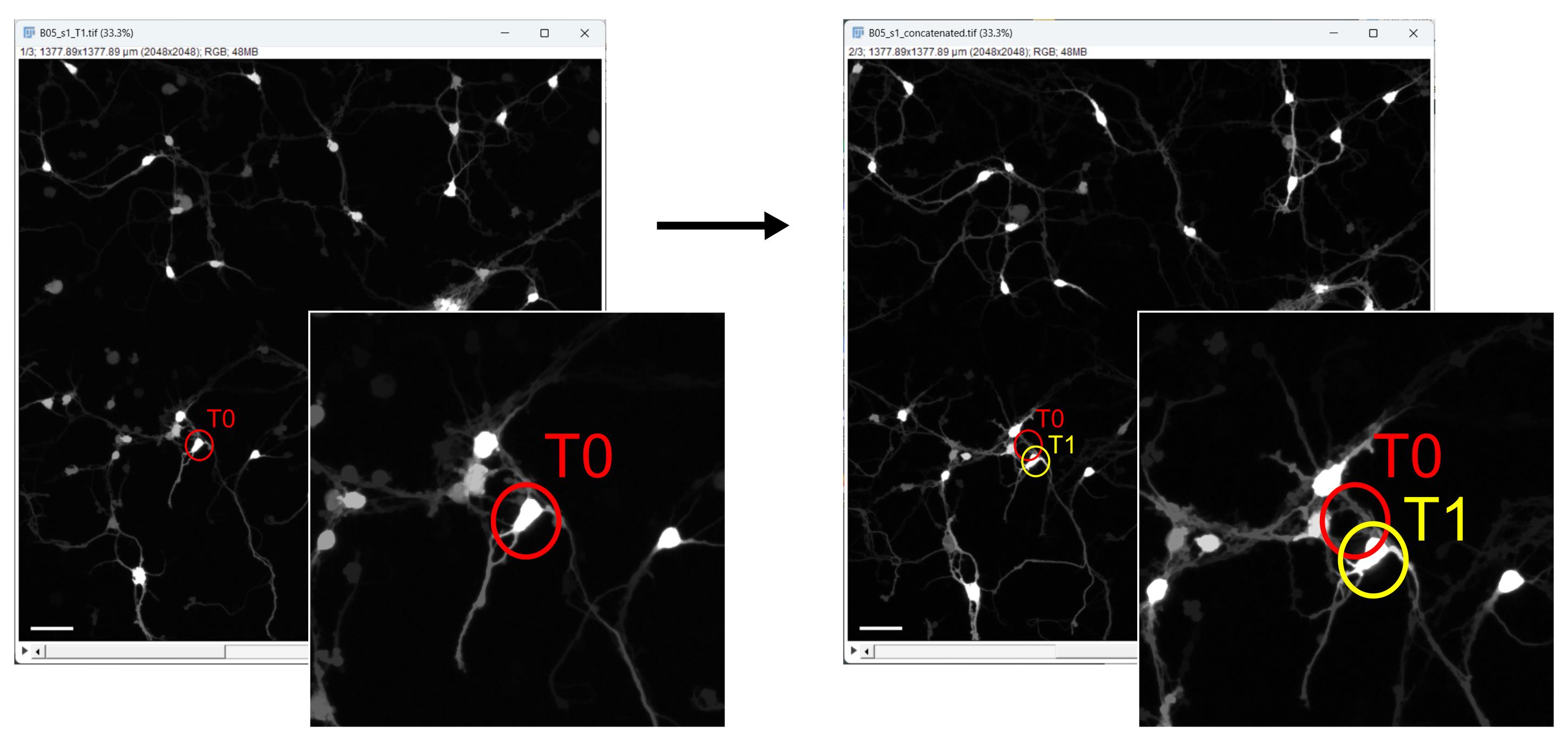
Figure 3. Plate positioning and cellular shift evaluation after the first acquisition . Example of a small cellular shift in the field of view, comparing the position of a selected neuron at time point 0 (T0) in red and time point 1 (T1) in yellow. Scale bar, 100 µm.
4. Proceed with the acquisitions as previously reported in steps D5–6.
5. When naming the acquisition files, please keep in mind all the requirements outlined in passage D8.
G. Python installation and configuration
CRITICAL: To proceed to image reorganization and analysis, it is necessary to download all the necessary programs, scripts, and macros. We have uploaded all the material associated with this paper onto our GitHub repository (https://github.com/icosac/High-content-in-vitro-survival-assay-of-cortical-neurons/). Along with all the required materials, we have provided a detailed description of how to download the required programs and how the scripts and macros work. For convenience, we outline the procedure step by step throughout the entire article.
1. Python 3.13 installation procedure (Windows)
a. Access the official Downloads section of the Python website (https://www.python.org/downloads/). From the list, select the 3.13 version and click on Download.
b. In the Python 3.13 download page, scroll to the list of available files and click on the Windows installer (executable file).
c. Scroll further to locate the Download installer (MSIX) button and download it.
d. Locate the downloaded MSIX file (e.g., “python-manager-25.1.msix”) in your download directory and double-click the file to launch the installation manager. If a security warning pops up regarding the execution of an executable file, confirm to proceed.
e. In the Installation Manager, click the Install button to initiate the installation process. If Reinstall is shown instead, Python is already installed on your computer. You can reinstall it to ensure you have the correct version, but be warned that reinstallation will overwrite the existing installation and may alter settings.
f. If a shell window opens requesting permission to change global settings:
i. Press the Y key on your keyboard and then press the Enter key to continue.
ii. Approve the Windows dialog requesting permission for the Python install manager to make changes to your device. Click Yes to continue.
g. If prompted to configure the global shortcuts directory, press the Y key and then press Enter to continue.
h. If informed that a newer Python version is available, press the N key and then press Enter to retain the current version (3.13).
i. If asked whether to view the online help, press the N key and then press Enter to finish the installation. If you want to view the help, press the Y key instead.
2. Python 3.13 installation procedure (MacOS)
MacOS usually comes with Python pre-installed.
3. Python 3.13 installation procedure (Ubuntu)
a. Open a terminal window.
b. Update the package list by running the following command: “sudo apt update”.
c. Install the required dependencies by running the following command: “sudo apt install -y software-properties-common”.
d. Add the deadsnakes PPA (Personal Package Archive) to your system by running the following command: “sudo add-apt-repository ppa:deadsnakes/ppa”.
e. Update the package list again by running the following command: “sudo apt update”.
f. Install Python 3.13 by running the following command: “sudo apt install-y python3.13”.
H. File and folder structure for analysis pipeline execution
CRITICAL: The acquired image files, as they are saved by the acquisition system, are initially divided into folders organized by time and plate, with subfolders organized by time points. This structure is highly inefficient for the final processing of the data, while also storing important information in the folder’s name. For this reason, a script, namely “reorder_starting_from_tx.py,” is used to move the images into a new and more appropriate structure (Figure 4).
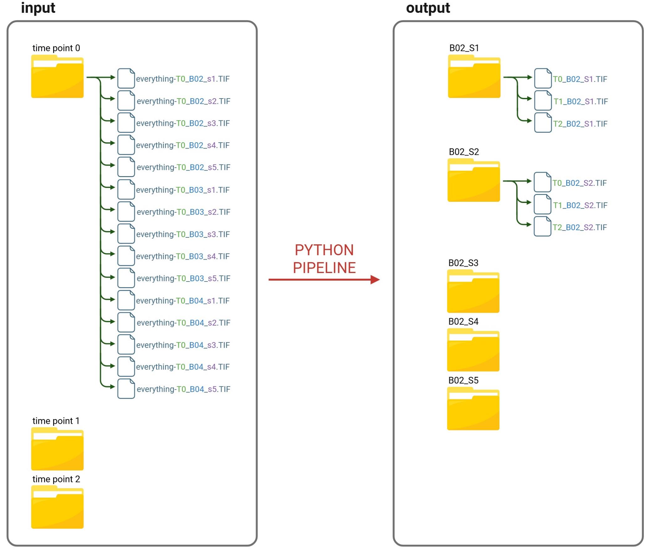
Figure 4. Python pipeline “reorder_starting_from_tx.py” overview. Visual representation of the Python pipeline reordering files for automated image analysis. The script organizes the acquired image files to enable the execution of subsequent analysis pipelines. In particular, it reorganizes the files from time point–based folders in the input directory into field of view (FOV)-based folders in the output directory.
To run this script, put the script inside the main folder containing all the images to be reordered. It will then reorganize files from time point–based folders in the input directory into FOV-based folders in the output directory, as shown in Figure 4.
On Windows: Navigate to the folder where the script is located, then right-click in the folder and choose Open in Terminal from the context menu. In the terminal window that opens, run the following command: “python3 reorder_starting_from_tx.py”. It should terminate without errors.
On macOS or Linux: Open a terminal window, navigate to the folder where the script is located using the cd command, and run the following command: “python3 reorder_starting_from_tx.py”.
The script works as follows:
1. It creates a list of all the images inside the main folder.
a. Starting from the initial directory containing all the subfolders, it retrieves the names of all the files and folders within that folder.
b. Checks if the name ends with .TIF or .tif, indicating that it is an image file. If it does, then it is added to a list of files that must be moved.
c. If the file is not a TIF file, then the script checks if the name corresponds to a directory. If it does, then the function restarts from point 1a; otherwise, the file name is skipped completely.
After this function has finished, all filenames that need to be moved have been inserted into a list, which will then be used as input for the second function, described hereafter.
2. It moves all the images into a more appropriate structure.
a. For each image in the list, the script takes the file name.
b. As mentioned in step D8, the script matches the line with this pattern:
.*-[tT](?P<T>\d+)_(?P<W>[A-Z]\d+)_[sS](?P<S>\d+).
c. From this, the script extracts the necessary information regarding the time, the well, and the FOV in the well.
d. These are then used to create folders in the form “well_FOV”, allowing for the reordering of images by well and field of view. For example, for the previous TIF image, the folder B02_S1 will be created if it does not exist.
e. Finally, the images are moved to their corresponding folders, and their names are modified to contain only the necessary information. For instance, the previous example is moved to the folder B02_S1, and its name is changed to T0_B02_S1.TIF.
I. Fiji installation
The software used to analyze the acquired images is the open-source platform Fiji (Fiji Is Just ImageJ), which can be installed from the official Fiji website at Fiji.sc [7].
Fiji is distributed as a portable application, so you do not need to run an installer. Simply download the archive, extract it to a folder of your choice, and run the Fiji executable inside the extracted folder.
CRITICAL: If you are installing Fiji on Windows, it is strongly recommended to place the Fiji installation directory in a location that is not a system drive.app folder within your user directory (e.g., C:\Users\[your name]\Fiji.app) instead of system-wide locations like C:\Program Files. Storing the Fiji.app folder in protected directories may prevent it from updating, as Windows restricts write permissions in those areas.
J. Fiji configuration for image analysis
Before starting the analysis, several Fiji plugins must be installed locally by following the steps below:
1. Open the Fiji updater: Launch Fiji, then select Help > Update... from the menu to open the updater tool.
2. Manage update sites:
If Fiji is already up to date, a dialog box stating “Your ImageJ is up to date!” will appear. Click OK to continue, then select Manage Update Sites in the updater window.
If updates are available, they will be listed in the ImageJ Updater window. In this case, proceed directly by clicking Manage Update Sites in the same window.
In both cases, a dialog window will open, allowing you to enable additional plugin update sites.
3. Activate required update sites: In the list of available update sites, check the following:
a. IJPB-plugins: Required to install the MorphoLibJ plugin [8].
b. CSBDeep [9], TensorFlow [10], and StarDist [11]: Required for deep learning-based segmentation with StarDist.
c. TrackMate-StarDist: Required for the integration of StarDist with the TrackMate plugin.
4. Apply changes. Once the desired update sites have been selected, confirm the selection by clicking Apply and Close to exit the dialog.
5. Download and restart. The Updater will now list plugins from the newly added update sites for installation and updating. Click Apply Changes to install the selected plugins. Once the installation is complete, restart Fiji to finalize the setup.
K. Image analysis
Automation of cell survival analysis was achieved through the development and sequential execution of two custom macros written for Fiji image analysis software, which require appropriate pre-configuration, as outlined in sections I and J.
The first macro, named “survival_preprocess”, preprocesses the acquired images to support the downstream analysis of cell survival, which is performed by the second macro, named “survival_analysis”.
K1. Image preprocessing
The “survival_preprocess” macro, written in the ImageJ macro language (.ijm), iterates through all images within each subfolder (referred to as subDir) of the input directory (referred to as mainDir). Each subfolder is expected to contain image acquisitions from a single field of view, captured at different time points of the experiment (e.g., the subfolder “B02_S1” will contain T0_B02_S1, T1_B02_S1, T2_B02_S1, and so on).
All images within a given subfolder are first preprocessed to enhance cell detection, then concatenated into a single image file. All acquisitions belonging to a single FOV will be concatenated in chronological order, starting from the first time point (T0) and continuing through all subsequent time points. The macro automatically saves each concatenated file as a TIF file in the designated output directory (referred to as outputDir). The name of each subfolder is preserved and used as the filename for its corresponding concatenated file (Figure 5).
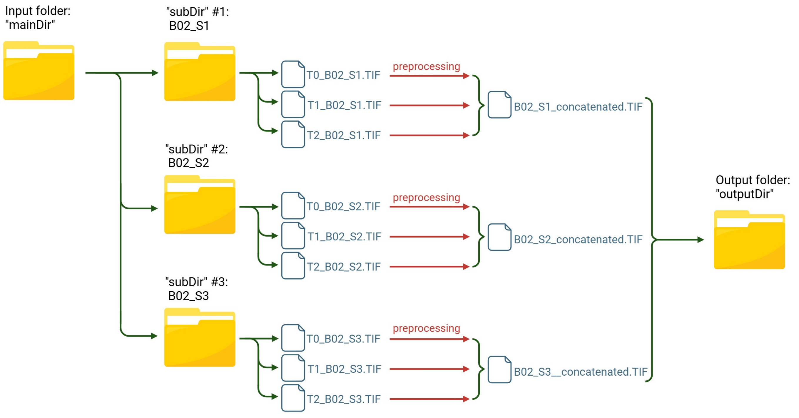
Figure 5. Workflow of the “survival_preprocess” macro for image preprocessing and concatenation. Images from each field of view stored in individual subfolders are preprocessed and merged into a single concatenated file, which is saved in the output directory.
Image preprocessing procedure:
1. Open the “survival_preprocess” macro file by dragging and dropping it onto the Fiji toolbar. This action launches the Script Editor with the macro code already loaded.
2. Click on the Run button in the Script Editor window to execute the macro.
3. Upon execution, a series of dialog windows will prompt the user to specify required parameters, such as:
a. The mainDir (the input folder, containing subfolders: each subfolder represents a set of images, such as all the time points for a specific FOV).
b. The outputDir (the output folder where the results will be saved: the concatenated stack).
c. The minimum area value, measured in pixels (px), is associated with the Gray Scale Attribute Opening step at line 56 of the code. The user can input a numeric value, with a default set to 500 (Figure 6).

Figure 6. Screenshot of the menu to set the area value for Gray Scale Attribute filtering. Setting the minimum area value, measured in pixels (px), associated with the Gray Scale Attribute Opening processing step.
4. The code will autonomously perform the following steps:
a. For each subfolder found in the main input folder, the macro code checks whether it is indeed a folder.
b. Inside the subfolder:
i. It opens each image.
ii. It applies Despeckle (a median filter that replaces each pixel with the median value in its 3×3 neighborhood) to remove salt and pepper noise from the image (https://imagej.net/ij/docs/menus/process.html).
iii. It applies Gray Scale Attribute Filtering with a morphological opening based on a minimum area of 500 pixels as the default value.
CRITICAL: The minimum value of the attribute, expressed in pixels, should be optimized for the images by the operator. It is a specific command of the MorphoLibJ plugin in Fiji that aims to remove components of the grayscale image based on a certain size criterion, rather than on intensity. We set up the Gray Scale Attribute Filtering steps using ”opening” as a morphological size operation and “area” (number of pixels) as an attribute [8].
iv. It renames the image using the time point followed by “tp” (Figure 7).
v. It closes the original image.
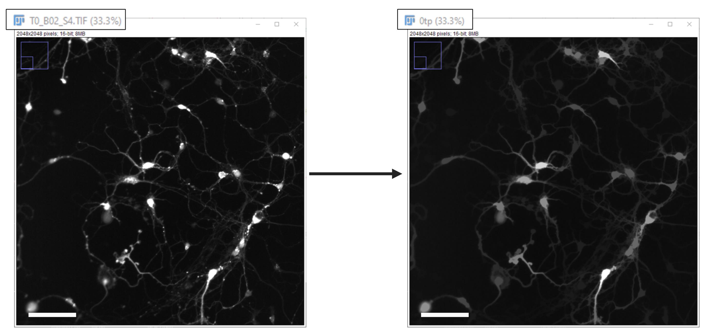
Figure 7. Despeckle and gray scale filtering. Enlarged portion of a single time point field of view, adjusted only for brightness and contrast, before and after image processing (Despeckle and Gray Scale Filtering). It is also shown how the image is renamed during processing. Scale bar, 100 µm.
c. After processing all the images in the subfolder, it concatenates them into a TIF file and saves it with the suffix “_concatenated”.
d. Once the macro execution is complete, a message will be displayed indicating that the process has finished.
K2. Cell survival analysis
Two macros, “no_loop” and “loop”, are available for survival analysis. Developed in Jython (.py), both are fully automated tools intended to quantify neuronal survival over time using morphological and intensity-based criteria. Specifically, the macros use the pre-trained StarDistDetectorFactory segmentation model [11] as a detector within Fiji’s TrackMate plugin [12] to segment single cells in the images. Please note that the TrackMate plugin does not require a separate download as it is already bundled with Fiji.
The “survival_analysis_no_loop” macro is designed for the initial setup phase, allowing the operator to test and fine-tune the detection parameters. It works on a single concatenated TIF file, which must be manually opened prior to execution. Once the analysis is complete, the macro will display the cells identified as “alive” at each time point with a colored overlay and will open a log window summarizing both the steps performed and the analysis results. This visual feedback enables the operator to assess the effectiveness of the chosen parameters.
Specifically, the log file generated for each concatenated image analyzed reports, for every time point of the concatenated image (defined as frame 0, 1, 2, etc.), the “spots total”, corresponding to the total number of cells detected by the plugin, and the “visible” spots, corresponding only to the cells that meet the selection criteria defined by the operator (Figure 8).
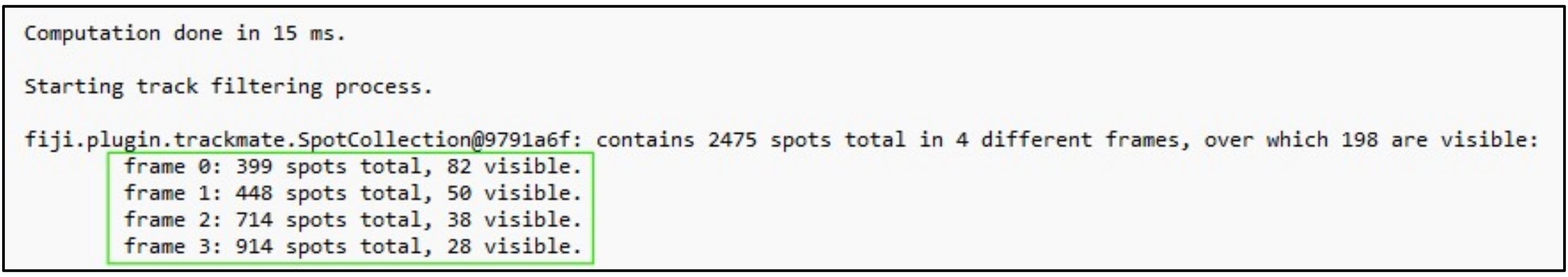
Figure 8. Screenshot showing the final section of the log file generated by the “survival_analysis_no_loop” macro. Framed in green are the numbers of total and visible spots (i.e., cells) per frame. Each frame corresponds to a single time point.
After validating the detection settings, the “survival_analysis_loop” macro can be used to automatically process all concatenated TIF files in the input folder. Typically, this folder corresponds to the output directory of the “survival_preprocess” macro, which contains preprocessed and concatenated images (each file representing one field of view across multiple time points).
K2.1. Cell survival analysis procedure, using the “survival_analysis_no_loop” macro
1. Open the concatenated TIF file to be used for analysis by dragging and dropping it onto the Fiji toolbar.
2. Open the “survival_analysis_no_loop” macro file by dragging and dropping it onto the Fiji toolbar. This action will launch the Script Editor with the macro code loaded.
3. Click on the Run button in the Script Editor window to execute the macro.
4. The script will autonomously perform the following steps:
a. Displays a window where the user enters four values using four separate text fields, one for each parameter (area, shape, mean intensity, and contrast) (Figure 9).
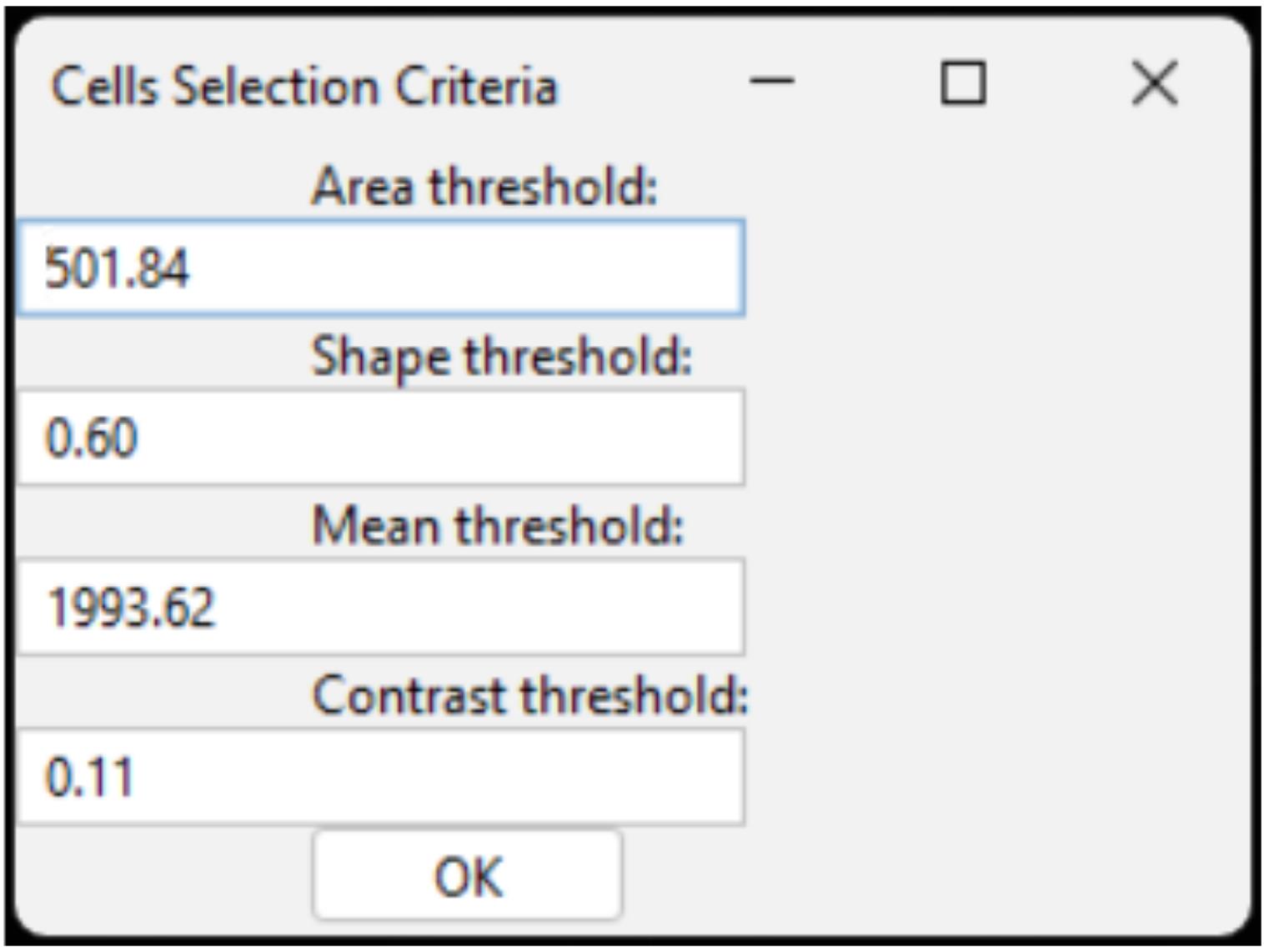
Figure 9. Cells selection criteria dialog window. Example of the interface used to set threshold parameters for cell selection, including area, shape, mean intensity, and contrast values.
CRITICAL: The values provided above (area > 501.84, shape > 0.60, mean intensity on channel 1 > 1993.62, contrast on channel 1 > 0.11) are intended as guidelines and should be adjusted as needed based on the specific characteristics of the images.
b. It creates a TrackMate model and utilizes the StarDistDetectorFactory, a deep-learning-based detector, to detect single cells.
c. It applies the four user-defined filters (area, shape, mean intensity, and contrast) on the detected cells.
d. Cell detection results are visualized in a hyperstack displayer. No interaction is required; display is part of the automated process (Figure 10).
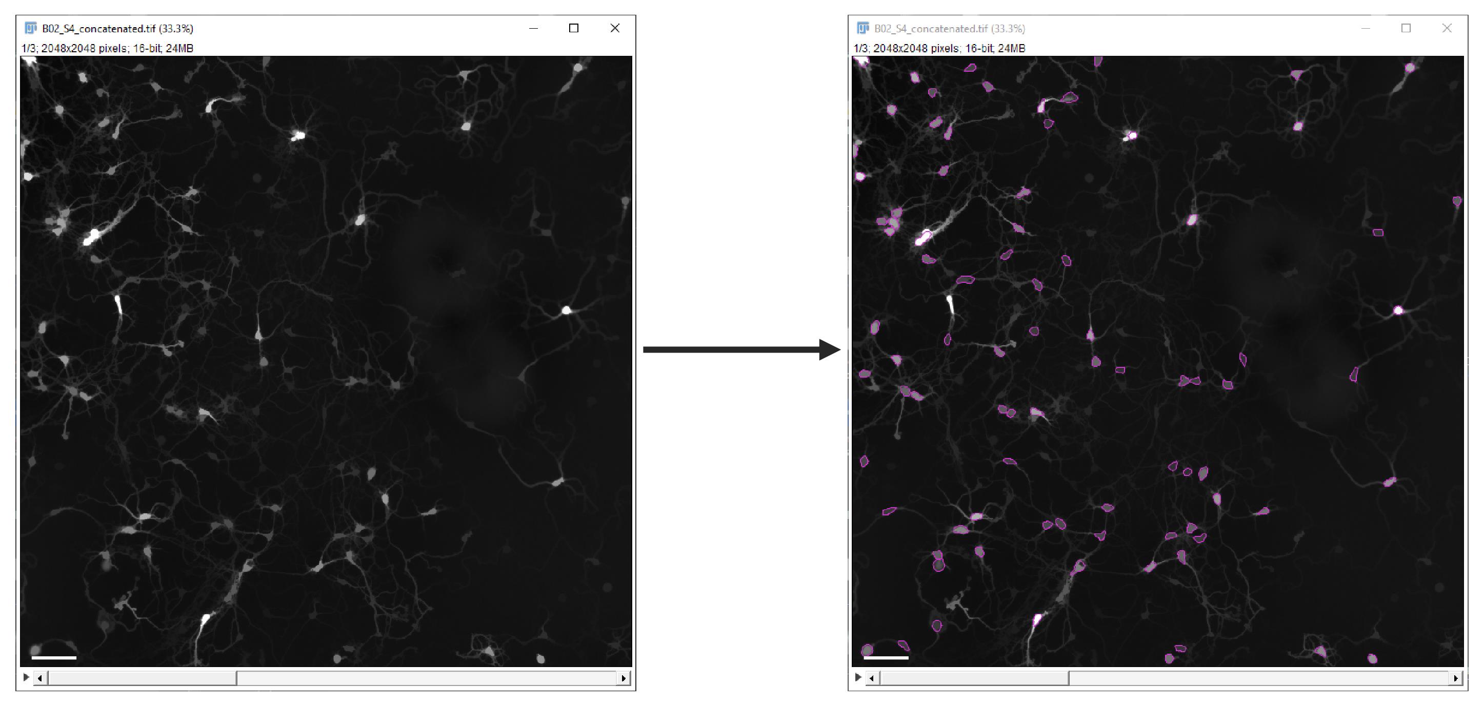
Figure 10. Cell detection results. Single time point field of view, before (left) and after (right) cell detection and selection. Scale bar, 100 µm.
e. For each concatenated file, the script logs the number of total and visible spots (cells) per frame.
K2.2. Cell survival analysis procedure, using the “survival_analysis_loop” macro
1. Open the “survival_analysis_loop” macro file by dragging and dropping it onto the Fiji toolbar. This action will launch the Script Editor with the macro code loaded.
2. Click on the Run button in the Script Editor window to execute the macro.
3. Upon execution, the macro displays a window where the user enters four values using four separate text fields, one for each selection parameter (area, shape, mean intensity, and contrast) (refer to step K2.1.4a for further details).
4. Select the input directory via a GUI prompt.
5. The script automatically creates an output subfolder (named “output”) within the selected input directory, which serves as the designated location for storing the results generated during the analysis.
CRITICAL: No other folder named “output” should be present in the input folder. If the folder already exists, this instruction will raise an error (i.e., OSError: [Errno 17] File exists: u’C:\\Data\\Experiment1\\output’).
6. The script will autonomously perform the following steps, looping through all TIF files in the selected input folder:
a. It opens each image.
b. It creates a TrackMate model and utilizes the StarDistDetectorFactory to detect single cells.
c. It applies the four user-defined filters (area, shape, mean intensity, and contrast) to the detected cells.
d. It closes all open images. Spot detection results are not displayed.
e. It logs the total and filtered (visible) number of spots (cells) at each time point, of each concatenated file.
7. Once looped over all the images present in the input directory, the macro parses the information reported in the log file to extract the image name and the number of visible spots at each time point. Subsequently, it calculates the ratio between the number of visible spots at each time point and the number of visible spots at T0.
8. The results are summarized in a table where each row contains the image name, the number of visible spots at each time point (T0, T1, T2, …), and the corresponding ratios (R0, R1, R2, …; with Rn = T0/Tn).
9. The table is saved as a .csv file named after the input directory, stored in the output folder. For example, if the input directory name is “images” and the output folder is “output”, the file “images.csv” will be created in the “output” folder.
10. The log file, which reports data about all the concatenated images present in the input directory, is also saved. This file is also named after the input directory name (e.g., images_log.txt) and stored in the “output” folder.
11. Once the macro execution is complete, a message will be displayed indicating that the process has finished.
L. Data analysis
At this point, all the images are processed and analyzed, and all the data of interest related to neuronal survival (the number of neurons in each field of view at every time point and the relative ratios) are summarized in a single .csv file.
L1. Data visualization
The .csv files generated by the image analysis pipeline require a few preparation steps to enable clear data visualization when opened in Microsoft Office 365 or similar open-access software (Figure 11).
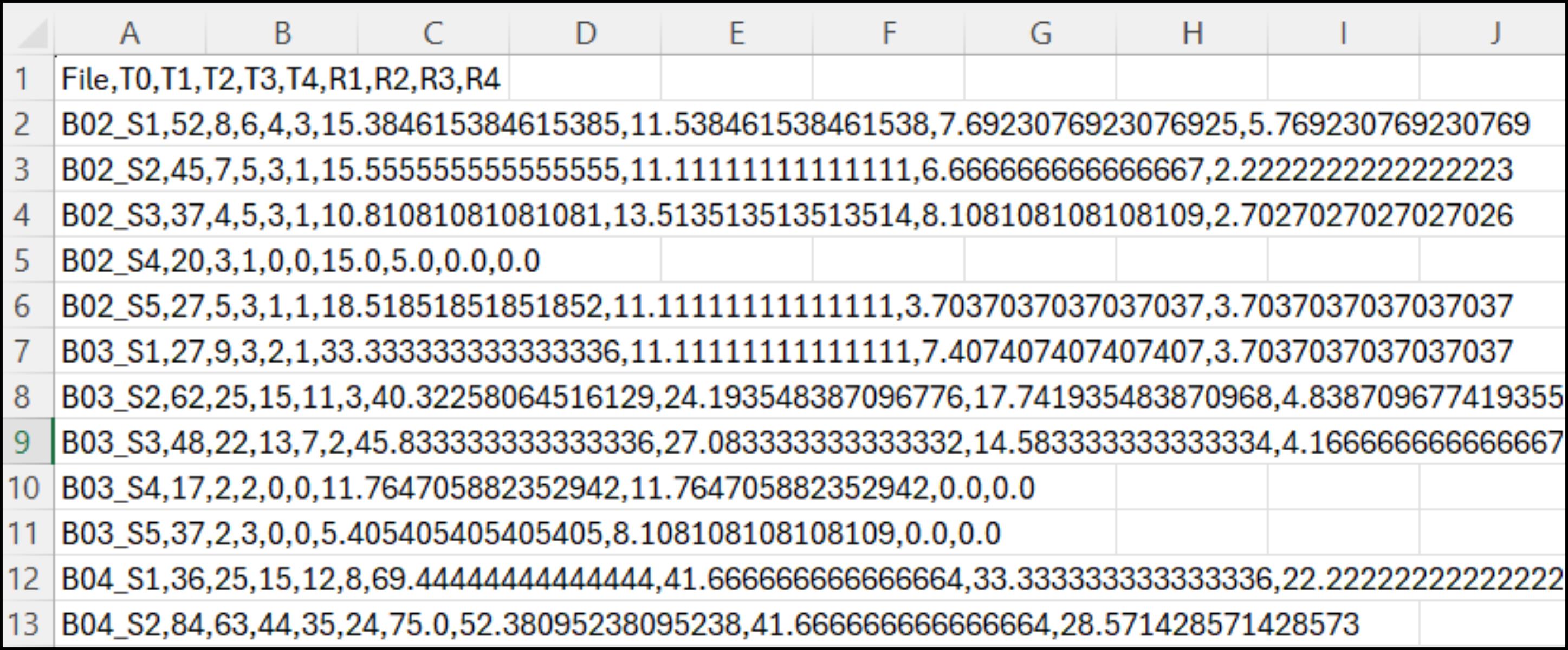
Figure 11. Example of the .csv file generated by the image analysis pipeline, opened in Microsoft Office 365 or equivalent tools. Each row corresponds to a specific field of view (e.g., B02_S1–B04_S1) and lists all the associated data in a comma-separated format.
To do so, proceed as follows:
1. Open the .csv file.
2. Select the column with all the data (Column A).
3. Click on the Text to Columns icon in the Data window. A window will pop up, requiring three steps to proceed forward.
a. Flag Delimited as Original data type, then click Next >.
b. Flag Comma as Delimiter, then click Next >.
c. In the Advanced Text Import Settings pop-up window, select the period as Decimal separator and a blank space as Thousands separator. Then press Ok and Finish to finally expand all the one-column-compressed data in all the corresponding columns, as reported in Figure 12.
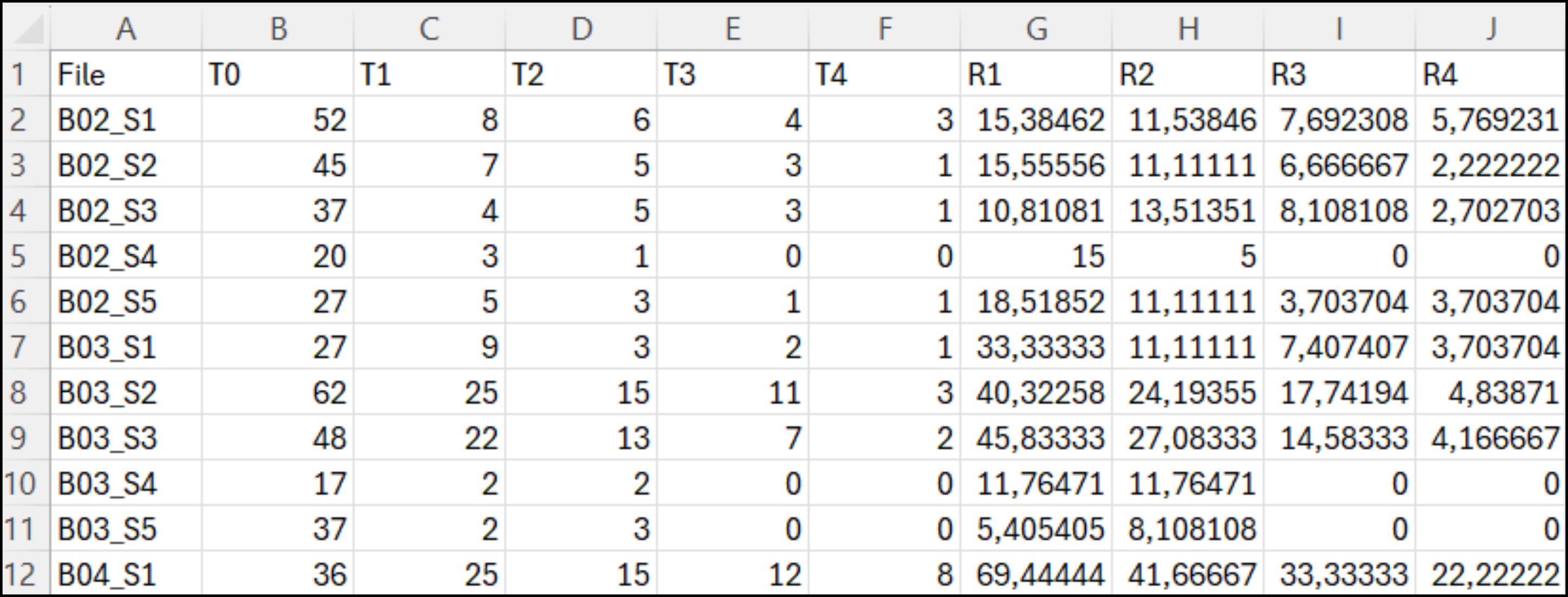
Figure 12. Representative .csv table, after manipulation for optimal visualization. Each row represents a specific sample (e.g., B02_S1–B04_S1), and each numerical data point is now presented in separate columns rather than as a single comma-separated line.
L2. Neuronal trophic effect detection
The first step of data analysis is crucial, and it involves determining the impact of the neuronal trophic effect on your data. Although the same number of neurons was seeded in each well, primary neuronal cultures are still affected by significant plating variability. This variability affects neuronal survival, as the greater the confluency of neurons, the greater their survival. For this reason, it is important to stratify the data according to the number of starting neurons in each FOV to enable a proper comparison between the different conditions and consider the contribution of the trophic effect.
To achieve this, a few steps are required, as follows:
1. From the .csv file previously generated, extract the number of neurons detected at T0 and group them for conditions in Excel or Prism. Check the range of starting neurons in each condition to verify if they have comparable ranges (Figure 13).
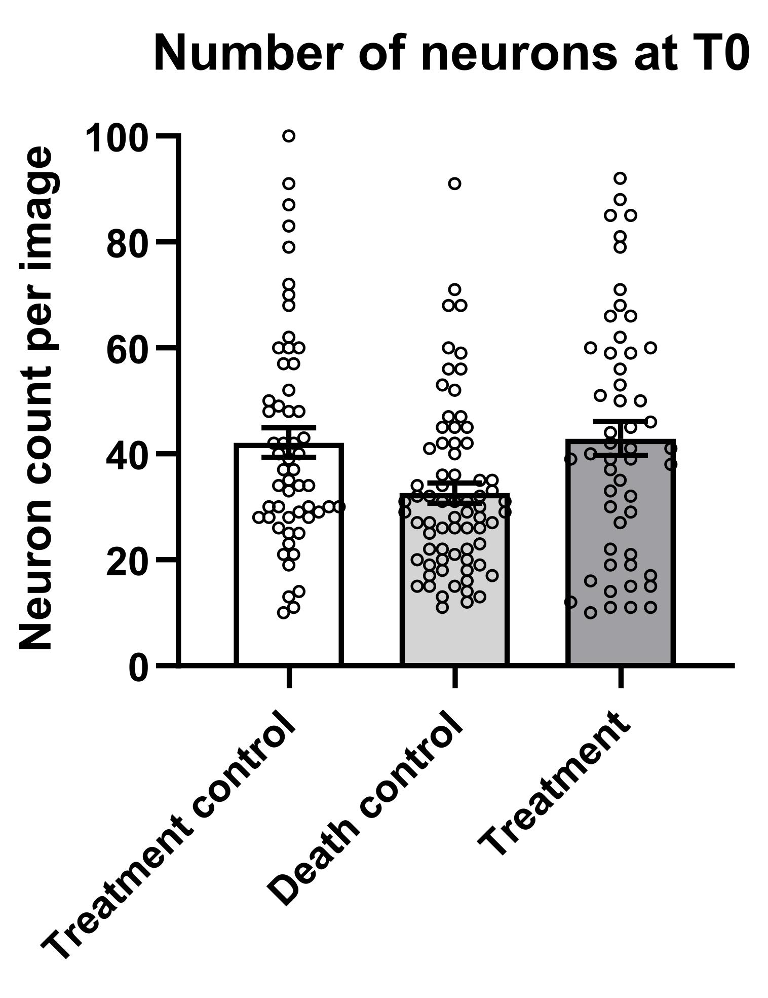
Figure 13. Starting number of neurons at T0 for each condition. Each point represents a specific field of view acquired at T0. Data represent mean ± SEM, n = 3 biological replicates, with over 50 fields of view acquired per condition.
2. From the .csv file, extract all the data referring to the treatment control and create a file with the initial number of neurons (T0) and all the related ratios (R0-Rn) for each FOV. Calculate the slope of the survival lines by applying linear regression on the data for each FOV, to obtain a simple parameter proportional to the rate at which the neurons are dying (Figure 14).
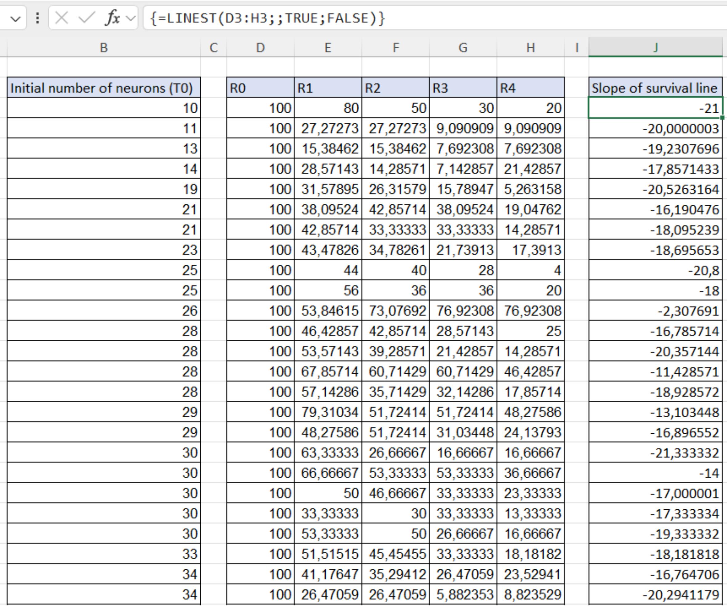
Figure 14. Calculation of the slopes of the survival lines. Calculations were obtained by applying linear regression to the data for each FOV acquired of the control condition.
3. Plot the initial number of neurons (T0) vs. the survival slopes to have a graph on which you can observe the trophic effect on neurons (Figure 15). In our case, we could divide the data into two main ranges: below and above 50 neurons. As you can see, below 50 neurons, there is a direct correlation between the starting number and the survival rate; however, above 50 neurons, a plateau is reached where the neurons appear to be unaffected by their number.
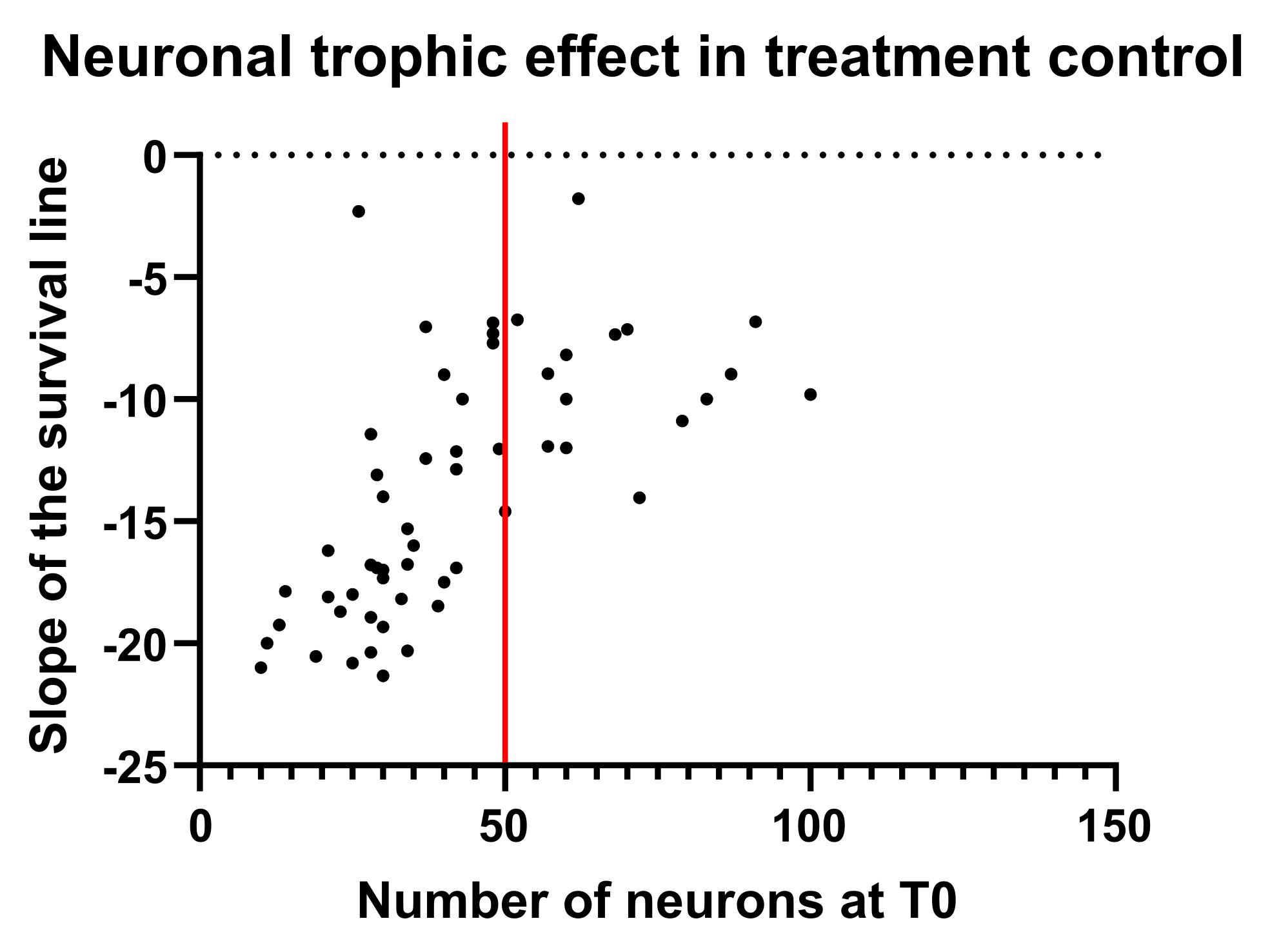
Figure 15. Neuronal trophic effect in treatment control. Each point represents the correlation between the starting number of neurons in a specific field of view and the slope of the survival line across time. The data can be divided into two main ranges: where a direct correlation between the starting number and the survival rate is present (before the red line), and where a plateau is reached, and neurons appear to be unaffected by their number (after the red line).
4. This clearly shows that failing to account for the neuronal trophic effect when comparing all conditions can lead to a misinterpretation of the data. For this reason, we strongly recommend stratifying the analysis according to the initial number of neurons. The upper range (plateau) could be useful for toxicity assays where neurons are known to be strong and healthy, while the lower range could be useful for experiments assessing the pro-survival properties of specific treatments. Depending on the number of FOV acquired, it is possible to divide the ranges into smaller ones to minimize the influence of the trophic effect as much as possible.
5. Once the ranges are defined, you can compare the survival percentages (Rn) of different conditions at each time point to identify significant differences between conditions. Treatment and death controls should always be included as indicative parameters in the analysis. Once data have been checked for normal distribution, it is possible to proceed with the statistical analysis. For example, if the distribution is normal, we recommend performing the analysis through a two-way ANOVA analysis followed by Tukey’s post hoc comparisons, since this will allow comparing all the conditions inside a specific timepoint but analyzing all the timepoints at the same time.
Validation of protocol
This innovative protocol was applied to perform a neuronal survival assay on primary cortical neurons to test the biological properties of astrocyte-derived extracellular vesicles (EVs) in a TDP-43Q331K murine model (Figure 7e of [1]). It was observed that the treatment with EVs derived from wild-type (WT) astrocytes induced a pro-survival effect on recipient neurons, compared to the treatment control (neurobasal), while this effect was lost when the neurons were treated with EVs derived from TDP-43Q331K astrocytes or MYC-overexpressing WT astrocytes.
General notes and troubleshooting
Troubleshooting
If the experimental cellular model used in the experiment changes, it is likely that some troubleshooting will be necessary to determine the optimal parameters throughout the entire protocol. Here, we present a table outlining the most common issues, their probable causes, and potential fixes.
| Main issues | Probable causes | Possible fixes |
|---|---|---|
| Low concentration of lentiviral particles | 1. Size of the lentiviral plasmid 2. Overconfluency of HEK293T cells | 1. If you are using a lentiviral plasmid that exceeds 10 kbp, it is possible that the transfection of HEK293T cells results in lower yields: try using a smaller plasmid. 2. Increase accuracy in cell counting when plating; overconfluency reduces transfection yields. |
| Overconfluency of plated cells | 1. Low accuracy in cell counting 2. Cells show a higher percentage of attachment and survival after plating | 1. Be sure the cells are well resuspended, without major agglomerates. 2. Try reducing the number of plated cells to achieve optimal confluency. |
| Cells look unhealthy after transduction | Lentiviral transduction affects cell survival, especially due to the necessity to remove the whole media the day after transduction | If the volume of viral particles used exceeded 10 μL/well, please try using a more concentrated virus to avoid additional toxicity due to excessive non-neuronal-specific media. Another option is lowering the MOI to increase survival. |
| Low amount of mCherry-positive cells | 1. Overconfluency of cells reduces the transduction yield 2. Some cell lines have higher resistance to transduction | 1. Try reducing the number of plated cells to achieve optimal confluency. 2. Try increasing the MOI to increase transduction yield, monitoring cell health. |
| The image analysis macros do not detect the cells correctly | The image analysis parameters are not properly set | Use a small pool of images, starting from the controls, to assess the best combination of parameters. First, be sure that the preprocessing is performing correctly, without creating issues with excessive or insufficient processing. After that, try identifying what could be the main issue; for example, if cells featuring a lower fluorescence are not detected, try modulating the Mean Intensity threshold, and if some neurites are detected as somas, try modulating the Shape threshold. |
| Data stratification is not feasible | The trophic effect is affecting all the cells in a similar way | If the cells are sufficiently confluent, all conditions may reach a plateau, meaning the trophic effect influences all cells similarly. In that case, no stratification would be needed, and all the data could be compared. |
Supplementary information
The following supporting information can be downloaded here:
1. Scripts
Acknowledgments
We would like to thank Luisa Donini, Francesca Conci, and Anna Barbieri for their help with primary cultures. Authors’ contribution: Conceptualization, P.V.F., M.R., M.B.; Investigation, P.V.F., M.R.; Writing—Original Draft, P.V.F., M.R., E.S.; Writing—Review & Editing, P.V.F., M.R., E.S., M.B.; Funding acquisition, M.B.; Supervision, M.B.
This project received funding from the European Union’s Horizon 2020 research and innovation program under the Marie Sklodowska-Curie grant agreement No 752470 (to MB); a grant from the Italian Ministry of the University (PRIN 20229HKCRT to MB), a pilot grant from Fondazione AriSLA (SENALS to MB; EVTestInALS to MB, and GATTALS to MB); and the initiative “Dipartimenti di Eccellenza 2023-2027 (Legge 232/2016)” funded by the MUR. The Department CIBIO Core Facilities (IRBIO) is supported by the European Regional Development Fund (ERDF) 2014–2020 and 2021–2027. We would like to thank the CIBIO Advanced Imaging Core Facility (AICF) and Michael Pancher and Pamela Gatto of the CIBIO HTS Core Facility for their assistance with the acquisitions using ImageXpress®. The protocol refers to results published in the Brain. 2025 Sep 26:awaf360. doi: 10.1093/brain/awaf360. Online ahead of print.
The following figures were created in BioRender: Graphical overview, Basso, M. (2025) https://BioRender.com/nd0zokw; Figure 2, Basso, M. (2025) https://BioRender.com/yapb54u; Figure 4, Roccuzzo, M. (2025) https://BioRender.com/ggwfl62; Figure 5, Roccuzzo, M. (2025) https://BioRender.com/4pym98k.
Competing interests
The authors declare no competing interests.
References
- Fioretti, P. V., Barbieri, A., Migazzi, A., Bressan, D., Grassano, M., Donini, L., Roccuzzo, M., Torrieri, M. C., Conci, F., Ferracci, E., et al. (2025). MYC-driven gliosis impairs neuron-glia communication in amyotrophic lateral sclerosis. Brain. e1093/brain/awaf360. https://doi.org/10.1093/brain/awaf360
- Young, L., Bilsland, J. and Harper, S. (1999). A rapid method for determination of cell survival in primary neuronal DRG cultures. J Neurosci Methods. 93(1): 81–89. https://doi.org/10.1016/s0165-0270(99)00134-x
- Aras, M. A., Hartnett, K. A. and Aizenman, E. (2008). Assessment of Cell Viability in Primary Neuronal Cultures. Curr Protoc Neurosci. 44(1): ens0718s44. https://doi.org/10.1002/0471142301.ns0718s44
- Rodríguez-Prieto, Ã., González-Manteiga, A., Domínguez-Canterla, Y., Navarro-González, C. and Fazzari, P. (2021). A Scalable Method to Study Neuronal Survival in Primary Neuronal Culture with Single-cell and Real-Time Resolution. J Visualized Exp. 173: e3791/62759. https://doi.org/10.3791/62759
- Migazzi, A., Scaramuzzino, C., Anderson, E. N., Tripathy, D., Hernández, I. H., Grant, R. A., Roccuzzo, M., Tosatto, L., Virlogeux, A., Zuccato, C., et al. (2021). Huntingtin-mediated axonal transport requires arginine methylation by PRMT6. Cell Rep. 35(2): 108980. https://doi.org/10.1016/j.celrep.2021.108980
- Vermeire, J., Naessens, E., Vanderstraeten, H., Landi, A., Iannucci, V., Van Nuffel, A., Taghon, T., Pizzato, M. and Verhasselt, B. (2012). Quantification of Reverse Transcriptase Activity by Real-Time PCR as a Fast and Accurate Method for Titration of HIV, Lenti- and Retroviral Vectors. PLoS One. 7(12): e50859. https://doi.org/10.1371/journal.pone.0050859
- Schindelin, J., Arganda-Carreras, I., Frise, E., Kaynig, V., Longair, M., Pietzsch, T., Preibisch, S., Rueden, C., Saalfeld, S., Schmid, B., et al. (2012). Fiji: an open-source platform for biological-image analysis. Nat Methods. 9(7): 676–682. https://doi.org/10.1038/nmeth.2019
- Legland, D., Arganda-Carreras, I. and Andrey, P. (2016). MorphoLibJ: integrated library and plugins for mathematical morphology with ImageJ. Bioinformatics. 32(22): 3532–3534. https://doi.org/10.1093/bioinformatics/btw413
- Weigert, M., Schmidt, U., Boothe, T., Müller, A., Dibrov, A., Jain, A., Wilhelm, B., Schmidt, D., Broaddus, C., Culley, S., et al. (2018). Content-aware image restoration: pushing the limits of fluorescence microscopy. Nat Methods. 15(12): 1090–1097. https://doi.org/10.1038/s41592-018-0216-7
- TensorFlow Developers. (2025). TensorFlow (v2.20.0). Zenodo. https://doi.org/10.5281/ZENODO.4724125
- Schmidt, U., Weigert, M., Broaddus, C. and Myers, G. (2018). Cell Detection with Star-Convex Polygons. In A. F. Frangi, J. A. Schnabel, C. Davatzikos, C. Alberola-López, and G. Fichtinger (Eds.), Medical Image Computing and Computer Assisted Intervention – MICCAI 2018 (Vol. 11071, pp. 265–273). Cham: Springer International Publishing. https://doi.org/10.1007/978-3-030-00934-2_30
- Ershov, D., Phan, M. S., Pylvänäinen, J. W., Rigaud, S. U., Le Blanc, L., Charles-Orszag, A., Conway, J. R. W., Laine, R. F., Roy, N. H., Bonazzi, D., et al. (2021). Bringing TrackMate into the era of machine-learning and deep-learning. Bioinformatics. e458852. https://doi.org/10.1101/2021.09.03.458852
Article Information
Publication history
Received: Oct 28, 2025
Accepted: Dec 18, 2025
Available online: Jan 8, 2026
Published: Feb 5, 2026
Copyright
© 2026 The Author(s); This is an open access article under the CC BY-NC license (https://creativecommons.org/licenses/by-nc/4.0/).
How to cite
Fioretti, P. V., Roccuzzo, M., Saccon, E., Pennuto, M. and Basso, M. (2026). High Content In Vitro Survival Assay of Cortical Neurons. Bio-protocol 16(3): e5582. DOI: 10.21769/BioProtoc.5582.
Category
Neuroscience > Basic technology > High-throughput screening
Cell Biology > Cell viability > Cell survival
Cell Biology > Cell imaging > Live-cell imaging
Do you have any questions about this protocol?
Post your question to gather feedback from the community. We will also invite the authors of this article to respond.