- Protocols

- Articles and Issues
- For Authors
- About
- Become a Reviewer

A Reproducible Method to Evaluate Sublethal Acoustic Stress in Aquatic Invertebrates Using Oxidative Biomarkers
Published: Vol 16, Iss 2, Jan 20, 2026 DOI: 10.21769/BioProtoc.5581 Views: 177
Reviewed by: Noelia ForesiAnonymous reviewer(s)
Original research article
The authors used this protocol in:

Jan 2024

Protocol Collections
Comprehensive collections of detailed, peer-reviewed protocols focusing on specific topics


Related protocols
Abstract
Underwater noise is a growing source of anthropogenic pollution in aquatic environments. However, few studies have evaluated the impact of underwater noise on aquatic invertebrates. More importantly, studies involving early developmental stages have been poorly addressed. Significant limitations are due to the lack of standardized protocols for working in the laboratory. Particularly, the design of uniform procedures in the laboratory is important when working with species that inhabit short-term changing habitats, such as estuaries, which makes it difficult to carry out repeated experiments in the natural habitat. Besides, controlling for environmental variables is also important when assessing the effect of a stressor on the physiological parameters of individuals. This experimental protocol addresses that gap by offering an adaptable laboratory-based method to evaluate sublethal physiological responses to sound exposure under highly controlled conditions. Here, we present a reproducible and accessible laboratory protocol to expose crabs to recorded boat noise and evaluate physiological responses using oxidative stress biomarkers. The method is designed for ovigerous females, as we evaluated the effects on embryos and early life stages (i.e., larvae), but it can be readily adapted to different life stages of aquatic invertebrates. A key strength of this protocol is its simplicity and flexibility: animals are exposed to noise using submerged transducers under well-controlled laboratory conditions, ensuring consistency and repeatability. Following exposure, tissues or whole-body samples can be processed for a suite of oxidative stress biomarkers—glutathione-S-transferase (GST), catalase (CAT), lipid peroxidation (LPO), and protein oxidation. These biomarkers are highly responsive, cost-effective indicators that provide a sensitive and early readout of sublethal stress. Together, the exposure and analysis steps described in this protocol offer a powerful and scalable approach for investigating the physiological impacts of underwater noise in crustaceans and other aquatic invertebrates.
Key features
• Enables measurement of oxidative stress markers across different life stages—from embryos to larvae and adult tissues—offering a complete view of physiological impact.
• Ensures consistent, reproducible conditions through standardized exposure and sampling, supporting reliable comparisons across experiments.
• Flexible protocol adaptable to Neohelice granulata and other estuarine decapods or marine benthic invertebrates, broadening its applicability.
Keywords: Anthropogenic noiseGraphical overview

Background
Underwater noise pollution from motorboats and other human activities is increasingly recognized as a significant stressor in coastal and estuarine ecosystems [1]. Benthic crustaceans are especially vulnerable to acoustic disturbance due to their lifestyle, having restricted locomotion behaviors to escape from the noise source, compared to fish or marine mammals. While many previous studies have explored the behavioral and physiological effects of anthropogenic noise on marine vertebrates (see reviews for marine mammals [2] and fish [3]), standardized protocols for assessing oxidative stress responses across multiple developmental stages in invertebrates remain very limited (see review [4]). The semiterrestrial crab Neohelice granulata is a widely distributed and ecologically relevant species due to its role as an ecosystem engineer, serving as a valuable model for investigating the effects of underwater noise on its physiology [5]. This species is frequently exposed to fluctuating environmental conditions since it inhabits the intertidal zone of estuaries, salt marshes, and mangroves of the southwestern Atlantic Ocean, which implies a difficulty in carrying out experiments in the natural environment. This protocol addresses this gap by providing a controlled laboratory method to reproduce boat noise exposure and to measure oxidative stress biomarkers in embryos and larvae. Moreover, it could be extrapolated to studies involving adult tissues. Its reproducibility and adaptability make it a valuable tool for advancing research in marine ecotoxicology and understanding the sublethal effects of underwater noise on aquatic crustaceans.
Noise produced by motorized vessels is one of the most prevalent forms of underwater acoustic pollution. These vessels predominantly emit low-frequency sounds (10–500 Hz), which travel faster and farther underwater than in air, sometimes covering hundreds to thousands of kilometers and potentially affecting organisms across multiple ecological levels [6,7]. In benthic invertebrates—especially during early developmental stages—exposure to anthropogenic noise can disrupt physiological homeostasis, delay or accelerate developmental timing, and dysregulate stress-response pathways. For example, chronic boat-noise playback shortened embryonic development in N. granulata and produced physiological and biochemical changes in offspring (e.g., altered heart rate and elevated lipid peroxidation [8]). Similarly, repeated exposure to boat noise reduced embryo survival by approximately 20% in a marine gastropod, with corresponding impairments in larval viability [9]. Broad reviews of anthropogenic noise effects on marine biota also report that invertebrates exhibit changes in oxidative stress biomarkers, energy metabolism, and immune function when exposed to low-frequency noise [10]. For species like N. granulata, which inhabits shallow estuarine areas with frequent boat traffic, understanding the effects of this type of stressor is essential. The ability to evaluate oxidative stress responses in embryos and larvae under controlled conditions provides a robust framework for identifying early markers of sublethal stress and for examining how environmental challenges may influence different life stages. Conducting these experiments under controlled laboratory conditions is particularly important for estuarine species like N. granulata, as natural environments are highly dynamic, with substantial variability in temperature, salinity, oxygen levels, and other stressors that can fluctuate markedly within and between a few days. Laboratory-based approaches help isolate the effects of sound exposure from these confounding factors, enabling more accurate and reproducible assessment of the organism’s responses.
Despite the current growing evidence of noise impacts on aquatic invertebrates, there still remains a notable shortage of standardized laboratory protocols designed to investigate how such mechanical disturbances influence early life stages under controlled laboratory conditions [8,11]. This protocol was developed to help fill that gap. It offers a reproducible and accessible laboratory approach for exposing ovigerous females of N. granulata (and thus, subsequently embryos and larvae) to recorded boat noise. The setup uses submerged transducers to deliver sound in a controlled aquatic laboratory environment, ensuring consistency in exposure conditions across experiments. The method is straightforward and adaptable, allowing researchers to adjust exposure time, acoustic parameters, and sample type depending on the question at hand or the species involved. A major strength of this protocol lies in its integration with biochemical tools for evaluating organismal responses. Oxidative stress biomarkers—glutathione-S-transferase (GST), catalase (CAT), lipid peroxidation (LPO), and protein oxidation—provide early and sensitive indicators of physiological stress [12]. These markers are well-established in ecotoxicology: for instance, in octopus (Octopus vulgaris), coordinated increases in CAT, GST, and LPO were observed in digestive gland and arm tissues in response to metal exposure, validating their use as reliable biomarkers [13]. Similarly, studies in fish have documented that GST and CAT activities rise significantly under environmental stress (e.g., heavy metals or pharmaceuticals), preceding visible damage and correlating with pollutant levels [14]. Recent studies on sound exposure in N. granulata show that LPO, protein oxidation, and GST and CAT activities are biomarkers of oxidative stress under these conditions [5,8,15]. However, it is important to mention that the inclusion of other enzymes is also relevant, given that not all enzymes necessarily increase under stress. Moreover, these assays are relatively cost-effective, technically straightforward, and suitable for moderate-throughput screening. By combining acoustic exposure with these robust biochemical endpoints, this protocol delivers a versatile and scalable framework for investigating how anthropogenic noise affects aquatic invertebrates across life stages. Beyond its immediate application in physiology and toxicology, the protocol can be readily expanded to include behavioral assessments, multi-stressor designs (e.g., noise combined with temperature, hypoxia, or pollutants), and conservation-oriented questions. Its flexibility makes it suitable not only for laboratory-based mechanistic studies but also as a foundational tool for understanding broader ecological consequences of sound pollution in coastal and estuarine ecosystems.
Materials and reagents
Biological materials
1. Ovigerous adult Neohelice granulata females with embryos in an initial stage of development
Reagents
1. Milli-Q or distilled water
2. Absolute ethanol 99.5% Pro-análisis (ACS, Cicarelli, catalog number: 752)
3. Tris(hidroximetil)-aminometano hydrochloride (Tris-HCl) (Sigma-Aldrich, catalog number: T3253)
4. Bradford reagent (Sigma-Aldrich, catalog number: B6916)
5. Bovine serum albumin (BSA) (Sigma-Aldrich, catalog number: A9418)
6. Potassium phosphate dibasic (K2HPO4) MW 174.18 (Sigma-Aldrich, catalog number: 1.05104)
7. Potassium phosphate monobasic (KH2PO4) MW 136.1 (Sigma-Aldrich, catalog number: 1.05108)
8. 1-chloro-2,4-dinitrobenzene (CDNB) MW 202.55 (Sigma-Aldrich, catalog number: 237329)
9. L-Glutathione reduced (GSH) MW 307.3 (Sigma-Aldrich, catalog number: G6013)
10. Butylated hydroxytoluene (BHT) MW 220.35 (Sigma-Aldrich, catalog number: W218405)
11. Potassium chloride (KCl) MW 74.55 (Sigma-Aldrich, catalog number: P3911)
12. Acetic acid, glacial (Supelco, catalog number: 1.00066)
13. Sodium chloride (NaCl) MW 55.44 (Sigma-Aldrich, catalog number: S9888)
14. 2-Thiobarbituricacid (TBA) MW 144.15 (Supelco, catalog number: 1.08180)
15. Sodium dodecyl sulfate (SDS) MW 288.38 (Roche, catalog number: 11667289001)
16. 1-Butanol (Sigma-Aldrich, catalog number: 360465)
17. 1,1,3,3-Tetramethoxypropane (TMP) MW 164.20 (Sigma-Aldrich, catalog number: 108383)
18. Hydrogen peroxide (H2O2) MW 34.01 (Supelco, catalog number: 1.07298)
19. Tris(hidroximetil)aminometano (Tris-base) MW 121.14 (Sigma-Aldrich, catalog number: 252859)
20. Ethylenediaminetetraacetic acid (EDTA) MW 372.24 (Sigma-Aldrich, catalog number: E9884)
21. Hydrochloric acid (HCl) (Supelco, catalog number: 1.15186)
22. 2,4-dinitrophenylhydrazine (DNPH) (Sigma-Aldrich, catalog number: S548685)
23. Ethyl acetate (Sigma-Aldrich, catalog number: 319902)
24. Guanidine hydrochloride (Sigma-Aldrich, catalog number: G3272)
25. Sodium hydroxide (NaOH) MW 40 (Sigma-Aldrich, catalog number: 221465)
26. Trichloroacetic acid (TCA) MW 163.39 (Sigma-Aldrich, catalog number: T4885)
Solutions
1. Extraction buffer (Tris-HCl 0.1 M pH 7.8) (see Recipes)
2. Potassium phosphate buffer (see Recipes)
3. CDNB solution (see Recipes)
4. GSH solution (see Recipes)
5. Catalase reaction buffer (see Recipes)
6. BHT stock solution (see Recipes)
7. Homogenization buffer (KCl + BHT) (see Recipes)
8. Acetic acid solution (see Recipes)
9. 2-tiobarbituric acid (TBA) solution (see Recipes)
10. Sodium dodecyl sulfate (SDS) (see Recipes)
11. HCl solution (see Recipes)
12. DNPH reaction solution (see Recipes)
13. Trichloroacetic acid solution (see Recipes)
14. Ethanol-ethyl acetate solution (see Recipes)
15. Guanidine hydrochloride solution (see Recipes)
Recipes
1. Extraction buffer (Tris-HCl 0.1 M pH 7.8)
| Reagent | Final concentration | Quantity or volume |
|---|---|---|
| Tris-HCl, MW 157.6 | 0.1 M | 1.576 g |
| Distilled water | 100 mL |
2. Potassium phosphate buffer (Glutathione-S-Transferase reaction buffer or extraction buffer for carbonylation)
| Reagent | Final concentration | Quantity or volume |
|---|---|---|
| KH2PO4 | 0.05 M | 0.6805 g |
| K2HPO4 | 0.05 M | 0.871 g |
| Distilled water | 100 mL |
Adjust the pH to 7 using NaOH or HCl.
3. CDNB solution
| Reagent | Final concentration | Quantity or volume |
|---|---|---|
| CDNB | 50 mM | 0.01013 g |
| Ethanol absolute | 100% (v/v) | 1 mL |
| Total | 1 mL |
Prepare a 1 mL solution of CDNB by dissolving the reagent in absolute ethanol.
4. GSH solution
| Reagent | Final concentration | Quantity or volume |
|---|---|---|
| L-Glutathione reduced | 25 mM | 0.0115 g |
| Potassium phosphate buffer (Recipe 2) | 0.1 M | 1.5 mL |
| Total | 1.5 mL |
5. Catalase reaction buffer
| Reagent | Final concentration | Quantity or volume |
|---|---|---|
| Tris-base, MW 121.14 | 7.5 mM | 0.225 g |
| EDTA | 5 mM | 0.465 g |
| Distilled water | 250 mL | |
| Total | 250 mL |
6. BHT stock solution
| Reagent | Final concentration | Quantity or volume |
|---|---|---|
| BHT, MW 220.35 | 1.4 M | 15.4 g |
| Ethanol absolute | 50 mL | |
| Total | 50 mL |
7. Homogenization buffer (KCl + BHT)
| Reagent | Final concentration | Quantity or volume |
|---|---|---|
| KCl, MW 74.55 | 0.15 M | 0.575 g |
| BHT stock solution (1.4 M) (Recipe 6) | 0.035 M | 1.25 mL |
| Distilled water | Complete to 50 mL | |
| Total | 50 mL |
8. Acetic acid solution
| Reagent | Final concentration | Quantity or volume |
|---|---|---|
| Acetic acid | 20% | 10 mL |
| Distilled water | 40 mL | |
| Total | 50 mL |
Adjust the pH to 3.5 using NaOH.
9. TBA solution
| Reagent | Final concentration | Quantity or volume |
|---|---|---|
| TBA | 0.8% | 0.4 g |
| Distilled water | 50 mL | |
| Total | 50 mL |
Prepare a fresh TBA solution for each assay. Homogenize the solution at high temperature to fully dissolve the TBA. Allow it to cool to room temperature before use.
10. SDS
| Reagent | Final concentration | Quantity or volume |
|---|---|---|
| SDS | 560 mM | 4.05 g |
| Distilled water | 25 mL | |
| Total | 25 mL |
Do not store at 4 °C, as the solution will freeze.
11. HCl solution (2 M)
| Reagent | Final concentration | Quantity or volume |
|---|---|---|
| HCl, MW 36.46 | 2 M | 5.4 mL |
| Distilled water | 27.12 mL |
Must be prepared in a fume hood. To dilute concentrated acids, slowly add the acid to water while continuously stirring with a glass rod. Never pour water onto a concentrated acid!
12. DNPH reaction solution
| Reagent | Final concentration | Quantity or volume |
|---|---|---|
| DNPH, MW 198.14 | 10 mM | 0.0278 g |
| HCl 2 M | 14 mL |
To dilute concentrated acids, slowly add the acid to water while continuously stirring with a glass rod. Never pour water onto a concentrated acid!
13. Trichloroacetic acid solution (28%)
| Reagent | Final concentration | Quantity or volume |
|---|---|---|
| TCA, MW 163.39 | 10.5 g | |
| Distilled water | 37.5 mL |
Dissolve the TCA in 30 mL of distilled water and, after complete dissolution, adjust the volume to 37.5 mL.
14. Ethanol-ethyl acetate solution (1:1)
| Reagent | Final concentration | Quantity or volume |
|---|---|---|
| Ethanol | 125 mL | |
| Ethyl acetate | 125 mL |
Must be prepared in a fume hood.
15. Guanidine hydrochloride solution (6 M)
| Reagent | Final concentration | Quantity or volume |
|---|---|---|
| Guanidine hydrochloride, MW 95.53 | 15.762 g | |
| Distilled water | 27.5 mL |
Dissolve guanidine hydrochloride in 15 mL of distilled water and, after complete dissolution, adjust the volume to 27.5 mL. Must be prepared in a fume hood.
Laboratory supplies
1. 96-well flat-bottom microplates (Corning, catalog number: 353072)
2. 1.5-mL tubes (Eppendorf, catalog number: HS4323)
3. 50-mL tubes (Corning, catalog number: CLS430290)
4. Aluminum foil or paper towel (to shield plates from light)
5. Micropipettes (1–10, 20–200, 100–1,000 μL) and sterile tips
6. UV-transparent 96-well microplates (Corning, catalog number: CLS3635)
Equipment
1. Table centrifuge (Eppendorf, model: centrifuge 5418)
2. Vortex (VornadoTM, Benchmark Scientific, catalog number: BV101-B)
3. Spectrophotometer UV-VIS (BioTek EPOCH)
4. Water bath or dry block incubator at 25 °C
5. Stereomicroscope (Lancet, model: 217B)
6. Digital caliper (Starrett)
7. Tweezers (Labbox export)
8. Plankton net (Eisco, model: SKU BIO144)
9. Analytical balance (RADWAG AS 220.R2 220 g × 0.1 mg RS232)
10. Plastic aquarium (2 L, 20 × 15 × 15 cm) with perforated (squares of 1 cm2) walls, constructed with plastic mesh, fishing line, and plastic tape (Figure 1)
11. Circular PVC tank (600 L, 1.2 m diameter and 1.5 m depth)
12. Photoperiod (14:10) (Kalop)
13. Underwater loudspeaker (Lubell Labs Inc., USA, model: UW30, rated frequency response between 100 Hz and 10 kHz)
14. Power amplifier (American Pro, model: APXII-300, 230 V, 50 Hz)
15. Audio player: speaker or laptop with audio output
16. Hydrophone (Reson, model: TC4013, with a sensitivity response of -211 ± 3 dB re 1V/mPa between a wide frequency range of 1 Hz and 150 kHz)
17. Analogical-digital converter unit (Avisoft Bioacoustics, Avisoft UltraSoundGate 116 h digital acquisition card)
18. Preamplifier (1-MHz bandwidth single-ended voltage and a high-pass filter set at 10 Hz, 20 dB gain) (Avisoft Bioacoustics)
19. Laptop
Software and datasets
1. Avisoft Recorder USGH software (Avisoft Bioacoustics)
Procedure
A. Sound stimuli recording in a natural environment
Recording an underwater sound with the aim of reproducing it while preserving both its intensity and frequency structure in a controlled environment requires the use of calibrated systems. An underwater sound acquisition system consists of several components, which may be more or less integrated into a compact recorder. The key elements are:
1. Hydrophone: Its selection is crucial, as the sensitivity should be flat (or as flat as possible) across the frequency range of interest to ensure faithful reproduction. For high-quality hydrophones, the sensitivity curve is usually provided by the manufacturer at the time of purchase. This information, combined with the characteristics of the preamplifier, allows the recorded signal to be converted into accurate sound pressure levels.
2. Preamplifier: This component amplifies the signal generated by the hydrophone, which is typically very weak (on the order of a few millivolts). Since the preamplifier itself has a frequency response, it is essential to verify that the amplification is uniform across the frequency band of interest.
3. Analog-to-digital converter (ADC): Characterized mainly by its sampling rate and bit resolution. According to the Nyquist–Shannon sampling theorem, the acquisition frequency must be at least twice the maximum frequency of the signal to be reproduced. For example, if we aim to record a signal extending up to 20 kHz, the sampling frequency must be at least 40 kHz.
4. Data storage system and software: For instance, a computer equipped with dedicated acquisition software for recording and managing the signals.
After recording the stimulus from the natural environment, the first step is to characterize it, considering its energy distribution along its frequency extension. To assess the temporal evolution in both frequency and amplitude (e.g., using a spectrogram), the average spectral content, typically represented as the power spectral density (PSD), and the sound pressure level in a stated frequency band and time interval (SPL or Lp), have to be analyzed. To obtain a calibrated sound pressure level (Lp, re 1 μPa) of a recorded signal at a given frequency, the following equation can be applied:
where Vadc is the input voltage to the ADC, G is the linear gain of the preamplifier (dB), and S is the hydrophone sensitivity (V/µPa).
These measurements can be carried out in a selection of the original recording or after the application of specific filters able to isolate the exact stimulus to be tested (e.g., vessel noise, crustacean, or fish signals), and avoid possible co-presence of different sources of soundscape components, i.e., different geophonic conditions. This choice depends on the aim of the study.
Note: In [8], motorboat signals were selected, and no further filters were applied.
B. Selection of the acoustic stimulus to playback and construction of the playlists
Note: To strengthen the tests, it is advisable to include many recordings of the selected stimulus obtained from different days and hours to ensure genuine replication, reflecting the natural variability of the source, rather than relying on pseudo-replicates, which consist of repeated presentations of the same recording. An example, obtained from our protocol [8], is provided below, where 45 motorboat passes recorded from the Mar Chiquita coastal lagoon, during a previous soundscape study [16], were selected as the stimulus.
1. Select the audio files containing the most frequent and/or intense noise events of the selected stimulus recorded from the natural habitat of the study species or a similar noise environment.
2. Construct the playlists by randomly choosing different files from diverse days and hours to avoid pseudoreplication and ensure the building of a representative sound treatment.
3. Construct playlists containing 1 min of the sound stimulus + 1 min of silence. Use at least four different files of 1-min sound stimulus per playlist.
Note: In [8], we used burst broadband noise (with energy below and above 700 Hz), since this type of sound was identified as the most frequent and intense in the lagoon [17]. To construct the playlists, we use the Avisoft SAS Lab software.
4. Construct at least ten different playlists. The playlists constructed must be tested in the experimental system by using the underwater sound playback system.
C. Underwater sound playback system
A digital sound playback system typically consists of several key components:
1. Digital audio source/playback device: A computer or recorder storing the calibrated audio files (playlist) to be emitted.
2. Digital-to-analog converter (DAC): Converts the digital signal into an analog voltage.
3. Power amplifier: Increases the analog voltage to the level required by the projector. Its frequency response should be flat across the band of interest to avoid spectral distortion.
4. Underwater projector (speaker/transducer): Converts the amplified voltage into acoustic pressure in water. As with the hydrophone, the projectors transmit voltage response (TVR, dB re 1 μPa/V at 1 m) and must be considered to ensure faithful reproduction of signals across the frequency bands of interest.
5. Cabling and connectors: High-quality, waterproof cables to connect the components without introducing additional distortion or signal loss.
D. Experimental setup
1. Prepare the laboratory with an experimental room with controlled photoperiod and air temperature to avoid their effects on embryonic development. If it is possible, use anechoic walls to ensure acoustic insulation in the room.
2. Use an even number of experimental tanks, because one-half will be used for the controls and the other for the treatments.
3. Locate experimental tanks with anechoic walls at the maximum distance possible among them to avoid sound transmission. Use big experimental tanks of at least 600 L to improve noise transduction. Anechoic walls can be obtained by using expanded polystyrene diffusion panels (Vicoustic, http://www.vicoustic.com) (for more details, see [18]).
4. Fill the experimental tanks with water (seawater or freshwater, depending on the studied species). In case of salt water, control and maintain the same salinity throughout the experiment to avoid its effects on embryo development.
5. Maintain moderate aeration using aquarium-grade air pumps and diffusers to keep oxygenation without creating turbulence. Place aquarium-grade air pumps outside the experimental room to reduce noise levels.
6. Locate plastic aquariums (2 L, 20 × 15 × 15 cm) with perforated (squares of 1 cm2) walls (Figure 1) in each experimental tank by securing them with a fishing line attached to the experimental tank walls to ensure they all maintain the same distance from the transducer and are located just below the water surface (see Graphical overview).
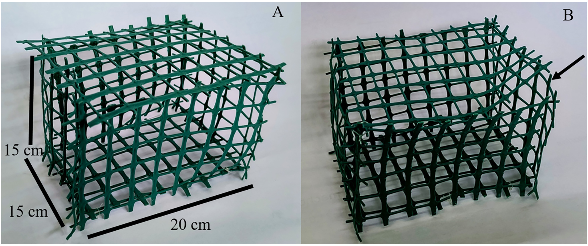
Figure 1. Plastic aquarium with perforated (squares of 1 cm2) walls. (A) Measurements of the aquarium. (B) Opening to put in and take out the crab (arrow).
7. Locate underwater transducers in the experimental tanks, in the center of the tank, suspended 30 cm from the bottom, in a horizontal position pointing at the surface. Secure the transducer with a thin rope (5 mm) to a wood plank (5 cm width and 2 m length) suspended above the experimental tank at a distance of 20 cm (Figure 2). From the experimental tanks, leave the same number of treatment and control tanks. The difference between treatment and control tanks is that in the first ones, the stimuli will be played by switching on the underwater sound playback system; in the control tanks, no sound emission will occur.
Note: In [8], a 14/10 h light/dark photoperiod was used to emulate natural environmental conditions. Water temperature was maintained at 17.5–18 °C, and filtered seawater at 33 PSU was used. The experimental tanks were made of PVC with 600 L capacity, 1 m diameter, and 1.15 m depth, filled with seawater at a depth of 0.8 m. Due to the laboratory facilities, four experimental tanks (two treatment and two control tanks) with six plastic aquariums inside each were used. Experimental tanks were placed at a distance of 4 m between them (one in each corner of the room) to avoid sound transmission. Plastic aquariums were constructed by using plastic mesh (perforations of 1 cm2 squares), which was cut with scissors into rectangles (15 × 20 cm) and squares (15 × 15 cm). Then, the aquarium was assembled by tying the walls with fishing line, leaving an opening to take out and put in the crab secured with plastic tape.
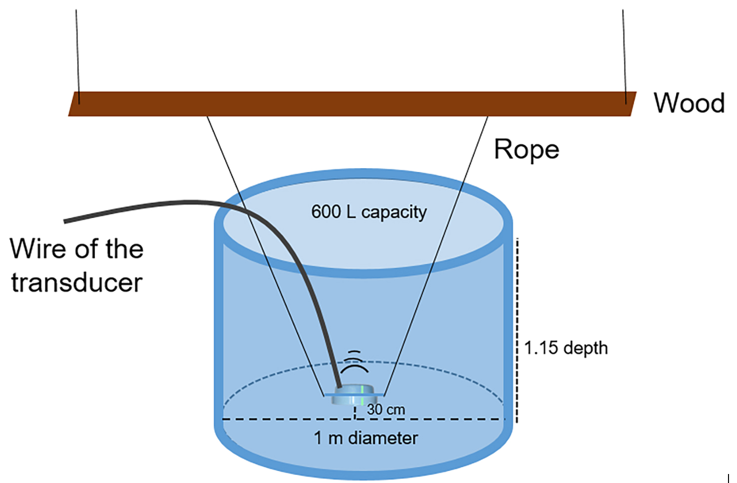
Figure 2. Experimental setup. Circular tank (600 L) with the transducer in its center, suspended 30 cm from the bottom, in a horizontal position pointing at the surface, secured with a thin rope (5 mm) to a wood plank (5 cm width and 2 m length) that is suspended above the tank at a distance of 20 cm.
E. Playlist reproduction and validation in the experimental system
The playlists constructed in section B must be transduced in the tank using the underwater sound playback system (section C) and recorded using the recording system (section A). The tank playlist recordings should be analyzed to assess their fidelity by comparison with the signal recorded in the natural environment. This comparison is typically performed by overlaying the power spectral densities (PSDs) of the natural and tank-recorded signals, and the results should be reported and carefully discussed in the manuscript. It is well known that a signal in a tank can never be identical to its natural counterpart: low frequencies are particularly difficult to reproduce due to the limited tank dimensions, and reflections from the walls and surface further alter the signal (see [19]). Nevertheless, this type of experimental setup offers considerable advantages, and imperfect reproduction is generally acceptable even if it needs to be discussed in the manuscript as an important limitation of the experiment. To reproduce the constructed playlists and validate the experimental system, the following procedure must be followed:
1. In the treatment tanks, place a hydrophone in the center at a depth of 30 cm from the bottom.
2. Couple the hydrophone with a preamplifier connected to a digital acquisition card and a laptop.
3. Connect the transducer to an amplifier plugged into an audio player.
4. Switch on all the equipment and ensure that all devices function properly.
5. Set the recording software (i.e., Avisoft Recorder USGH software, Avisoft Bioacoustics) to acquire the acoustic stimulus, using a sampling frequency of at least twice the maximum frequency of the signal to be reproduced, with 16-bit resolution.
6. Record the tank background noise for about 5 min with all devices switched on but no playlist being emitted.
7. Record the different playlists constructed.
8. Repeat the previous steps but place the hydrophone in the control tanks to check that there is only background sound and that no sound stimulus potentially coming from the treatment tanks is registered.
9. Calculate different sound parameters: the sound pressure level (Lprms) of the playlists emitted averaged over time, the power spectral density (PSD) of each emitted playlist, and the averaged PSD across all playlists. Measure the background noise in the tank to assess whether the animals were exposed to any sound during control conditions and to confirm that these noise levels were considerably lower than the playback stimuli. Measure the PSD of the tank background noise and that of the original playlists to compare the emitted sounds with those recorded in the natural habitat.
Note: In [8], data were analyzed using the PamGuide tool in MATLAB software [20]. The sound exposure level (SEL), measured over the exposure period, was calculated as the time-integrated squared sound pressure, normalized to one second, to quantify the total acoustic energy over time.
F. Experimental procedure
1. Capture ovigerous females with recently spawned eggs (i.e., embryos at stage one: 0–12 h post-extrusion).
Note: In [8], recently spawned females were captured from the Mar Chiquita coastal lagoon during the reproductive season (September–March) following characterization of embryo stages in [21].
2. Transport to the laboratory.
3. Measure the carapace width (maximum width) of females with a digital caliper to work with similar-sized individuals.
Note: In [8], recently spawned females ranged from 24 to 33.1 mm of carapace width.
4. Place each female individually in a plastic aquarium by using the opening and then close it by securing it with plastic tape.
5. Acclimate the crabs for 24 h, avoiding any handling or additional stress during this period.
6. Begin the experiment by starting playlist emission in the treatment tanks equipped with transducers by using the “loop mode” of the VLC media player software. Emit the playlist at a determined time each day, emulating the natural sound exposure of the studied species.
Note: In [8], a different playlist was reproduced each day for 12 h, from 7 am to 7 pm, as motorboat passes are frequent in the Mar Chiquita lagoon. Considering the total 10 playlists and the duration of the experiment, which extended beyond the embryonic development period of N. granulata (approximately 20 days under non-stressful conditions), playlists were subsequently reproduced again in the same order as previously used.
7. Feed the ovigerous females three times per week, removing food debris after feeding by using a net.
8. Partially change the water (half tank) three times a week.
9. Maintain the individuals in the experiment during full embryonic development until larval hatching. One day before hatching, place the females individually into unperforated aquaria to contain the larvae; see section G.
Note: In [8], females were fed with rabbit food pellets. To increase the data, and depending on the laboratory facilities (in our protocol, four tanks: two control and two treatments), the experiment is repeated twice in two consecutive months.
10. The experiment begins the same day for all females with embryos in stage 1 and ends on the particular day on which the larvae of each female hatch.
G. Sampling procedure
1. Control daily ovigerous females by visual inspection of the color of eggs.
2. Every two days, take a sample of eggs (i.e., embryos) from each female, using tweezers from the inside and outside of the egg mass, and observe them under a stereomicroscope to determine the embryos’ developmental stage.
3. Obtain samples of embryos in different advanced stages from each female using tweezers (both from control and treatment groups), weigh them on an analytical balance until a weight of 0.1 g is obtained, rinse them in distilled water, and store at -80 °C until processing for biochemical analysis.
Note: In [8], a sample of 30 embryos from each female was obtained to determine their developmental stage. The samples of embryos to be processed for the biochemical analysis were obtained in advanced stages 6 and 8 and were sampled following [21]. In N. granulata, fecundity (number of eggs per clutch) is high, thus allowing us to obtain the mentioned samples without affecting normal embryonic development and larval hatching. For other egg-laying species, it is suggested to verify the specific fecundity to determine the size of the samples and ensure normal embryo development and larval hatching.
4. When embryos reach the last stage of development, i.e., immediately before larval hatching, remove the females from the plastic aquariums and the PVC tank and place them in individual, not perforated plastic aquariums (1 L) to contain and individualize the offspring of each female.
Note: In [8], females with embryos in stage 9 were removed, since this is the last stage before larval hatching. The offspring refers to the first stage of larval development, i.e., zoea I in this species.
5. Obtain samples of zoeae I from each female by removing the female from the not-perforated plastic aquarium and filtering the water in a plankton net to retain them. Rinse the larvae in distilled water, weigh them in an analytical balance until a weight of 0.1 g is obtained, and store at -80°C until processing for biochemical analysis.
H. Tissue homogenization and preparation of enzyme extracts
1. Pool tissue samples to increase the biomass (in our protocol: N = 3 female samples from the same tank were pooled).
2. Homogenize 0.025 g of each sample (embryos of different stages and larvae) in 0.3 mL of extraction buffer (see Recipe 1) and centrifuge the homogenate at 10,000× g for 15 min at 4 °C following [22] and modifications of [23].
3. Use the supernatant as the enzyme source for activity determinations of GST and CAT. Collect supernatants and store them at -80 °C for further analysis of protein determination and enzymatic activity using a microplate spectrophotometer.
I. Oxidative stress biomarker analysis
1. Protein determination for enzyme activity normalization: The Bradford assay [24] is a rapid colorimetric method for quantifying total protein. Coomassie Brilliant Blue G-250 exists in cationic (red), neutral (green), and anionic (blue) forms. Under acidic conditions, the dye is red (abs max: 490 nm); binding to basic and aromatic residues converts it to the stable blue anionic form detected at 595 nm. The intensity of the blue complex is proportional to protein concentration.
Note: Detergents, flavonoids, and strong alkaline buffers can shift the dye’s pH and interfere with the assay.
a. Preliminary dilution check:
i. Select 2–3 random supernatant samples.
ii. In separate wells, add 10 μL of each sample.
iii. Add 10 μL of extraction buffer to a blank well.
iv. Add 10 μL of 1 mg/mL BSA to a reference well.
v. Add 100 μL of Bradford reagent to each well, cover, incubate for 5 min at room temperature, and read absorbance at 595 nm.
vi. If any sample absorbance exceeds the highest point of the forthcoming BSA standard curve, dilute that sample with extraction buffer and repeat.
b. Standard curve and sample measurement (triplicates):
i. Prepare eight BSA standards (0.005, 0.01, 0.025, 0.05, 0.075, 0.10, 0.30, and 1.0 mg/mL) by diluting the stock in extraction buffer (Table 1).
Table 1. Preparation of the BSA standard curve
| BSA concentration (μg/μL) | BSA (μL) | Extraction buffer (μL) |
|---|---|---|
| 0.005 | 2.5 | 497.5 |
| 0.01 | 5 | 495 |
| 0.025 | 12.5 | 487.5 |
| 0.05 | 10 | 190 |
| 0.075 | 7.5 | 92.5 |
| 0.1 | 10 | 90 |
| 0.3 | 30 | 70 |
| 1 | 50 | 0 |
ii. Dispense 10 μL of blank (extraction buffer) into three wells.
iii. Dispense 10 μL of each BSA standard into three wells.
iv. Dispense 10 μL of each sample, in triplicate, into the remaining wells.
v. Using a multichannel or single-channel pipette, add 100 μL of Bradford reagent to every occupied well (9.6 mL of extraction buffer per full plate).
vi. Gently tap the plate or pulse briefly on a plate shaker, cover with foil, incubate for 5 min (20–25 °C), and measure absorbance at 595 nm.
Pause point: Once the Bradford reagent has been added, readings should be taken within 60 min for consistent color development.
c. Data analysis:
i. For blanks, calculate the mean of the A595nm value; subtract this value from all standards and samples.
ii. Plot corrected A595nm values vs. BSA concentration (x-axis) and perform a first-order linear regression. The curve is acceptable when R2 ≥ 0.95.
iii. Use the regression equation (y = ax + b) to solve for x (protein concentration) of each sample.
iv. If a sample is diluted, multiply the calculated concentration by its dilution factor (final volume/initial sample volume).
Example: 100 μL sample + 100 μL extraction buffer → final 200 μL; dilution factor = 2.
Critical: Always apply the dilution factor to the calculated protein value, never to the raw absorbance.
Troubleshooting:
Low R2 (<0.95): Prepare fresh standards and repeat the curve.
Unexpectedly high background: Verify buffer pH (7.0–7.4) and absence of interfering detergents.
Sample color outside standard range: Adjust protein concentration by further dilution and re-assay.
2. GST activity assay: GSTs are phase II detoxification enzymes that catalyze the conjugation of reduced glutathione (GSH) to electrophilic compounds via a thiol group, forming more water-soluble products for excretion. This assay is based on the GST-catalyzed reaction between CDNB and GSH, which forms a dinitrophenyl-thioether detectable by its increase in absorbance at 340 nm (ε = 9.6 mM-1·cm-1 at pH 6.5). The reaction is linear over time and correlates with GST activity in the sample.
Note: All steps should be performed under low light conditions to protect CDNB from degradation.Ensure all reagents are freshly prepared and equilibrated to 25 °C before beginning.
a. Reaction setup:
i. Pre-incubate 3.8 mL of potassium phosphate buffer (Recipe 2) in a 50 mL tube at 25 °C for 15 min.
ii. Add 80 μL of CDNB solution (Recipe 3) to the prewarmed buffer and mix gently.
iii. Aliquot 235 μL of this CDNB–buffer mixture into the wells of a 96-well microplate.
iv. Use only columns 1–3 (24 wells) to allow timely reagent addition and data acquisition before the reaction begins to plateau.
v. Include blank wells containing the extraction buffer instead of the sample.
b. Plate assembly:
i. Add 15 μL of sample or blank (reaction buffer) to each corresponding well.
ii. Add 10 μL of GSH solution (25 mM) (Recipe 4) to each well using a multichannel pipette.
iii. Gently tap the plate or briefly pulse in a shaker to ensure mixing.
iv. Immediately begin absorbance readings at 340 nm, recording data every 20 s for 4 min.
v. Maintain the plate at 25 °C during measurement.
vi. See Table 2 for the final reagent concentrations in the wells.
Table 2. Final reagent concentrations in each well
| Reagent | Volume to be pipetted (μL) | Final concentration |
|---|---|---|
| Samples and blanks | 15 | |
| CDNB 1 mM (in reaction buffer, see Recipe 3) | 235 | 0.90 mM |
| GSH 25 mM | 10 | 0.96 mM |
| Final volume (μL) | 260 |
c. Data analysis:
i. From the absorbance data, select a 180-s linear interval where R2 > 0.98 and calculate the change in absorbance (A340nminitial - A340nmfinal) per minute.
ii. Calculate enzyme activity using the Lambert–Beer law:
Where:
EA: Enzymatic activity
ΔA340/time: Absorbance change per minute
ε: Molar extinction coefficient of the thioether product at 340 nm = 9.6 mM-1·cm-1
ι: Optical path length; if not auto-corrected by the spectrophotometer, use 0.735 cm for 260 μL in standard microplate wells.
V total: Total reaction volume (0.260 mL)
V sample: Sample volume (0.15 mL)
[Protein] = sample protein concentration (mg/mL)
iii. Express GST activity as μmol/min/mg protein by dividing the calculated activity by the protein concentration of each sample.
Notes:
1. If samples were diluted prior to the assay, apply the dilution factor to the final calculated activity.
2. Some plate readers automatically correct pathlength; if so, omit the adjustment.
Troubleshooting:
Low or unstable signal: check the freshness of CDNB and GSH; ensure the water bath and plate temperature are stable at 25 °C.
Nonlinear readings: reduce reaction volume or re-check sample protein concentration; activity may be too high.
Absorbance drift in blanks indicates contamination or degraded reagents; prepare fresh buffer and blanks.
3. CAT activity assay: CAT is an antioxidant enzyme primarily located in peroxisomes and mitochondria, where it catalyzes the breakdown of hydrogen peroxide (H2O2) into water and oxygen, preventing oxidative damage. This assay estimates catalase activity by monitoring the decrease in absorbance at 240 nm, which corresponds to the consumption of H2O2. The reaction follows first-order kinetics, with the rate directly proportional to the H2O2 concentration. To maintain reaction linearity, the assay is performed with relatively low substrate concentrations (10–50 mM). The extinction coefficient of H2O2 at 240 nm is ϵ = 36 M-1·cm-1.
Note: H2O2 stability is critical; its quality and storage conditions may significantly affect assay performance.
Critical: H2O2 should be freshly diluted on the day of the experiment. Use light protection and avoid repeated freeze-thaw cycles. Pre-test the batch of H2O2 to determine the decay rate if needed.
a. Reaction mix preparation:
i. Prepare the catalase reaction buffer (see Recipe 5) in advance and store at 4 °C.
ii. On the day of the assay, dilute H2O2 in the buffer to reach a final concentration of 10 mM. For two plates, prepare ~50 mL of reaction mix (e.g., 51 μL of H2O2 in 49.95 mL of buffer).
iii. Equilibrate the mix to 25 °C before use.
Note: H2O2 concentration and quality can affect results. Record the exact concentration used. Different protocols may suggest different working ranges (10–100 mM), but lower concentrations are recommended for better linearity.
b. Plate setup and measurement:
i. Add 5 μL of sample or blank (buffer) to each well.
ii. Using a multichannel pipette, add 250 μL of prewarmed reaction mix to each well.
Note: Due to the fast kinetics, limit measurements to 2–3 columns at a time.
iii. Immediately start reading absorbance at 240 nm every 10 s for 2 min.
iv. Monitor blanks for unexpected absorbance changes. Repeat samples if necessary.
Notes:
1. Bubbles in wells after reagent addition may indicate very high catalase activity. Reduce sample volume or increase H2O2 concentration.
2. Lack of bubbles may suggest low CAT activity. Consider increasing sample volume or confirming H2O2 concentration.
3. Final well volume should be 255 μL. Adjust calculations accordingly if volumes differ.
c. Data analysis: Identify a 60-s linear interval with R2 > 0.95 and calculate the change in absorbance per minute (ΔA240/min). Use the Beer–Lambert law to calculate catalase activity:
Where:
ε: 36 M-1·cm-1 (extinction coefficient of H2O2)
ι: Optical pathlength (use 0.75 cm for 255 μL in standard wells)
V reaction: 0.255 mL
V sample: 0.005 mL
[Protein]: Sample protein concentration (mg/mL)
Express CAT activity as μmol H2O2 degraded per minute per mg protein. If samples were diluted, apply the dilution factor to the final result.
Troubleshooting:
Unstable readings or low activity: Check the freshness and concentration of H2O2; test buffer pH and ensure samples are kept cold prior to use.
Very rapid absorbance drop: Dilute the sample or reduce the pipetted volume.
No change in absorbance: Increase sample volume or H2O2 concentration.
High signal in blanks: Indicates reagent contamination or H2O2 degradation; prepare fresh solutions.
4. Lipid peroxidation (LPO), thiobarbituric acid reactive substances (TBARS) assay: The TBARS assay quantifies oxidative stress by measuring lipid peroxidation damage, which occurs through the generation of free radicals. Lipid peroxidation products derived from polyunsaturated fatty acids are stable and decompose into a complex mixture of compounds, including malondialdehyde (MDA). MDA reacts with thiobarbituric acid (TBA) under high temperature and acidic conditions to form a chromogen detectable by spectrophotometry or fluorometry. Originally standardized for evaluating oxidative damage in liver and gonad samples from fish, this method is now widely used in ecotoxicology.
a. Prepare BHT stock solution, homogenization buffer (KCl + BHT), acetic acid solution, TBA solution, and SDS (see Recipes 6, 7, 8, 9, and 10, respectively).
b. Prepare TMP standard curve:
i. Mix 5 μL of TMP with 15 mL of distilled water to create a 2 mM stock solution (Table 3). Do not store at 4 °C, as the solution will freeze.
Table 3. TMP stock solution
| Reagent | Final concentration | Quantity or volume |
|---|---|---|
| TMP | 2 mM | 5 μL |
| Distilled water | 15 mL | |
| Total | 20 mL | 15.005 mL |
ii. Prepare 8 serial dilutions ranging from 2 μM to 0.015 μM using 1:1 dilutions with distilled water (Table 4).
Note: Use vortexing at each step.
Table 4. Serial dilutions of TMP
| Standard | Final concentration | Preparation |
|---|---|---|
| Standard 1 | 2 μM | 10 μL of concentrated solution + 9.99 mL of distilled water |
| Standard 2 | 1 μM | 1 mL of standard 1 + 1 mL of distilled water |
| Standard 3 | 0.5 μM | 1 mL of standard 2 + 1 mL of distilled water |
| Standard 4 | 0.25 μM | 1 mL of standard 3 + 1 mL of distilled water |
| Standard 5 | 0.125 μM | 1 mL of standard 4 + 1 mL of distilled water |
| Standard 6 | 0.06 μM | 1 mL of standard 5 + 1 mL of distilled water |
| Standard 7 | 0.03 μM | 1 mL of standard 6 + 1 mL of distilled water |
| Standard 8 | 0.015 μM | 1 mL of standard 7 + 1 mL of distilled water |
| Blanck | 0 μM | 1 mL of distilled water |
Note: Store at room temperature; do not refrigerate.
c. Sample preparation: Homogenize 50 mg of tissue in 450 μL of homogenization buffer (KCl + BHT; 1:9 w/v).
d. Plate setup:
i. In glass tubes (duplicates), add 20 μL of homogenized sample.
ii. Add 20 μL of each TMP standard to separate tubes (duplicates).
iii. Add 20 μL of BHT stock only to sample tubes.
iv. Add 150 μL of 20% acetic acid solution to all tubes.
v. Add 150 μL of 0.8% TBA solution to all tubes.
vi. Add 50 μL of distilled water to sample tubes and 70 μL to standard tubes.
vii. Add 20 μL of SDS to all tubes.
viii. Vortex all tubes thoroughly.
ix. Incubate in a water bath at 95 °C for 30 min (cover with foil).
x. Let it cool for 10 min.
e. Extraction (in a fume hood):
i. Use cotton-plugged tips for pipetting.
ii. Add 100 μL of distilled water.
iii. Add 500 μL of 1-Butanol.
iv. Vortex and centrifuge at 3,000× g for 10 min at 15 °C.
v. Transfer 150 μL of the upper (organic) phase into a white 96-well microplate in duplicate.
vi. Measure fluorescence at 553 nm (excitation at 515 nm).
f. Data analysis:
i. Plot a linear regression of standard absorbance values (R2 > 0.95).
ii. Subtract blank absorbance from sample values.
iii. Calculate sample MDA concentration using the standard curve.
iv. Adjust the final concentration for dilution factors and normalize to protein content:
This protocol provides a sensitive and reliable method to quantify lipid peroxidation as a marker of oxidative stress in aquatic organisms. Its adaptability and robustness make it suitable for multiple tissue types and developmental stages.
5. Protein carbonylation quantification: Protein carbonylation is a widely recognized marker of oxidative damage in proteins. Free radicals generated during oxidative stress can attack enzymes and structural proteins, causing the formation of carbonyl groups (aldehydes and ketones) on protein side chains. These modifications may be primary, arising directly from metal-catalyzed oxidation or radiation, or secondary, resulting from reactions with oxidation products of other molecules.
The assay relies on the reaction of 2,4-dinitrophenylhydrazine (DNPH, also known as Brady’s reagent) with protein carbonyl groups, forming hydrazone derivatives that display a yellow to orange color. These derivatives absorb light in the 355–390 nm range, with a molar extinction coefficient (ϵ) of 2.2 × 10⁴ M-1·cm-1, allowing quantification by spectrophotometry.
a. Reagents and sample preparation:
i. Normalize protein concentration of samples to 2 mg/mL using catalase reaction buffer (Recipe 5).
ii. Prepare DNPH reaction solution (see Recipe 12) and corresponding blanks with 2 M HCl (see Recipe 11).
iii. Prepare 28% TCA solution, ethanol-ethyl acetate solution, and guanidine hydrochloride solution (see Recipes 13, 14, and 15, respectively).
b. Assay procedure:
i. Aliquot 200 μL of sample supernatant into two 2 mL tubes (100 μL for the test, 100 μL for the blank).
ii. Add 250 μL of 2 M HCl to blanks and 250 μL of DNPH reaction solution to test tubes.
iii. Incubate at 30–37 °C for 90 min in an incubator.
iv. Cool tubes on ice.
v. Add 350 μL of 28% TCA solution and vortex thoroughly.
vi. Centrifuge at 9,000× g for 10 min at 4 °C. Carefully discard supernatant.
vii. Resuspend the pellet in 500 μL of cold ethanol-ethyl acetate solution.
viii. Vortex and centrifuge again at 9,000× g for 10 min at 4 °C. Discard the supernatant carefully.
ix. Repeat washing steps I5vii–viii two or three times until supernatant is clear.
x. Resuspend pellet in 420 μL of guanidine hydrochloride solution.
xi. Incubate with shaking at 37 °C for 10 min.
xii. Centrifuge at 9,000× g for 3 min at 4 °C to remove insoluble material.
xiii. Transfer 200 μL of supernatant into microplate wells (duplicates or triplicates).
xiv. Measure absorbance at 355, 358, 370, and 390 nm.
Note: Depending on sample quality, select the wavelength corresponding to the absorption peak. A spectral scan (355–390 nm, in 5 nm increments) is recommended if available.
c. Data analysis:
i. Select the wavelength with the highest absorbance peak.
ii. Subtract blank absorbance from sample absorbance at the selected wavelength.
iii. Calculate protein carbonyl content using:
Where:
A355-390: Corrected absorbance
ε: 2.2 × 10⁴ M-1·cm-1, molar extinction coefficient
[Protein]: Protein concentration (mg/mL)
Results are expressed as nmol of DNPH incorporated per mg of protein.
Troubleshooting:
Inconsistent absorbance readings: Ensure reagents are fresh and that incubation conditions are consistent.
Pellet loss during washes: Carefully remove supernatant without disturbing the pellet.
Low absorbance signal: Verify protein concentration and reaction conditions.
Absorbance outside expected range: Confirm correct wavelength and check for instrument calibration.
Data analysis
The data obtained in the experiment may be analyzed separately for each trial, since the reproductive and physiological conditions of females (such as the number and size of embryos) can vary throughout the reproductive cycle [20].
Differences in GST and CAT enzymatic activities, as well as in lipid and protein oxidation levels, can be tested for each sample (embryos at stages 6 and 8 and zoea I) between the control and noise exposure treatments at both experimental dates, using t-tests after verifying the assumptions of normality and homoscedasticity.
Validation of protocol
This protocol has been successfully applied to evaluate oxidative stress biomarkers in embryos and larvae of N. granulata exposed to boat noise under controlled laboratory conditions [8]. The experimental design included four experimental tanks (two treatment and two control tanks) with six females inside each (in turn, each female was located in an experimental aquarium), and the experiment was repeated twice, in two consecutive months. Tissue samples from females of the same experimental tank were pooled (N = 3) to conduct the biochemical analysis. Thus, four replicates per the control and per the treatment in each experiment (one per month) were used.
The reliability and robustness of the protocol were confirmed through consistent and statistically significant differences in biomarker levels (e.g., GST, CAT, and TBARS) between control and noise-exposed groups. Data were analyzed using appropriate statistical tests (t-tests), and normality and homoscedasticity were verified before hypothesis testing.
This protocol (or parts of it) has been used and validated in the following research article(s):
Sal Moyano et al. [8]. Noise accelerates embryonic development in a key crab species: Morphological and physiological carryover effects on early life stages. Marine Pollution Bulletin.
General notes and troubleshooting
General notes
1. The protocol was optimized for N. granulata embryos and larvae, but it can be adapted to other estuarine or marine crustaceans.
2. The sound exposure setup should be carefully calibrated based on the selected stimulus, as variations in tank size, speaker position, or acoustic impedance can affect the intensity and distribution of the stimulus.
3. When working with embryos, the integrity of the egg capsule and stage of development must be confirmed under a stereomicroscope prior to biochemical analysis to ensure homogeneity among replicates.
4. All biochemical assays should be performed using freshly prepared reagents, and samples should be kept on ice during processing to minimize degradation.
5. Variability in oxidative stress biomarkers may arise from differences in maternal investment or embryo size; therefore, pooling individuals from multiple females (of the same trial) is recommended (see also section G).
Acknowledgments
We thank Agencia Nacional de Promoción Científica y Tecnológica (PICT, 2019-668) and Universidad Nacional de Mar del Plata (EXA 1213/24, PI2 RR, 1914/24). We are grateful to the CAIMAR Joint Laboratory Italy-Argentina (Laboratori Congiunti Bilaterali Internazionali) of the Italian National Research Council and the project BOSS: Study of bioacoustics and applications for the sustainable exploitation of marine resources (Projects of major importance in the Scientific and Technological Collaboration Executive Programs, funded by the Italian Ministry of Foreign Affairs and International Cooperation and the Argentinean Ministry of Science, Technology and Innovative Productivity). The work of Maria Ceraulo was performed within the project “National Biodiversity Future Center-NBFC” funded under the National Recovery and Resilience Plan (NRRP), Mission 4, Component 2 Investment 1.4-Call for tender No. 3138 of December 16, 2021, rectified by Decree no. 3175 of December 18, 2021, of Italian Ministry of University and Research funded by the European Union–NextGenerationEU. This protocol was used in [8].
Competing interests
The authors declare no conflicts of interest.
Ethical considerations
This study complies with the regulations of the National University of Mar del Plata (Argentina). According to the Committee for the Care and Use of Laboratory Animals (CICUAL), no specific legal requirements apply to research involving crabs in this institution.
References
- Duarte, C. M., Chapuis, L., Collin, S. P., Costa, D. P., Devassy, R. P., Eguiluz, V. M., Erbe, C., Gordon, T. A. C., Halpern, B. S., Harding, H. R., et al. (2021). The soundscape of the Anthropocene ocean. Science. 371(6529): eaba4658. https://doi.org/10.1126/science.aba4658
- Erbe, C., Reichmuth, C., Cunningham, K., Lucke, K. and Dooling, R. (2016). Communication masking in marine mammals: A review and research strategy. Mar Pollut Bull. 103: 15–38. https://doi.org/10.1016/j.marpolbul.2015.12.007
- Popper, A. N. and Hawkins, A. D. (2019). An overview of fish bioacoustics and the impacts of anthropogenic sounds on fishes. J Fish Biol. 94(5): 692–713. https://doi.org/10.1111/jfb.13948
- Solé, M., Kaifu, K., Mooney, T. A., Nedelec, S. L., Olivier, F., Radford, A. N., Vazzana, M., Wale, M. A., Semmens, J. M., Simpson, S. D., et al. (2023). Marine invertebrates and noise. Front Mar Sci. 10: e1129057. https://doi.org/10.3389/fmars.2023.1129057
- Snitman, S. M., Mitton, F. M., Marina, P., Maria, C., Giuseppa, B., Gavio, M. A. and Sal Moyano, M. P. (2022). Effect of biological and anthropogenic habitat sounds on oxidative stress biomarkers and behavior in a key crab species. Comp Biochem Physiol C Toxicol Pharmacol. 257: 109344. https://doi.org/10.1016/j.cbpc.2022.109344
- Peng, C., Zhao, X. and Liu, G. (2015). Noise in the Sea and Its Impacts on Marine Organisms. Int J Environ Res Public Health. 12(10): 12304–12323. https://doi.org/10.3390/ijerph121012304
- Erbe, C., Duncan, A. and Vigness-Raposa, K. J. (2022). Introduction to Sound Propagation Under Water. In: Erbe, C., Thomas, J.A. (eds) Exploring Animal Behavior Through Sound: Volume 1. Springer, Cham. 185–216. https://doi.org/10.1007/978-3-030-97540-1_6
- Sal Moyano, M. P., Mitton, F. M., Luppi, T. A., Snitman, S. M., Nuñez, J. D., Lorusso, M. I., Ceraulo, M., Gavio, M. A. and Buscaino, G. (2024). Noise accelerates embryonic development in a key crab species: Morphological and physiological carryover effects on early life stages. Mar Pollut Bull. 205: 116564. https://doi.org/10.1016/j.marpolbul.2024.116564
- Nedelec, S. L., Radford, A. N., Simpson, S. D., Nedelec, B., Lecchini, D. and Mills, S. C. (2014). Anthropogenic noise playback impairs embryonic development and increases mortality in a marine invertebrate. Sci Rep. 4(1): e1038/srep05891. https://doi.org/10.1038/srep05891
- El-Dairi, R., Outinen, O. and Kankaanpää, H. (2024). Anthropogenic underwater noise: A review on physiological and molecular responses of marine biota. Mar Pollut Bull. 199: 115978. https://doi.org/10.1016/j.marpolbul.2023.115978
- de Soto, N. A. (2016). Peer-Reviewed Studies on the Effects of Anthropogenic Noise on Marine Invertebrates: From Scallop Larvae to Giant Squid. Adv Exp Med Biol. 875: 17–26. https://doi.org/10.1007/978-1-4939-2981-8_3
- Jemec, A., Drobne, D., Tišler, T. and Sepčić, K. (2009). Biochemical biomarkers in environmental studies—lessons learnt from enzymes catalase, glutathione S-transferase and cholinesterase in two crustacean species. Environ Sci Pollut Res. 17(3): 571–581. https://doi.org/10.1007/s11356-009-0112-x
- Semedo, M., Reis-Henriques, M. A., Rey-Salgueiro, L., Oliveira, M., Delerue-Matos, C., Morais, S. and Ferreira, M. (2012). Metal accumulation and oxidative stress biomarkers in octopus (Octopus vulgaris) from Northwest Atlantic. Sci Total Environ. 433: 230–237. https://doi.org/10.1016/j.scitotenv.2012.06.058
- Zeng, Y., Song, Z., Song, G., Li, S., Sun, H., Zhang, C. and Li, G. (2025). Oxidative stress and antioxidant biomarker responses in fish exposed to heavy metals: a review. Environ Monit Assess. 197(8): 892. https://doi.org/10.1007/s10661-025-14376-w
- Snitman, S. M., Mitton, F. M., Maria, C., Clara, L., Giuseppa, B. and Sal Moyano, M. P. (2025). Acoustic stress: how biological and anthropogenic noise shape oxidative balance in a coastal crab. Mar Environ Res. 212: 107572. https://doi.org/10.1016/j.marenvres.2025.107572
- Ceraulo, M., Sal Moyano, M. P., Bazterrica, M. C., Hidalgo, F. J., Papale, E., Grammauta, R., Gavio, M. A., Mazzola, S. and Buscaino, G. (2020). Spatial and temporal variability of the soundscape in a Southwestern Atlantic coastal lagoon. Hydrobiologia. 847(10): 2255–2277. https://doi.org/10.1007/s10750-020-04252-8
- Ceraulo, M., Sal Moyano, M. P., Hidalgo, F. J., Bazterrica, M. C., Mazzola, S., Gavio, M. A. and Buscaino, G. (2021). Boat Noise and Black Drum Vocalizations in Mar Chiquita Coastal Lagoon (Argentina). J Mar Sci Eng. 9(1): 44. https://doi.org/10.3390/jmse9010044
- Olivier, F., Gigot, M., Mathias, D., Jezequel, Y., Meziane, T., L'Her, C., Chauvaud, L. and Bonnel, J. (2022). Assessing the impacts of anthropogenic sounds on early stages of benthic invertebrates: The “Larvosonic system”. Limnol Oceanogr Methods. 21(2): 53–68. https://doi.org/10.1002/lom3.10527
- Akamatsu, T., Okumura, T., Novarini, N. and Yan, H. Y. (2002). Empirical refinements applicable to the recording of fish sounds in small tanks. J Acoust Soc Am. 112(6): 3073–3082. https://doi.org/10.1121/1.1515799
- Merchant, N. D., Fristrup, K. M., Johnson, M. P., Tyack, P. L., Witt, M. J., Blondel, P. and Parks, S. E. (2015). Measuring acoustic habitats. Methods Ecol Evol. 6(3): 257–265. https://doi.org/10.1111/2041-210x.12330
- Bas, C. C., Ituarte, R. and Spivak, E.D. (2020). Embryonic Development. In: Luppi, T., Rodriguez, E. (eds) Neohelice granulata: a model species for the study of decapod crustaceans. Life History and Ecology. Cambridge Scholar Publishing, Cambridge. https://books.google.com.ar/
- Kwon, D. H., Im, J. S., Ahn, J. J., Lee, J. H., Marshall Clark, J. and Lee, S. H. (2010). Acetylcholinesterase point mutations putatively associated with monocrotophos resistance in the two-spotted spider mite. Pestic Biochem Physiol. 96(1): 36–42. https://doi.org/10.1016/j.pestbp.2009.08.013
- Mitton, G. A., Szawarski, N., Mitton, F. M., Iglesias, A., Eguaras, M. J., Ruffinengo, S. R. and Maggi, M. D. (2020). Impacts of dietary supplementation with p-coumaric acid and indole-3-acetic acid on survival and biochemical response of honey bees treated with tau-fluvalinate. Ecotoxicol Environ Saf. 189: 109917. https://doi.org/10.1016/j.ecoenv.2019.109917
- Bradford, M. (1976). A rapid and sensitive method for the quantitation of microgram quantities of protein utilizing the principle of protein-dye binding. Anal Biochem. 72: 248–254. https://doi.org/10.1006/abio.1976.9999
Article Information
Publication history
Received: Oct 13, 2025
Accepted: Dec 11, 2025
Available online: Jan 8, 2026
Published: Jan 20, 2026
Copyright
© 2026 The Author(s); This is an open access article under the CC BY-NC license (https://creativecommons.org/licenses/by-nc/4.0/).
How to cite
Mitton, F. M., Snitman, S. M., Ceraulo, M., Buscaino, G. and Sal Moyano, M. P. (2026). A Reproducible Method to Evaluate Sublethal Acoustic Stress in Aquatic Invertebrates Using Oxidative Biomarkers. Bio-protocol 16(2): e5581. DOI: 10.21769/BioProtoc.5581.
Category
Environmental science > Ecosystem
Biochemistry > Other compound > Reactive oxygen species
Developmental Biology > Cell signaling > Stress response
Do you have any questions about this protocol?
Post your question to gather feedback from the community. We will also invite the authors of this article to respond.