- Protocols

- Articles and Issues
- For Authors
- About
- Become a Reviewer

Reproducible Emu-Based Workflow for High-Fidelity Soil and Plant Microbiome Profiling on HPC Clusters
Published: Vol 16, Iss 2, Jan 20, 2026 DOI: 10.21769/BioProtoc.5577 Views: 440
Reviewed by: Migla MiskinyteYuhang Wang
Original research article
The authors used this protocol in:

Dec 2025

Protocol Collections
Comprehensive collections of detailed, peer-reviewed protocols focusing on specific topics


Related protocols

Abstract
Accurate profiling of soil and root-associated bacterial communities is essential for understanding ecosystem functions and improving sustainable agricultural practices. Here, a comprehensive, modular workflow is presented for the analysis of full-length 16S rRNA gene amplicons generated with Oxford Nanopore long-read sequencing. The protocol integrates four standardized steps: (i) quality assessment and filtering of raw reads with NanoPlot and NanoFilt, (ii) removal of plant organelle contamination using a curated Viridiplantae Kraken2 database, (iii) species-level taxonomic assignment with Emu, and (iv) downstream ecological analyses, including rarefaction, diversity metrics, and functional inference. Leveraging high-performance computing resources, the workflow enables parallel processing of large datasets, rigorous contamination control, and reproducible execution across environments. The pipeline’s efficiency is demonstrated on full-length 16S rRNA gene datasets from yellow pea rhizosphere and root samples, with high post-filter read retention and high-resolution community profiles. Automated SLURM scripts and detailed documentation are provided in a public GitHub repository (https://github.com/henrimdias/emu-microbiome-HPC; release v1.0.2, emu-pipeline-revised) and archived on Zenodo (DOI: 10.5281/zenodo.17764933).
Key features
• Implement rigorous quality control (QC) of raw 16S rRNA Nanopore reads and sequencing controls.
• Remove plant organelle contamination with a curated Kraken2 database.
• Perform high-resolution taxonomic assignment of full-length 16S rRNA reads using Emu.
• Integrate downstream statistical analyses, including rarefaction, PERMANOVA, and DESeq2 differential abundance.
• Conduct scalable microbiome diversity and functional analyses with FAPROTAX.
Keywords: Metabarcoding pipelineGraphical overview
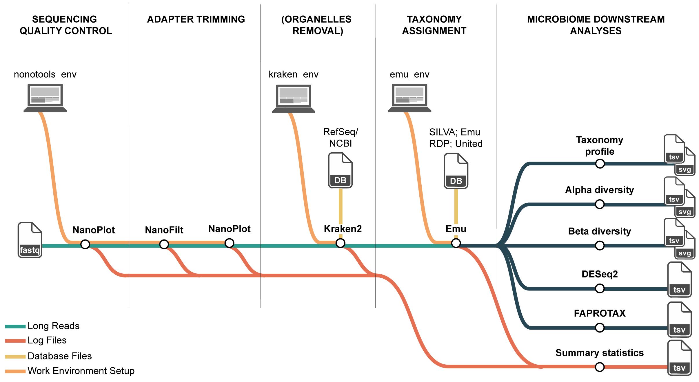
Overview of the long-read 16S rRNA microbiome workflow on high-performance computing (HPC). The pipeline comprises four steps and their primary inputs/outputs: (1) QC and filtering of Nanopore reads (NanoPlot, NanoFilt) producing per-sample QC reports and filtered FASTQ; (2) organelle removal with Kraken2 against a curated Viridiplantae (plastid and mitochondrial) database, yielding organelle-depleted FASTQ; (3) taxonomic assignment with Emu, generating four outputs, of which the species-level relative abundance table and the per-taxon read count table are used downstream; and (4) downstream ecological analyses that compute composition summaries and diversity metrics from these tables. Conda environments ensure reproducible tool execution on HPC, and log files from each step are retained for statistical summaries.
Background
Microbiomes play a central role in maintaining soil health and supporting plant development, influencing nutrient cycling, disease resistance, and overall ecosystem stability [1,2]. In both agricultural and natural systems, diverse microbial communities dominated by bacteria in soils and plant tissues are key drivers of biogeochemical processes such as carbon sequestration and nitrogen transformation [3]. Understanding the composition and functions of microbial communities provides a foundation for the development of new technologies, a guide for ecological management decisions, and the improvement of agricultural practices. However, accurate and consistent microbiome profiling remains a technical challenge, especially when dealing with complex environmental samples such as soil samples [4].
For bacterial community profiling, amplicon sequencing of the 16S rRNA gene remains a widely used, cost-effective approach for estimating community composition and diversity across environmental gradients and experimental manipulations [5]. In soils and plant compartments (rhizosphere, endosphere, and phyllosphere), where communities are both diverse and uneven, the ability to resolve taxa at finer ranks (e.g., species and, where possible, strain) improves the interpretability of ecological patterns and the portability of findings across studies [6,7]. Methodological advances have progressively increased taxonomic resolution and reproducibility in amplicon workflows. Early pipelines grouped reads into operational taxonomic units (OTUs) at fixed similarity thresholds, which simplified analysis but conflated biological and technical variation. However, these methods often fall short in delivering species-level resolution and are prone to variability across pipelines and datasets [8,9].
The shift toward exact sequence-based approaches (e.g., amplicon sequence variants, ASVs) reduced clustering artifacts for short-read data, improving comparability across experiments [10]. More recently, long-read sequencing has enabled recovery of near full-length 16S rRNA genes, potentially improving species-level assignment, disambiguating closely related taxa, and stabilizing ecological inferences in complex communities [11,12]. However, leveraging full-length reads requires algorithms that can accommodate read length–specific error structures, model multi-mapping to reference databases, and estimate abundances without overinflating diversity [13]. Emu, a taxonomic profiling method based on expectation-maximization (EM) to resolve ambiguous long-read mappings, yields compositional estimates that aim to be both accurate and robust for long-read 16S rRNA datasets [14].
Despite these advances, environmental microbiome studies still face challenges related to reproducibility and scale [5,15]. Reported community differences can be sensitive to choices in primer sets, reference databases, quality filters, and classification parameters, complicating meta-analysis and the accumulation of knowledge [8]. Soil and plant microbiomes also impose heavy computational demands due to complex experimental designs, due to high richness and the need for deeper sequencing to capture rare taxa, which can strain local computing resources [16]. High-performance computing (HPC) environments address scalability but are often perceived as inaccessible to new users and can themselves be sources of variability when software stacks, dependencies, or job-scheduling constraints differ across clusters [17,18]. For long-read 16S rRNA specifically, the lack of shared, domain-tailored, and fully documented workflows that integrate Emu with transparent quality control and benchmarking makes it difficult to evaluate performance across soil and plant compartments and to reproduce results across independent laboratories.
Consequently, there is a practical and conceptual gap: we lack a standardized, open, and reproducible long-read 16S rRNA pipeline that (i) is expressly designed for soil and plant microbiome questions, (ii) operationalizes best practices for quality control and reference-based inference with Emu, and (iii) scales predictably on HPC while producing portable, versioned outputs for downstream ecological analysis. Existing tutorials often target short-read OTU/ASV workflows or provide minimal guidance on how to tune long read–specific steps (e.g., length/quality screening, handling mapping, and database curation) under realistic environmental complexity [5,8,19]. Moreover, reproducibility guidance typically emphasizes containerization or environment capture but stops short of demonstrating that end-to-end results remain stable across different HPC clusters, settings, or modest updates to reference databases, factors that commonly change across institutional environments [15]. For interdisciplinary audiences, these limitations hinder the translation of microbiome insights into real practice interventions or ecological theory because conclusions may be contingent on opaque computational choices.
To address this need, a reproducible Emu-based workflow is presented for soil and plant microbiome profiling, designed for HPC execution while remaining accessible to users with varying computational backgrounds. The workflow is organized into four steps: long-read 16S rRNA gene input validation, quality control suited to full-length reads, reference-informed taxonomic assignment with Emu, and standardized outputs for ecological analyses, each accompanied by versioned configurations and human-readable reports. Reproducibility is supported through declarative configuration files so that identical inputs produce consistent outputs across different clusters, and scalability is demonstrated.
Software and datasets
The complete set of databases, software tools, and custom scripts required to reproduce this workflow is listed in Table 1, along with version numbers, access information, and licensing details. All custom scripts are available in the public GitHub repository and archived on Zenodo (DOI: 10.5281/zenodo.17764933; release v1.0.2).
Table 1. Databases, software, and custom scripts required to run the full Emu-based 16S microbiome workflow
| Type | Software/dataset/resource | Version | Date | License | Access |
|---|---|---|---|---|---|
| Database | RefSeq (NCBI) Viridiplantae (mitochondria) | 1.1 | May, 2025 | Free | |
| Database | RefSeq (NCBI) Viridiplantae (plastid) | 3.1 | May, 2025 | Free | |
| Database | Emu prebuilt DB (OSF 56uf7) | v3.4.5 | May, 2023 | CC-BY | Free |
| Database | FAPROTAX database | v1.2.12 | May, 2025 | CC-BY | Free |
| Software 1 | NanoPlot | 1.44.1 | June, 2023 | GPL-3.0 | Free |
| Software 2 | NanoStat | 1.6.0 | June, 2023 | GPL-3.0 | Free |
| Software 3 | NanoFilt | 2.8.0 | June, 2023 | GPL-3.0 | Free |
| Software 4 | Kraken2 | v.1.0 | July, 2025 | MIT | Free |
| Software 5 | Emu | v3.5.1 | January, 2021 | MIT | Free |
| Software 6 | R (base) | v4.4.2 | October, 2025 | GLP v2 | Free |
| Software 7 | Python | v3.8.0 | October, 2019 | BSD open source | Free |
| Script 1 | run_nanoplot_barcode.slurm | 10.5281/zenodo. 17764933; v1.0.2 | November, 2025 | CC-BY | Free |
| Script 2 | run_nanofilt.slurm | 10.5281/zenodo. 17764933; v1.0.2 | November, 2025 | CC-BY | Free |
| Script 3 | run_QC_summary.py | 10.5281/zenodo. 17764933; v1.0.2 | November, 2025 | CC-BY | Free |
| Script 4 | download_plant_organelle_RefSeq_fastas.sh | 10.5281/zenodo. 17764933; v1.0.2 | November, 2025 | CC-BY | Free |
| Script 5 | kraken2_add_build_db.slurm | 10.5281/zenodo. 17764933; v1.0.2 | November, 2025 | CC-BY | Free |
| Script 6 | kraken2_classify_filter.slurm | 10.5281/zenodo. 17764933; v1.0.2 | November, 2025 | CC-BY | Free |
| Script 7 | remove_kraken2_organelle_reads.py | 10.5281/zenodo. 17764933; v1.0.2 | November, 2025 | CC-BY | Free |
| Script 8 | summarize_kraken2_reports.py | 10.5281/zenodo. 17764933; v1.0.2 | November, 2025 | CC-BY | Free |
| Script 9 | run_emu.slurm | 10.5281/zenodo. 17764933; v1.0.2 | November, 2025 | CC-BY | Free |
| Script 10 | collect_counts.py | 10.5281/zenodo. 17764933; v1.0.2 | November, 2025 | CC-BY | Free |
| Script 11 | relab_to_counts.py | 10.5281/zenodo. 17764933; v1.0.2 | November, 2025 | CC-BY | Free |
| Script 12 | downstream_microbiome.r | 10.5281/zenodo. 17764933; v1.0.2 | November, 2025 | CC-BY | Free |
| Script 13 | emu-to-faprotax.py | 10.5281/zenodo. 17764933; v1.0.2 | November, 2025 | CC-BY | Free |
| Script 14 | collapse_table.py | 10.5281/zenodo. 17764933; v1.0.2 | November, 2025 | CC-BY | Free |
Procedure
Part I. Before you begin
Before initiating the four steps, it is advisable to organize the computational environment, define analysis parameters, and outline the overall workflow (see GitHub repository: https://github.com/henrimdias/emu-microbiome-HPC). The graphical overview presents a flowchart of the Emu pipeline, tracing the path from demultiplexed raw Oxford Nanopore FASTQ files through quality control, organelle filtering, expectation-maximization taxonomic assignment, and downstream ecological analyses. The following sections detail the principal considerations and options required for smooth and reproducible execution of the protocol.
Note: This protocol focuses exclusively on the computational analysis of Oxford Nanopore 16S reads and begins at the stage of base-called, demultiplexed FASTQ files. Procedures for base calling and demultiplexing (e.g., using Dorado, https://github.com/nanoporetech/dorado), as well as wet-lab steps for DNA extraction, library preparation, and sequencing, are outside the scope of this protocol.
A. Set up a directory structure
1. Create the project in a high-performance working space (often named scratch or work) for large, input/output-heavy runs, and keep code, configs, and finalized outputs in persistent project storage (often named project, groups, or shared). The layout may be created manually or, preferably, cloned from the GitHub template with paths adjusted as needed.
git clone --depth 1 --filter=blob:none --sparse https://github.com/henrimdias/emu-microbiome-HPC.gitcd emu-microbiome-HPCgit sparse-checkout set emu_pipelineNote: Retention and backup policies for the working space vary by cluster; check the cluster site docs.
B. Create and manage Conda environments
1. Maintain separate environments (nanotools_env, preemu_env, emu_env, faprotax_env) to avoid software conflicts.
2. Create each environment from YAML files provided in the repository (on the HPC login node).
nanotools_env:
cd yml_filesconda env create -f nanotools_env.ymlconda activate nanotools_envpreemu_env:
cd yml_filesconda env create -f preemu_env.ymlconda activate preemu_envemu_env:
cd yml_filesconda env create -f emu_env.ymlconda activate emu_envfaprotax_env:
cd yml_filesconda env create -f faprotax_env.ymlconda activate faprotax_envNote: YAML files ensure convenience and reproducibility. Alternatively, each protocol step also includes a one-liner for installing only the required tools without using YAMLs. Both approaches are valid.
Note: If Miniconda is not available on the cluster, install a local copy in your home directory and use it in all subsequent SLURM jobs. For example, on the login node:
cd $HOMEwget https://repo.anaconda.com/miniconda/Miniconda3-latest-Linux-x86_64.shbash Miniconda3-latest-Linux-x86_64.sh -b -p $HOME/miniconda3source $HOME/miniconda3/etc/profile.d/conda.shconda init bash # optionalAfter installation, make sure all SLURM scripts load this installation, e.g.:source $HOME/miniconda3/etc/profile.d/conda.shconda activate <env_name> C. Configure SLURM array jobs
Configure these settings in all SLURM files for each module, as illustrated in step A3 from Part II.
1. Use array indexing (e.g., --array=1-N) to parallelize per-sample steps.
2. Adjust memory (e.g., --mem=4G-24G) and CPU cores (e.g., --cpus-per-task=1-8) according to the demands of each tool (see Part I, section E).
3. Choose the recommended partition following the cluster policies (e.g., --partition=compute).
4. Change the directories following the recommended paths.
5. If Miniconda is not available, install it (e.g., in $HOME/miniconda3) and use this path as the source directory in all SLURM job scripts.
D. Reference databases
1. Select a reference database and fix its version to ensure stable and reproducible taxonomic assignments.
2. Record the database name, version, download date, source/DOI, and checksum.
3. By default, run the protocol with the Emu prebuilt database (OSF project 56uf7).
4. When customization is necessary, rebuild an Emu database from a pinned NCBI taxonomy following the Emu documentation: https://github.com/treangenlab/emu.
Note: A summary of widely used 16S rRNA gene reference databases, their most recent releases, and Emu-specific considerations to guide selection and version pinning is available in Table 2.
Caution: As new releases add sequences or rename taxa, identical reads may be classified differently. Version pinning avoids inconsistencies across runs.
Table 2. Common 16S rRNA gene reference options for Emu workflows
| Database | Scope/source | Latest release (version and date) | Notes for Emu | Reference |
|---|---|---|---|---|
| Emu prebuilt (OSF 56uf7) | Curated 16S bundle for Emu (NCBI/RefSeq) | OSF item “emu_default.tar.gz” last modified Mar 13, 2023 | Ready-to-use | [14] |
| SILVA SSU | Broad rRNA (SSU/LSU) curation | 138.2, Jul 11, 2024 | Custom Emu build required; SILVA v138.1 ready-to-use | [20] |
| Greengenes2 | Genome-informed reference tree and taxonomy | 2024.09, Oct 8, 2024 | Custom Emu build required | [21] |
| RDP | Classical 16S taxonomy/training data | Trainset 19, Jul 2023 | Custom Emu build required; RDPv11.5 ready-to-use | [22] |
| GTDB (R226) | Genome-based taxonomy with 16S representatives | R226, Apr 16, 2025 | Custom Emu build required | [23] |
E. Hardware preparation
The amount of RAM required depends on the dataset size and the complexity of the analysis. For the workflow described, which involves moderately complex steps, 16 GB of RAM is sufficient (Table 3).
Table 3. Recommended hardware and scheduler settings for each module of the workflow
| Module/step | Typical use case (as validated here) | Recommended CPUs and RAM (per task) | Example SLURM directives | Typical walltime (for ~18 samples) |
|---|---|---|---|---|
| QC and filtering of Nanopore reads | Full-length 16S Nanopore reads; 6 demultiplexed FASTQ files | 4 CPUs, 16 GB RAM | #SBATCH --partition=moderate* #SBATCH --cpus-per-task=4 #SBATCH --mem=16G #SBATCH --time=02:00:00 | ~20–40 min |
| Organelle database build (Kraken2) | Build Viridiplantae chloroplast + mitochondria Kraken2 database | 16 CPUs, 32–64 GB RAM | #SBATCH --partition=moderate* #SBATCH --cpus-per-task=16 #SBATCH --mem=32G #SBATCH --time=04:00:00 | ~60–120 min |
| Organelle classification and read filtering | Classify and remove organelle reads from 6 FASTQ files | 8 CPUs, 16 GB RAM per array task | #SBATCH --partition=moderate* #SBATCH --array=1-18 #SBATCH --cpus-per-task=8 #SBATCH --mem=16G #SBATCH --time=02:00:00 | ~30–60 min total |
| Taxonomic assignment with Emu | Emu profiling of organelle-depleted full-length 16S reads | 8 CPUs, 16 GB RAM per array task | #SBATCH --partition=moderate* #SBATCH --array=1-18 #SBATCH --cpus-per-task=8 #SBATCH --mem=16G #SBATCH --time=04:00:00 | ~30–60 min total |
| Downstream community and functional analyses | Alpha/beta diversity, ordination, DESeq2, FAPROTAX | 4 CPUs, 16 GB RAM | #SBATCH --partition=moderate* #SBATCH --cpus-per-task=4 #SBATCH --mem=16G #SBATCH --time=02:00:00 | ~30–90 min |
Note: Partition names (e.g., --partition=moderate) are cluster-specific and may differ across HPC systems. The settings shown here correspond to the compute infrastructure of the SDSU HPC and should be adapted to the partitions and resource limits available on other clusters.
For reference, check https://help.sdstate.edu/TDClient/2744/Portal/KB/ArticleDet?ID=159685.
F. Controls
Controls must span the entire workflow, not only the experimental design. Include extraction blanks and no-template PCR controls and process them through filtering, organelle depletion, taxonomic assignment, and downstream analyses; use at least one positive control (mock community) to benchmark length/quality thresholds and expected taxonomic recovery. Use blanks to identify contaminant taxa (e.g., blank-prevalent features) and to set acceptance ranges; report control outcomes with the main results and retain raw control tables for auditing. These practices are essential for low-biomass contexts and to avoid reagent/kit contaminants driving patterns (for a review, see [24]).
Part II. Preprocessing full-length 16S rRNA reads
This workflow performs automated quality control and filtering of full-length 16S rRNA Nanopore reads using a single SLURM pipeline that integrates NanoPlot, NanoFilt, and QC summary consolidation. The unified design minimizes manual editing by requiring only one configuration update at the top of the SLURM file before execution.
Timing: ~30 min (based on 18 .fastq files ranging between 150 and 220 MB).
Minimum disk space: ~8 GB.
A. Launch the unified nanotools pipeline
1. Ensure that all base-called, demultiplexed FASTQ files are placed in the raw-reads directory (e.g., emu_pipeline/raw_data) and follow a consistent naming pattern, such as barcodeXX.fastq.gz (for example, barcode01.fastq.gz, barcode02.fastq.gz) or user-defined sampleID.fastq.gz names that match the sample identifiers in the metadata table. The SLURM array scripts parse these filenames to derive sample IDs and map them to metadata.
2. Activate the Conda environment.
conda activate nanotools_env3. Open the SLURM file run_nanotools_pipeline.slurm and edit only the configuration section at the top of the file. Specify desired directories for raw reads, filtered reads, QC reports, and summary outputs:
# Example configuration block
RAW_DIR="/scratch/project/raw"FILTERED_DIR="/scratch/project/filtered"QC_DIR="/scratch/project/qc"SUMMARY_DIR="/scratch/project/summary"SCRIPT_QC_SUMMARY="/home/user/scripts/run_QC_summary.py"# Filtering parameters
MIN_LEN=1000MAX_LEN=1850MIN_QUAL=10Note: The script automatically detects files with extensions .fastq or .fastq.gz. There is no need to modify the file search pattern manually.
4. Submit the SLURM job to run the entire workflow.
sbatch run_nanotools_pipeline.slurmNote: This single command executes the following steps sequentially:
(i) NanoPlot: generates per-sample quality control (QC) reports for raw reads.
(ii) NanoFilt: filter reads by quality and length thresholds.
(iii) NanoPlot (filtered): regenerates QC reports after filtering.
(iv) QC summary: consolidates NanoStat metrics across samples and stages.
B. Filtering logic and parameters
Reads are filtered to 1,000–1,850 bp (Q ≥ 10) to enrich for full-length 16S rRNA gene amplicons (~1,450–1,600 bp) and exclude truncated (≤1,000 bp) and concatemeric or anomalously long (≥1,850 bp) reads, improving classification accuracy and comparability [25].
Expected outputs:
(i) Filtered FASTQ files (*_filtered.fastq.gz)
(ii) NanoPlot QC directories (/nanoplot_reports/raw and /nanoplot_reports/filtered)
(iii) Intermediate NanoStat summaries
C. Consolidating and visualizing QC reports
After the pipeline completes, the QC summary script automatically collects all NanoStat reports (raw and filtered) and merges them into an integrated summary.
If needed, the script can be run independently:
python run_QC_summary.py –-inpunt /put_the_directory –output /put_the_directoryExpected outputs:
(i) sequencing_summary.csv: Tables of all key NanoStat metrics (mean read length, quality, read count, N50, etc.).
(ii) QC_summary_plots.pdf: Multi-page PDF showing side-by-side comparisons (raw vs. filtered) per sample.
D. Quality verification and acceptance criteria
1. Confirm that read-length N50 values fall within the expected amplicon range (1,450–1,550 bp).
2. Ensure that read retention after filtering is between 60% and 90%.
3. Examine QC plots to confirm that the filtering step reduces truncated reads without excessive loss of valid reads.
Note: If results deviate (e.g., severe loss or unexpected quality shifts), adjust the parameters (MIN_LEN, MAX_LEN, or MIN_QUAL) in the configuration section of run_nanotools_pipeline.slurm and resubmit the job. See Table 2 for troubleshooting guidance if acceptance criteria are not met.
Caution: After filtering, the QC reports should show a controlled reduction in total read count and a reshaped quality/length distribution that reflects the chosen thresholds. If results deviate (e.g., abrupt read loss), adjust the parameters in run_nanofilt_barcodes.slurm.
Part III. Organelle contamination removal
Detect and remove organelle (chloroplast and mitochondrial) contamination from full-length Nanopore 16S rRNA reads. This step preserves accurate bacterial and archaeal community profiles for downstream Emu-based taxonomic analysis by eliminating host-derived organelle sequences. Reads are classified with Kraken2 [26] against a curated organelle reference database [27], and organelle-assigned reads are discarded. The result is a high-confidence, organelle-free read set for Emu, improving accuracy and reproducibility in plant and soil microbiome studies.
Timing: ~30–60 min (based on 18 .fastq files ranging between 150 and 220 MB).
Minimum disk space: ~12 GB.
A. Download curated RefSeq organelle genomes
1. Download curated chloroplast and mitochondrial FASTA files to construct the Kraken2 database. Run the organelle genome download script. Update and check pathways on the script before running the code.
bash download_plant_organelle_RefSeq_fastas.sh2. Verify downloaded and decompressed files.
ls -lh /$USER/scratch/emu_pipeline/kraken_db/Note: These files are multi-genome FASTAs curated by NCBI containing a wide range of plastid and mitochondrial sequences from green plants (May 2025 release).
B. Build the organelle database with Kraken2
1. Activate the Conda environment.
conda activate preemu_env2. Download taxonomy files.
kraken2-build --download-taxonomy –-db \/$USER/scratch/kraken_env/db/kraken_organelle_db3. Build the database with curated references using SLURM. Construct a Kraken2 organelle database from the curated RefSeq chloroplast and mitochondrial FASTA files downloaded in the previous step.
sbatch kraken2_add_build_db.slurmExpected database files: hash.k2d; opts.k2d; taxo.k2d; seqid2taxid.map.
C. Identify and filter organelle contamination
1. Use this database to classify reads and remove organelle-derived sequences from environmental full-length 16S rRNA gene datasets. The provided script applies Kraken2 using the default nucleotide parameters (k-mer length k = 35, minimizer length ℓ = 31, minimizer spaces s = 7), with a conservative confidence threshold of --confidence 0.6 [28]. Run the provided SLURM script:
sbatch kraken2_classify_filter.slurm2. Summarize contamination levels.
python summarize_kraken2_reports.py \ --input_dir /path/to/reports/ \ --output_file /path/to/output/kraken_contamination_summary.tsvExpected outputs: Per-sample classification outputs: *.kraken, *.report.txt; Organelle-depleted reads: *.fastq.gz; kraken_contamination_summary.tsv.
3. After depletion, confirm that bacterial reads dominate root libraries [29]. Check that organelle contamination does not exceed 15%–20% of classified reads.
4. Verify that the reads loss after filtering does not exceed 30%. Check code description in:
remove_kraken2_organelle_reads.py.5. Confirm that database provenance checks complete without errors, checking that report files are not empty or abnormal.
Note: Empty or abnormal report.txt files, unusually high organelle reads, or sharp bacterial losses (>30%) indicate potential database mismatch, over-filtering, or contamination. See Table 6 (Troubleshooting) for likely causes and corrective actions.
Part IV. Taxonomic assignment using Emu
Timing: ~30–60 min (based on 18 .fastq files ranging between 150 and 220 MB).
Minimum disk space: ~2 GB.
A. Prepare the Emu database
1. Download the prebuilt Emu database from OSF (https://osf.io/56uf7/) and set the directory path.
Note: The prebuilt Emu database requires approximately 90 MB of disk space.
2. Alternatively, build a custom database following the Emu GitHub instructions (https://github.com/treangenlab/emu; see Table 1) [30].
B. Run Emu with SLURM batch arrays
1. Inside the run_emu.slurm script, each array task calls Emu using a template command such as:
# -----------------------------------# 6. Run EMU abundance profiling# -----------------------------------echo "Running EMU on: $FASTA_FILE"emu abundance \ --db "$EMU_DB_DIR" \ --output-dir "$BARCODE_OUTPUT" \ --keep-counts \ --keep-read-assignments \ "$FASTA_FILE"Note: Here, EMU_DB_DIR points to the prebuilt Emu database (see Part IV, section A), FASTA_FILE is the organelle-depleted full-length 16S rRNA gene file for a given barcode, and BARCODE_OUTPUT is a per-sample directory where Emu writes relative abundance tables (*_rel-abundance.tsv) and read assignment distributions (*_read-assignment-distributions.tsv). It does not apply an additional minimum read-length filter inside Emu because length filtering to 1,000–1,850 bp (Q ≥ 10) is already enforced upstream with NanoFilt.
2. Activate the Conda environment.
conda activate emu_env3. Before running the job, confirm that the input directory contains organelle-depleted FASTQ files from the previous step, the Emu database is downloaded and indexed, and all directory paths in the SLURM script match the HPC environment.
4. Submit the SLURM job script:
sbatch run_emu.slurm5. Monitor the job array to confirm that each sample (barcode) runs as an independent task.
6. Typically, >95% of mapped reads should be assigned to a bacteria taxon.
Expected outputs: *_rel-abundance.tsv (taxa-level relative abundances); *_read-assignment-distributions.tsv (read-level mapping details).
C. Combine per-sample taxonomic tables
1. Merge all per-sample outputs into a single wide-format abundance table using the combine-outputs command:
emu combine-outputs <directory_path> <rank> Expected outputs: Combined abundance table (e.g., species_rel-abundance.tsv)
Note: This function generates a single table that contains the relative abundances of all Emu output files within a specified directory. It automatically selects all .tsv files in the directory that contain “rel-abundance” in their filename. It is also possible to combine tables at a specific taxonomic rank by specifying one of the following: tax_id, species, genus, family, order, class, phylum, or superkingdom. For more details, visit the GitHub repository: https://github.com/treangenlab/emu.
Caution: Regarding Emu, the quality of taxonomic assignment is evaluated based on the proportion of classified reads and the performance of controls. For example, in complex soils, low read assignment may indicate high error rates or gaps in the database rather than true biological absence [31]. If Emu fails to complete, expected output tables are missing, assignment rates are unexpectedly low at the genus or species level, array indexing skips or mislabels samples, or database paths/provenance are incorrect, consult the troubleshooting guidance for likely causes and corrective actions (see Table 6).
D. Aggregate Emu read-count statistics
1. After Emu completes, collect .out files generated per barcode (e.g., barcode01.out) that report three fields: Unmapped_Read_Count, Mapped_Read_Count, and Unclassified_Mapped_Read_Count. Place all .out files in a single directory.
2. Aggregate these counts across barcodes into one table using the provided script:
python collect_counts.py /path/to/directory3. Convert relative abundances into estimated raw read counts per barcode using the following script:
python relab_to_counts.py summary_counts.tsv relative_abundance.tsv raw_counts.tsv --strict-sumNote: Diversity indices that require integer counts (e.g., Chao1, rarefaction, DESeq2) must use these derived counts, not proportions.
Part V. Microbiome downstream analyses
Timing: ~60–120 min (based on 18 samples).
Minimum disk space: ~4 GB.
In the final stage of the workflow, downstream microbial community analysis is carried out in R, drawing on established ecological tools such as the vegan package [32]. Abundance tables and metadata provide the foundation for exploring sequencing depth, diversity, and community structure. Analyses typically include rarefaction curves, alpha diversity indices (e.g., Shannon, Simpson, Pielou’s evenness, Chao1), and beta diversity ordinations such as PCoA on Bray–Curtis dissimilarities. Differential abundance analysis can be performed with DESeq2 [33] using its internal size-factor normalization and false discovery rate (FDR)-adjusted P-values to identify taxa that change significantly across experimental groups. These are complemented by visualizations of taxonomic composition across selected ranks, while functional insights can be inferred with FAPROTAX [34]. Together, these approaches offer a flexible framework that can be readily adapted to a wide range of experimental designs. Table 4 summarizes the R version and core packages, together with their version numbers and roles in the workflow.
Table 4. R environment and packages used for microbiome downstream analyses
| Package | Version | Role in downstream workflow |
|---|---|---|
| data.table | 1.15.4 | Fast import/export of metadata, count tables, distance matrices, and diagnostic CSV files. |
| dplyr | 1.1.4 | Data wrangling for metadata and abundance tables, grouping and summarizing for plots and statistics. |
| tidyr | 1.3.1 | Reshaping tables for taxonomic composition plots and diversity summaries. |
| forcats | 1.0.1 | Factor management (ordering and relabeling groups and taxa for consistent plotting). |
| ggplot2 | 1.15.4 | Core plotting engine for rarefaction curves, composition barplots, alpha and beta diversity visualizations. |
| ggrepel | 0.9.5 | Non-overlapping sample labels in PCoA and NMDS plots. |
| ggpubr | 0.6.0 | Statistical annotations on alpha diversity boxplots (global tests, pairwise comparisons, significance labels). |
| vegan | 2.7.1 | Ecological analyses: rarefaction (rarefy), diversity indices, distance matrices (Bray, Jaccard), ordinations (NMDS), PERMANOVA, and betadisper. |
| rstatix | 0.7.2 | Assumption testing (Shapiro, Levene), ANOVA/Kruskal–Wallis, and post-hoc tests (Tukey/Dunn) for alpha diversity. |
| broom | 1.0.5 | Tidy summaries of model outputs (e.g., ANOVA tables) for export to CSV. |
| stringr | 1.5.1 | String manipulation and cleaning of labels where needed. |
| svglite | 2.1.3 | High-quality SVG export for all figures (used by save_plot_multi). |
| ape | 5.8 | PCoA with Cailliez correction as a robust fallback when cmdscale fails; phylogenetic utilities. |
Note: The downstream R script expects two main input tables:
(i) Metadata table (metadata.tsv): tab-delimited, with one row per sample and at least the following columns:
• SampleID (unique sample identifier; must match column names in the count table).
• Group (experimental group or treatment).
(ii) Count table (counts.tsv): tab-delimited matrix with the following:
• One row per taxon (e.g., species or genus).
• One column per sample (SampleID).
• An initial column with Taxon (or Species) storing the taxonomic label.
(iii) Relative abundance table (relative_counts.tsv): same structure as the count table, but with remaining cells containing relative abundances (e.g., output from Emu pipeline) instead of raw counts.
An example dataset (example_metadata.tsv, example_counts.tsv) that satisfies these requirements is provided in the GitHub repository (under emu_pipeline/example_data/) and in the Zenodo archive. Users can run the full downstream script on this example dataset to verify that their installation and configuration are working before analyzing their own data.
A. Run the downstream analysis workflow in R
1. Download downstream_microbiome.R from the repository.
2. Open and edit the configuration block at the top of the script: set metadata_path, raw_counts_path, rel_abund_path, and EXPORT_DIR. Confirm sample_id_col, group_col, and tax_level match the metadata table.
# ============================================================# 1) User configuration (edit for a given dataset)# ============================================================# Path to metadata table (one row per sample)metadata_path <- "metadata.tsv"# Path to raw count table (features in rows, samples in columns)raw_counts_path <- "raw_counts.tsv"# Path to relative abundance tablerel_abund_path <- "raw_counts.tsv"# Column name in metadata containing sample IDssample_id_col <- "SampleID"# Column name used as the main grouping factor (for colors / statistics)group_col <- "Group"# Target taxonomic rank for composition plots (case-insensitive).# Typical choices: "kingdom", "phylum", "class", "order", "family", "genus", "species".tax_level <- "genus"# Number of most abundant taxa to display explicitly in composition plotstopN_taxa <- 16# Number of interpolation steps for rarefaction curvesraref_steps <- 100# Output directory for all plots and tablesEXPORT_DIR <- "downstream_microbiome_output"dir.create(EXPORT_DIR, showWarnings = FALSE, recursive = TRUE)# Optional: preprocessing for alpha diversity (filters / rarefaction on raw counts)filter_for_alpha <- FALSE # if TRUE, apply filters below (must be used for Chaos1)min_lib_alpha <- 1000 # minimum reads per sample for alpha analysesmin_prevalence <- 2 # minimum number of samples in which a feature must be presentmin_total_count <- 10 # minimum total counts per feature (across all samples)rarefy_for_alpha <- FALSE # if TRUE, perform rarefaction for alpha analysesrare_depth_alpha <- NA # if NA, uses minimum library size after filtering# Optional: minimum library size for inclusion in beta diversitymin_lib_beta <- 1 # 1 removes only zero-library samples3. Run the script locally in RStudio or from the command line:
Rscript downstream_microbiome.RExpected outputs: PNG/SVG figures (rarefaction, composition bar charts, alpha diversity, PCoA/NMDS) and CSV tables (alpha metrics, PERMANOVA/betadisper results, DESeq2 outputs).
Note: The script is fully commented to support customization and guides users through a complete downstream workflow, including rarefaction curves for sequencing depth assessment, taxonomic composition plots at chosen ranks, alpha diversity metrics (S_obs, Chao1, Shannon, Simpson, Pielou’s evenness), beta diversity ordinations (Bray, Jaccard, Aitchison with PCoA/NMDS), PERMANOVA and dispersion testing (betadisper), and differential abundance analysis with DESeq2 using size-factor normalization and FDR-adjusted results.
B. Assign putative functions with FAPROTAX
1. Download the FAPROTAX database (v1.2.12, last updated May 2025; [34]) from: http://www.loucalab.com/archive/FAPROTAX/lib/php/index.php?section=Download
2. Activate the Conda environment.
conda activate faprotax_env3. Prepare the input table with taxonomy, sample IDs, and counts/abundances. Convert Emu outputs using:
python emu-to-faprotax.py relative_abundance.tsv faprotax_relative_abundance.tsv4. Run FAPROTAX in tabular mode to generate function-by-sample profiles:
python collapse_table.py \-i faprotax_relative_abundance.tsv \-o func_faprotax_relative_abundance.tsv \-g FAPROTAX.txt -d "taxonomy" -c "#" -vExpected outputs: func_faprotax_relative_abundance.tsv (function-by-sample matrix).
Note: FAPROTAX accuracy depends on the quality of taxonomic assignments. Misclassifications at the genus/species level may propagate into functional predictions.
Validation of protocol
This protocol has been used and validated in Dias et al. [35]. The study applied the workflow to full-length 16S rRNA Nanopore datasets from seasonal yellow pea varieties, demonstrating organelle read removal, Emu-based taxonomic assignment, and downstream ecological analyses. Detailed results are presented in Figure 2 (alpha diversity metrics) and Figure 4 (community composition profiles) of [35].
General notes and troubleshooting
Before inspecting module-specific issues, it is recommended that users perform a few high-level checks on read retention, organelle removal, taxonomic assignment rates, and diversity-ready sampling depth. Table 5 summarizes indicative sanity-check thresholds based on the validation dataset.
Table 5. Quick sanity-check thresholds across the workflow
| Workflow step | Metric | Indicative threshold (validation dataset) | How to check |
|---|---|---|---|
| QC and NanoFilt filtering | Post-NanoFilt read retention | ≥70%–80% of reads retained after quality and length filtering | Compare total reads before and after NanoFilt using NanoStat summaries or per-sample FASTQ statistics. Large losses may indicate overly stringent filters or poor runs. |
| Organelle removal (Kraken2) | Organelle contamination (before/after) | Initial organelle fraction often ~5%–40%; after Kraken2 filtering, residual organelle reads should be <1% | Use kraken2 reports or summarize_kraken2_reports.py to compute the proportion of organelle-assigned reads pre- and post-filtering. |
| Taxonomic assignment (Emu) | Classification/mapping rates | ≥70% of reads mapped to the Emu database and ≥60% assigned at least to the genus level for high-quality runs | Inspect Emu summary outputs for per-sample mapping and classification rates; low values may indicate database gaps or poor read quality rather than true absence. |
| Input depth for diversity | Minimum counts per sample + rarefaction | Samples with <5,000–10,000 16S rRNA reads after filtering and strongly non-saturating rarefaction curves should be treated cautiously or excluded from alpha/beta analyses | Use the downstream R script to (i) inspect per-sample read counts and (ii) inspect rarefaction curves: samples whose curves do not approach a plateau at the chosen depth likely have insufficient coverage. |
| Beta diversity and PERMANOVA | Dispersion vs. group centroids | Significant heterogeneity of dispersion (betadisper p < 0.05) implies PERMANOVA results must be interpreted with caution | Examine vegan::betadisper and its permutation test (permutest) alongside PERMANOVA (adonis2); unequal dispersion can drive apparent group separation. |
Common problems, their likely causes, and practical solutions are summarized in Table 6. This table covers issues that arise across the pipeline, including key references.
Table 6. Common pitfalls in microbiome analysis: quick diagnostics and solutions
| Nature | Problem | Possible cause | Solution | Key references |
|---|---|---|---|---|
| Experimental | No plateau in rarefaction | Insufficient sequencing depth; highly uneven communities | Increase sequencing depth or pool runs or use coverage-based comparisons; reserve rarefaction for QC. | [36] |
| Statistical | Rarefaction curves with irregular “kinks” | Residual chimeras/contaminants; batch effects | Apply contaminant/chimera filtering; evaluate batch effects; remove outlier samples if justified. | [37] |
| Statistical | Comparing groups at minimum depth drops many samples | The minimum read threshold excludes many libraries | Use a higher common coverage rather than the minimum; report sensitivity analyses (e.g., 50k vs. 100k reads). | [38] |
| Statistical | Rarefaction used as normalization for differential abundance | Methodological misuse | Use size-factor or compositional methods (e.g., DESeq2); limit rarefaction to alpha/QC. | [39] |
| Statistical | PERMANOVA significant with unequal dispersion | Group dispersions differ | Test dispersion; report heterogeneity; consider constrained permutations; interpret with caution. | [40] |
| Statistical | PERMANOVA significant, but little 2D separation | Separation occurs on higher axes; low variance on PC1/PC2 | Inspect additional axes; provide scree/cumulative variance; consider covariates. | [40] |
| Statistical | High NMDS stress (≥0.2) | Weak signal; inappropriate distance; sparsity | Try alternative distances (Bray/Jaccard/Aitchison); increase dimensionality k; filter low-prevalence features. | [41] |
| Statistical | NMDS stress ≈ 0 with warnings | Duplicate or near-identical samples | Check for duplicates/zero variance; remove true duplicates; mitigate label overlap. | [41] |
| Statistical | Chao1 inflated or NA | Many singletons; excess zeros | Compute from raw counts; consider coverage-based richness and report confidence intervals. | [42] |
| Statistical | Chao1 behaves erratically | Using relative abundances; many singletons | Compute Chao1 from raw counts only; consider coverage-based richness if necessary. | |
| Methods | Bray calculated on raw counts | Library-size confounding | Convert to per-sample proportions (relative abundance) prior to Bray–Curtis. | [43] |
| Method | Jaccard misses abundance patterns | Presence/absence only | Prefer Bray or Aitchison when abundance magnitudes are relevant; justify the metric choice. | [44] |
| Method | Aitchison fails with zeros | Structural zeros in compositions | Apply a small pseudo-count or multiplicative replacement; perform sensitivity analysis on pseudo-count. | [44] |
| Method | Negative eigenvalues in PCoA | Non-Euclidean distances | Use eigenvalue corrections or methods that handle non-Euclidean metrics. | |
| Method | Rank mismatch in composition plots | Relative table with a different taxonomic rank | Re-aggregate to the chosen rank and re-normalize per sample; document the final rank used. | |
| Method | Unexpected drop in bacterial reads after organelle filtering | Over-filtering due to DB/content mismatch | Spot-check read classifications; adjust thresholds; refine the organelle DB; re-run a subset. | |
| QC | Large read loss after filtering | Thresholds too strict; path mix-ups | Revisit quality/length cutoffs; verify input/output folders; confirm file naming and sample lists. | |
| QC | Pronounced batch/run effects | Extraction/kit/day effects | Include batch in models; use strata to restrict permutations. | |
| QC | Contaminants drive patterns | Incomplete decontamination | Include negative controls; remove known environmental contaminants; reprocess if needed. | [24,37] |
| QC | Extreme sparsity/zeros | Many rare features | Apply prevalence and total-count filters; report the proportion of features removed. | |
| QC | Sample ID mismatches | Inconsistent naming between metadata and matrices | Harmonize identifiers; log dropped/added samples; rerun checks before analysis. | |
| Design | Unbalanced group sizes | Inflated type I error; reduced power | Report sample sizes; use constrained permutations or covariates; consider stratified resampling. | [8] |
| Design | Too few replicates for ellipses | n < 3 per group | Omit ellipses; show centroids or convex hulls; note the limitation. | |
| Visualization | Overplotted labels | Many samples; short axes | Use label repulsion; facet by group; increase figure size; limit labels to selected points when appropriate. | |
| Computational | Long runtimes | Large matrices; slow ordination | Prefilter low-prevalence taxa; parallelize distance computation; cache ordination. | |
| Reproducibility | The results vary between runs | Random seeds; package versions | Set random seeds for NMDS and permutations; record software versions in the report. | |
| Interpretation | Only dispersion tests are significant | Difference in variability, not centroids | Report dispersion results; qualify the PERMANOVA interpretation accordingly. | [40] |
| Sensitivity | Results depend on filtering or pseudo-count | Threshold sensitivity | Report sensitivity across prevalence/abundance thresholds and pseudo-count settings; include a comparison table. |
Supplementary information
Supplementary materials are available with the online version of this article and in the associated GitHub repository (https://github.com/henrimdias/emu-microbiome-HPC). Supplementary data have been deposited in Zenodo (DOI: 10.5281/zenodo.17195104).
Acknowledgments
Authors’ contribution
Conceptualization, H.M.D. and C.G.; Investigation, H.M.D., R.J., and C.G.; Writing—Original Draft, H.M.D.; Writing—Review & Editing, H.M.D., R.J., V.A.S., J.L.G.H., S.S., H.M.M., and C.G.; Funding acquisition, S.S. and C.G.; Supervision, C.G.
Startup funding to the S.S. lab from the Agricultural Experiment Station (AES), SDSU. We thank Mehmet Karakaya for his unwavering support during late-night work sessions, generously providing food, humor, and care throughout the development of this protocol.
This protocol has been used and validated in Dias et al. [35].
Competing interests
The authors declare no conflict of interest.
References
- Hartmann, M. and Six, J. (2022). Soil structure and microbiome functions in agroecosystems. Nat Rev Earth Environ. 4(1): 4–18. https://doi.org/10.1038/s43017-022-00366-w
- Pantigoso, H. A., Newberger, D. and Vivanco, J. M. (2022). The rhizosphere microbiome: Plant–microbial interactions for resource acquisition. J Appl Microbiol. 133(5): 2864–2876. https://doi.org/10.1111/jam.15686
- Islam, W., Noman, A., Naveed, H., Huang, Z. and Chen, H. Y. H. (2020). Role of environmental factors in shaping the soil microbiome. Environ Sci Pollut Res. 27(33): 41225–41247. https://doi.org/10.1007/s11356-020-10471-2
- Liu, Y. X., Qin, Y., Chen, T., Lu, M., Qian, X., Guo, X. and Bai, Y. (2021). A practical guide to amplicon and metagenomic analysis of microbiome data. Protein Cell. 12(5): 315–330. https://doi.org/10.1007/s13238-020-00724-8
- Knight, R., Vrbanac, A., Taylor, B. C., Aksenov, A., Callewaert, C., Debelius, J., Gonzalez, A., Kosciolek, T., McCall, L.-I., McDonald, D., et al. (2018). Best practices for analysing microbiomes. Nat Rev Microbiol. 16(7): 410–422. https://doi.org/10.1038/s41579-018-0029-9
- Alteio, L. V., Séneca, J., Canarini, A., Angel, R., Jansa, J., Guseva, K., Kaiser, C., Richter, A. and Schmidt, H. (2021). A critical perspective on interpreting amplicon sequencing data in soil ecological research. Soil Biol Biochem. 160: 108357. https://doi.org/10.1016/j.soilbio.2021.108357
- Shade, A. and Handelsman, J. (2011). Beyond the Venn diagram: the hunt for a core microbiome. Environ Microbiol. 14(1): 4–12. https://doi.org/10.1111/j.1462-2920.2011.02585.x
- Abellan-Schneyder, I., Matchado, M. S., Reitmeier, S., Sommer, A., Sewald, Z., Baumbach, J., List, M. and Neuhaus, K. (2021). Primer, Pipelines, Parameters: Issues in 16S rRNA Gene Sequencing. mSphere. 6(1): e01202–20. https://doi.org/10.1128/msphere.01202-20
- Fasolo, A., Deb, S., Stevanato, P., Concheri, G. and Squartini, A. (2024). ASV vs OTUs clustering: Effects on alpha, beta, and gamma diversities in microbiome metabarcoding studies. PLoS One. 19(10): e0309065. https://doi.org/10.1371/journal.pone.0309065
- Callahan, B. J., McMurdie, P. J., Rosen, M. J., Han, A. W., Johnson, A. J. A. and Holmes, S. P. (2016). DADA2: High-resolution sample inference from Illumina amplicon data. Nat Methods. 13(7): 581–583. https://doi.org/10.1038/nmeth.3869
- Benítez-Páez, A. and Sanz, Y. (2017). Multi-locus and long amplicon sequencing approach to study microbial diversity at species level using the MinIONTM portable nanopore sequencer. GigaScience. 6(7): gix043. https://doi.org/10.1093/gigascience/gix043
- Karst, S. M., Ziels, R. M., Kirkegaard, R. H., Sørensen, E. A., McDonald, D., Zhu, Q., Knight, R. and Albertsen, M. (2021). High-accuracy long-read amplicon sequences using unique molecular identifiers with Nanopore or PacBio sequencing. Nat Methods. 18(2): 165–169. https://doi.org/10.1038/s41592-020-01041-y
- Alser, M., Rotman, J., Deshpande, D., Taraszka, K., Shi, H., Baykal, P. I., Yang, H. T., Xue, V., Knyazev, S., Singer, B. D., et al. (2021). Technology dictates algorithms: recent developments in read alignment. Genome Biol. 22(1): 249. https://doi.org/10.1186/s13059-021-02443-7
- Curry, K. D., Wang, Q., Nute, M. G., Tyshaieva, A., Reeves, E., Soriano, S., Wu, Q., Graeber, E., Finzer, P., Mendling, W., et al. (2022). Emu: species-level microbial community profiling of full-length 16S rRNA Oxford Nanopore sequencing data. Nat Methods. 19(7): 845–853. https://doi.org/10.1038/s41592-022-01520-4
- Kulkarni, N., Alessandrì, L., Panero, R., Arigoni, M., Olivero, M., Ferrero, G., Cordero, F., Beccuti, M. and Calogero, R. A. (2018). Reproducible bioinformatics project: a community for reproducible bioinformatics analysis pipelines. BMC Bioinf. 19(S10): 349. https://doi.org/10.1186/s12859-018-2296-x
- Zhou, J., He, Z., Yang, Y., Deng, Y., Tringe, S. G. and Alvarez-Cohen, L. (2015). High-Throughput Metagenomic Technologies for Complex Microbial Community Analysis: Open and Closed Formats. mBio. 6(1): e02288-14. https://doi.org/10.1128/mBio.02288-14
- Baichoo, S., Souilmi, Y., Panji, S., Botha, G., Meintjes, A., Hazelhurst, S., Bendou, H., Beste, E. d., Mpangase, P. T., Souiai, O., et al. (2018). Developing reproducible bioinformatics analysis workflows for heterogeneous computing environments to support African genomics. BMC Bioinf. 19(1): 457. https://doi.org/10.1186/s12859-018-2446-1
- Wilkinson, M. D., Dumontier, M., Aalbersberg, Ij. J., Appleton, G., Axton, M., Baak, A., Blomberg, N., Boiten, J.-W., Da Silva Santos, L. B., Bourne, P. E., et al. (2016). The FAIR Guiding Principles for scientific data management and stewardship. Sci Data. 3(1): 160018. https://doi.org/10.1038/sdata.2016.18
- Bharti, R. and Grimm, D. G. (2019). Current challenges and best-practice protocols for microbiome analysis. Briefings Bioinf. 22(1): 178–193. https://doi.org/10.1093/bib/bbz155
- Quast, C., Pruesse, E., Yilmaz, P., Gerken, J., Schweer, T., Yarza, P., Peplies, J. and Glöckner, F. O. (2012). The SILVA ribosomal RNA gene database project: improved data processing and web-based tools. Nucleic Acids Res. 41: D590–D596. https://doi.org/10.1093/nar/gks1219
- McDonald, D., Jiang, Y., Balaban, M., Cantrell, K., Zhu, Q., Gonzalez, A., Morton, J. T., Nicolaou, G., Parks, D. H., Karst, S. M., et al. (2024). Greengenes2 unifies microbial data in a single reference tree. Nat Biotechnol. 42(5): 715–718. https://doi.org/10.1038/s41587-023-01845-1
- Cole, J. R., Wang, Q., Fish, J. A., Chai, B., McGarrell, D. M., Sun, Y., Brown, C. T., Porras-Alfaro, A., Kuske, C. R., Tiedje, J. M., et al. (2013). Ribosomal Database Project: data and tools for high throughput rRNA analysis. Nucleic Acids Res. 42: D633–D642. https://doi.org/10.1093/nar/gkt1244
- Parks, D. H., Chuvochina, M., Rinke, C., Mussig, A. J., Chaumeil, P. A. and Hugenholtz, P. (2021). GTDB: an ongoing census of bacterial and archaeal diversity through a phylogenetically consistent, rank normalized and complete genome-based taxonomy. Nucleic Acids Res. 50: D785–D794. https://doi.org/10.1093/nar/gkab776
- Eisenhofer, R., Minich, J. J., Marotz, C., Cooper, A., Knight, R. and Weyrich, L. S. (2019). Contamination in Low Microbial Biomass Microbiome Studies: Issues and Recommendations. Trends Microbiol. 27(2): 105–117. https://doi.org/10.1016/j.tim.2018.11.003
- Butler, I., Turner, O., Mohammed, K., Akhtar, M., Evans, D., Lambourne, J., Harris, K., O'Sullivan, D. M. and Sergaki, C. (2025). Standardization of 16S rRNA gene sequencing using nanopore long read sequencing technology for clinical diagnosis of culture negative infections. Front Cell Infect Microbiol. 15: e1517208. https://doi.org/10.3389/fcimb.2025.1517208
- Wood, D. E., Lu, J. and Langmead, B. (2019). Improved metagenomic analysis with Kraken 2. Genome Biol. 20(1): 257. https://doi.org/10.1186/s13059-019-1891-0
- Goldfarb, T., Kodali, V. K., Pujar, S., Brover, V., Robbertse, B., Farrell, C. M., Oh, D. H., Astashyn, A., Ermolaeva, O., Haddad, D., et al. (2024). NCBI RefSeq: reference sequence standards through 25 years of curation and annotation. Nucleic Acids Res. 53: D243–D257. https://doi.org/10.1093/nar/gkae1038
- Liu, Y., Ghaffari, M. H., Ma, T. and Tu, Y. (2024). Impact of database choice and confidence score on the performance of taxonomic classification using Kraken2. aBIOTECH. 5(4): 465–475. https://doi.org/10.1007/s42994-024-00178-0
- Giangacomo, C., Mohseni, M., Kovar, L. and Wallace, J. G. (2021). Comparing DNA Extraction and 16S rRNA Gene Amplification Methods for Plant-Associated Bacterial Communities. Phytobiomes J. 5(2): 190–201. https://doi.org/10.1094/pbiomes-07-20-0055-r
- Curry, K. D., Soriano, S., Nute, M. G., Villapol, S., Dilthey, A. and Treangen, T. J. (2024). Microbial Community Profiling Protocol with Full‐length 16S rRNA Sequences and Emu. Curr Protocol. 4(3): e978. https://doi.org/10.1002/cpz1.978
- Wright, R. J., Comeau, A. M. and Langille, M. G. I. (2023). From defaults to databases: parameter and database choice dramatically impact the performance of metagenomic taxonomic classification tools. Microb Genomics. 9(3): e000949. https://doi.org/10.1099/mgen.0.000949
- Oksanen, J., Simpson, G. L., Blanchet, F. G., Kindt, R., Legendre, P., Minchin, P. R., O’Hara, R. B., Solymos, P., Stevens, M. H. H., Szoecs, E., et al. (2001). vegan: Community Ecology Package (p. 2.7-1). Data set. https://doi.org/10.32614/CRAN.package.vegan
- Love, M. I., Huber, W. and Anders, S. (2014). Moderated estimation of fold change and dispersion for RNA-seq data with DESeq2. Genome Biol. 15(12): 550. https://doi.org/10.1186/s13059-014-0550-8
- Louca, S., Parfrey, L. W. and Doebeli, M. (2016). Decoupling function and taxonomy in the global ocean microbiome. Science. 353(6305): 1272–1277. https://doi.org/10.1126/science.aaf4507
- Dias, H. M., Solanki, S., Gonzalez‐Hernandez, J. L., Mural, R. V., Yurgel, S. N. and Graham, C. (2025). Influence of Plant Genotype on Nodule‐Associated Bacterial Community Composition and Function in Seasonal Field Pea Varieties. Legume Sci. 7(4): e70069. https://doi.org/10.1002/leg3.70069
- Schloss, P. D. (2024). Rarefaction is currently the best approach to control for uneven sequencing effort in amplicon sequence analyses. mSphere. 9(2): e00354-23. https://doi.org/10.1128/msphere.00354-23
- Fierer, N., Leung, P. M., Lappan, R., Eisenhofer, R., Ricci, F., Holland, S. I., Dragone, N., Blackall, L. L., Dong, X., Dorador, C., et al. (2025). Guidelines for preventing and reporting contamination in low-biomass microbiome studies. Nat Microbiol. 10(7): 1570–1580. https://doi.org/10.1038/s41564-025-02035-2
- McKnight, D. T., Huerlimann, R., Bower, D. S., Schwarzkopf, L., Alford, R. A. and Zenger, K. R. (2019). Methods for normalizing microbiome data: An ecological perspective. Methods Ecol Evol. 10(3): 389–400. https://doi.org/10.1111/2041-210X.13115
- Xia, Y. (2023). Statistical normalization methods in microbiome data with application to microbiome cancer research. Gut Microbes. 15(2): e2244139. https://doi.org/10.1080/19490976.2023.2244139
- Regueira‐Iglesias, A., Balsa‐Castro, C., Blanco‐Pintos, T. and Tomás, I. (2023). Critical review of 16S rRNA gene sequencing workflow in microbiome studies: From primer selection to advanced data analysis. Mol Oral Microbiol. 38(5): 347–399. https://doi.org/10.1111/omi.12434
- Dexter, E., Rollwagen‐Bollens, G. and Bollens, S. M. (2018). The trouble with stress: A flexible method for the evaluation of nonmetric multidimensional scaling. Limnol Oceanogr Methods. 16(7): 434–443. https://doi.org/10.1002/lom3.10257
- Chiu, C. H. and Chao, A. (2016). Estimating and comparing microbial diversity in the presence of sequencing errors. PeerJ. 4: e1634. https://doi.org/10.7717/peerj.1634
- Weiss, S., Xu, Z. Z., Peddada, S., Amir, A., Bittinger, K., Gonzalez, A., Lozupone, C., Zaneveld, J. R., Vázquez-Baeza, Y., Birmingham, A., et al. (2017). Normalization and microbial differential abundance strategies depend upon data characteristics. Microbiome. 5(1): 27. https://doi.org/10.1186/s40168-017-0237-y
- Fuschi, A., Merlotti, A. and Remondini, D. (2025). Microbiome data: tell me which metrics and I will tell you which communities. ISME Commun. 5(1): e1093/ismeco/ycaf125. https://doi.org/10.1093/ismeco/ycaf125
Article Information
Publication history
Received: Sep 29, 2025
Accepted: Dec 7, 2025
Available online: Jan 4, 2026
Published: Jan 20, 2026
Copyright
© 2026 The Author(s); This is an open access article under the CC BY-NC license (https://creativecommons.org/licenses/by-nc/4.0/).
How to cite
Dias, H. M., Jain, R., Santos, V. A., Gonzalez-Hernandez, J. L., Solanki, S., Menendez III, H. M. and Graham, C. (2026). Reproducible Emu-Based Workflow for High-Fidelity Soil and Plant Microbiome Profiling on HPC Clusters. Bio-protocol 16(2): e5577. DOI: 10.21769/BioProtoc.5577.
Category
Bioinformatics and Computational Biology
Microbiology > Community analysis > Metagenomics
Plant Science > Plant immunity > Host-microbe interactions
Do you have any questions about this protocol?
Post your question to gather feedback from the community. We will also invite the authors of this article to respond.