- Protocols

- Articles and Issues
- For Authors
- About
- Become a Reviewer

Bridging PCR-Based Genome-Walking Protocol
Published: Vol 15, Iss 23, Dec 5, 2025 DOI: 10.21769/BioProtoc.5531 Views: 1036
Reviewed by: Anu ThomasAlberto RissoneAnonymous reviewer(s)
Original research article
The authors used this protocol in:
Jan 2023

Protocol Collections
Comprehensive collections of detailed, peer-reviewed protocols focusing on specific topics


Abstract
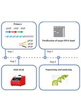
Genome walking is a classical molecular biology technique used to amplify unknown regions flanking known DNA sequences. Genome walking holds a vital position in the areas associated with molecular biology. However, existing genome-walking protocols still face issues in experimental operation or methodological specificity. Here, we propose a novel genome-walking protocol based on bridging PCR. The critical factor of this protocol is the use of a bridging primer, which is made by attaching an oligomer (or tail primer sequence) to the 5′ end of the walker primer 5′ region. When the bridging primer anneals to the walker primer site, this site will elongate along the tail of the bridging primer. The non-target product (the main contributor to background in genome walking), defined by the walker primer, is lengthened at both ends. In the next PCR(s), the annealing between the two lengthened ends is easier than the annealing between them and the shorter tail primer. As a result, this non-target product is eliminated without affecting target amplification.
Key features
• This bridging PCR protocol, built upon the technique developed by Lin et al. [1], is universal.
• The bridging primer is made by attaching a tail DNA to the 5′ end of the walker primer 5′ region.
• Lengthening of non-target DNA by both ends of bridging primer results in intrastrand annealing or hairpin formation, the basis for the removal of non-target background.
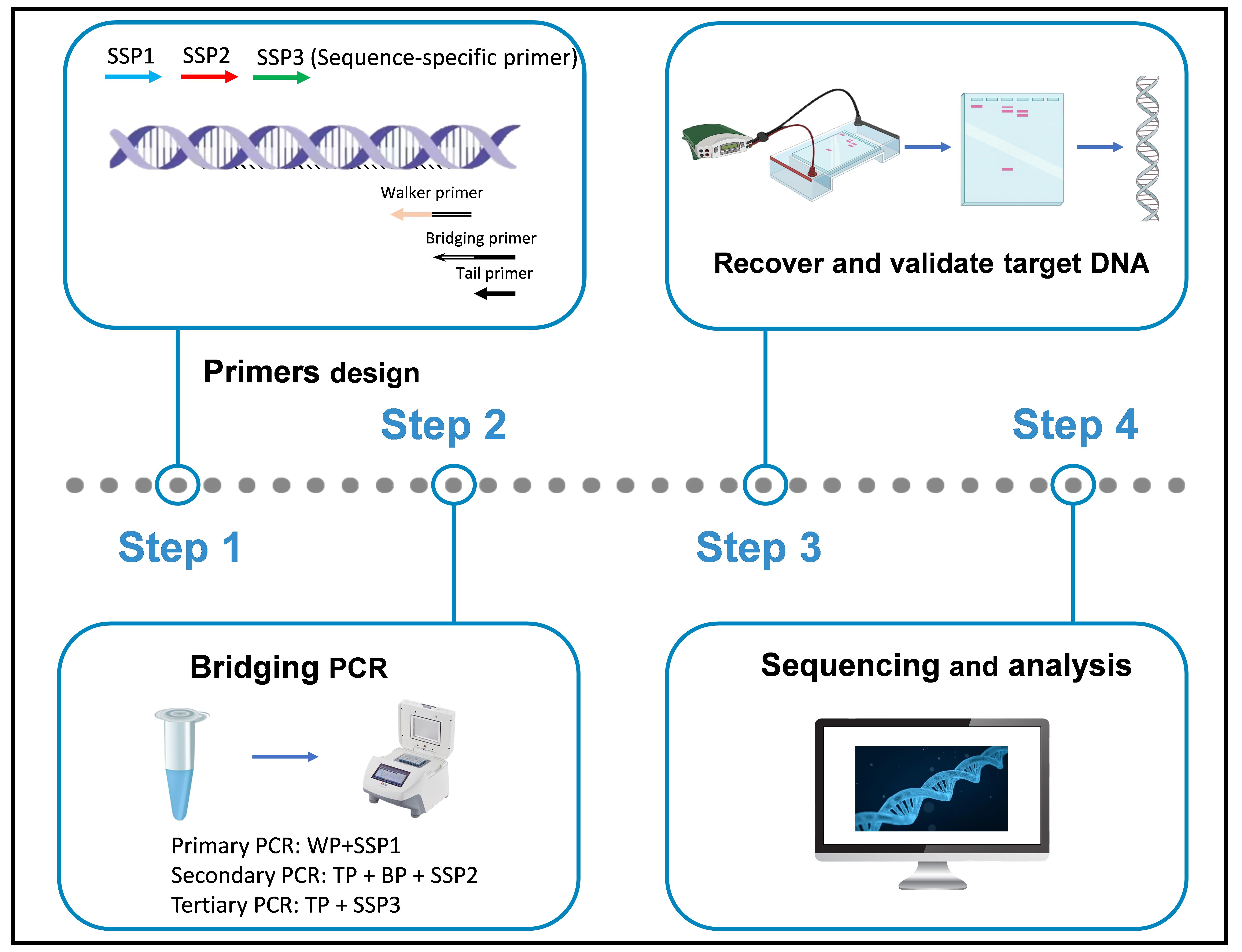
Keywords: Bridging PCRGraphical overview
Background
Genome walking (GW) is a molecular tool for cloning unknown regions flanking known DNAs, facilitating methods such as gene cloning, identifying DNA mutations, and analyzing transgenic sites [2–5]. Up to date, three types of GW were available: random PCRs, genome library-based techniques, and restriction-ligation-based PCRs. Among them, genome library-based techniques are time-consuming and inefficient, due to requiring the construction and screening of a genomic DNA library, and restriction-ligation-based PCRs require the digestion of genomic DNA and the subsequent ligation of the digested product prior to amplification. Comparatively, random PCRs are faster and more efficient, as the extra steps prior to amplification are omitted [6–10].
Random PCRs generally require two to three rounds of nested amplification. In primary amplification, a low-temperature annealing cycle allows the walking primer (WP) to randomly anneal to the unknown flank, thereby synthesizing a target DNA comprising a known region and its unknown flank. The following round or two of nested amplification further enrich this DNA, ultimately achieving the so-called genome walking [11–15]. However, due to the use of WP and at least one low-temperature cycle in each round of amplification, three types of non-target amplicons will be produced. Type I is synthesized by GSP alone; type II is synthesized by GSP and WP; and type III is synthesized by WP alone. Types I and II can be easily removed in the next PCR because they lack an authentic binding site for the sequence-specific primer (SSP). The real challenge is how to eliminate the type III non-target product [16–19]. Existing random PCRs, such as thermal asymmetric interlaced PCR [20], fusion primer and nested integrated PCR [21], and partially overlapping primer-based PCR [22,23], have their reliability compromised due to the accumulation of this non-target product. Therefore, a truly reliable genome-walking scheme should be able to fundamentally overcome this non-target amplification, which has always been pursued by researchers [24–27].
In this study, a bridging PCR-based genome-walking protocol was designed. The main innovation of this PCR is the use of a bridging primer (BP) in secondary PCR, which is made by attaching an oligomer (or tail primer, TP) to the 5′ end of the WP 5′ region. As a result, in secondary PCR, the primary non-target product defined by the WP—namely, the main contributor to background—is lengthened by the BP at both ends. Clearly, this DNA itself preferentially forms a hairpin via intrastrand annealing between the lengthened ends, instead of being amplified by the TP. In contrast, the amplification of the primary target DNA is not affected, because it is defined by both the SSP and WP. The feasibility of the bridging PCR has been validated by extending into unknown flanking regions of several known genes. Overall, this bridging PCR could be an alternative to existing genome-walking methods.
Materials and reagents
Biological materials
1. Genome of Levilactobacillus brevis CD0817 [28–33], extracted using the Bacterial Genomic DNA Isolation kit (Tiangen Biotech Co., Ltd., Beijing, China)
Reagents
1. 10× LA PCR buffer (Mg2+ plus) (Takara, catalog number: RR042A)
2. 6× Loading buffer (Takara, catalog number: 9156)
3. LA Taq polymerase (hot-start version) (Takara, catalog number: RR042A)
4. dNTP mixture (Takara, catalog number: RR042A)
5. DL 5,000 DNA marker (Takara, catalog number: 3428Q)
6. 1× TE buffer (Sangon, catalog number: B548106)
7. Agarose (Sangon, catalog number: A620014)
8. 1 M NaOH (Yuanye, catalog number: B28412)
9. 0.5 M EDTA (Solarbio, catalog number: B540625)
10. Goldview nucleic acid gel stain (10,000×) (Yeasen, catalog number: 10201ES03)
11. Tris (Solarbio, catalog number: T8060)
12. Boric acid (Solarbio, catalog number: B8110)
13. TaKaRa MiniBEST DNA Fragment Purification kit v4.0 (TaKaRa, catalog number: DV9761)
14. Primers (Sangon)
WP1: GTCGTAGTCATGTATCGTCCTAGTCATCTGCTTGTTCGTCAGTCAGCGTC
WP2: GTCGTAGTCATGTATCGTCCTAGTCTCAGTCAGTCAGTTGCAGTCAGTCT
WP3: GTCGTAGTCATGTATCGTCCTAGTCATCCAGAACAGTCGATTGGTTCAGC
BP: CAGTCAGTCTCAGCTAGTCAGTGTCGTCGTAGTCATGTATCGTCCTAGTC
TP: CAGTCAGTCTCAGCTAGTCAGTGTC
gadA-SSP1: TCCAAGAATCATCCGCAATCGTCA
gadA-SSP2: TGGTAACATCGTCACGGTTCTTTGG
gadA-SSP3: TAGCCTTGTACCCATCTTTACCGAA
gadR-SSP1: TCCTTCGTTCTTGATTCCATACCCT
gadR-SSP2: CCATTTCCATAGGTTGCTCCAAGG
gadR-SSP3: GGATACTGGCTAAAATGAATTAACTCGGATAA
hyg-SSP1: ACGGCAATTTCGATGATGCAGCTTG
hyg-SSP2: GGGACTGTCGGGCGTACACAA
hyg-SSP3: CTGGACCGATGGCTGTGTAGAAG
Solutions
1. 2.5× TBE buffer (see Recipes)
2. 0.5× TBE buffer (see Recipes)
3. 100 mM primer (see Recipes)
4. 10 mM primer (see Recipes)
5. 1.5% agarose gel (see Recipes)
Recipes
1. 2.5× TBE buffer (pH 8.3)
| Reagent | Final concentration | Amount |
|---|---|---|
| 0.5 M EDTA solution | 5 mM | 10 mL |
| Tris | 225 mM | 27 g |
| Boric acid | 225 mM | 13.75 g |
| Ultrapure water | n/a | n/a |
| Total | n/a | 1,000 mL |
This 2.5× TBE buffer can be stored at room temperature for 3 months.
2. 0.5× TBE buffer (pH 8.3)
| Reagent | Final concentration | Amount |
|---|---|---|
| 2.5× TBE buffer | 0.5× | 200 mL |
| Ultrapure water | n/a | 800 mL |
| Total | n/a | 1,000 mL |
This 0.5× TBE buffer can be stored at room temperature for 3 months.
3. 100 μM primer
| Reagent | Final concentration | Quantity or Volume |
|---|---|---|
| Primer powder | 100 μM | n/a |
| 1× TE buffer | 1× | Volume specified by the supplier |
| Total | n/a | Volume specified by the supplier |
Note: Take 10 μL of this primer solution to make 10 μM primer, and store the remaining solution at -80 °C.
4. 10 μM primer
| Reagent | Final concentration | Quantity or Volume |
|---|---|---|
| 100 μM primer | 10 μM | 10 μL |
| 1× TE buffer | 1× | 90 μL |
| Total | n/a | 100 μL |
Note: Divide 10 μM primer into 10 μL/tube, then store these tubes at -20 °C.
5. 1.5% agarose gel
| Reagent | Final concentration | Quantity or Volume |
|---|---|---|
| Agarose | 1.5% | 1.5 g |
| 0.5× TBE buffer | 0.5× | 100 mL |
| Goldview nucleic acid gel stain (10,000×) | 1× | 10 μL |
| Total | n/a | 100 mL |
Laboratory supplies
1. 0.2 mL PCR tubes (Kirgen, catalog number: KG2311)
2. 10 μL pipette tips (Sangon, catalog number: F600215)
3. 200 μL pipette tips (Sangon, catalog number: F600227)
4. 1,000 μL pipette tips (Sangon, catalog number: F630101)
5. 1,500 μL microcentrifuge tubes (Labselect, catalog number: MCT-001-150)
Equipment
1. PCR apparatus (Applied Biosystems, model: Biometra TAdvanced 96 PCR)
2. Electrophoresis apparatus (Beijing Liuyi, model: DYY-6C)
3. Gel imaging system (Bio-Rad, model: ChemiDoc XRS+)
4. Microcentrifuge (Tiangen, model: TGear)
Software and datasets
1. Oligo v7.37 software (Molecular Biology Insights, Inc., USA)
2. DNASTAR Lasergene v7.1 software (DNASTAR, Inc., USA)
Procedure
A. Design of primers
The three WP sets used in this study are presented in Figure 1.
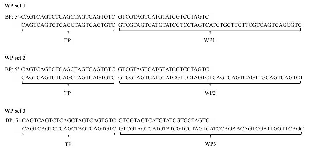
Figure 1. Three walker primer (WP) sets used in this study and the interrelationship of WP, bridging primer (BP), and tail primer (TP) in a WP set.
Critical: WP (50 nt), BP (50 nt), and TP (25 nt) are random oligo DNAs, with Tm values of 70–75, 70–75, and 60–65 °C, respectively. BP is made by attaching TP to the 5′ end of WP 5′ region.
Note: Design three WP sets so as to perform three parallel sets of bridging PCRs in a WP. The three WPs have an identical 5′ region (25 nt) but completely different 3′ regions (25 nt). The identical 5′ region means that only one BP and one TP are required, while the different 3′ regions endow WPs with individualized annealing patterns. Therefore, the three WP sets are actually constituted by five primers, namely, three WPs, one BP, and one TP.
1. Design of WP.
a. Open the Oligo 7 software, click File and New Sequence to show Edit Sequence dialog box; type in a 50 nt arbitrary sequence in Edit Sequence dialog box (Figure 2A) and then sequentially click Accept/Discard and Accept to accept the input sequence (Figure 2B).
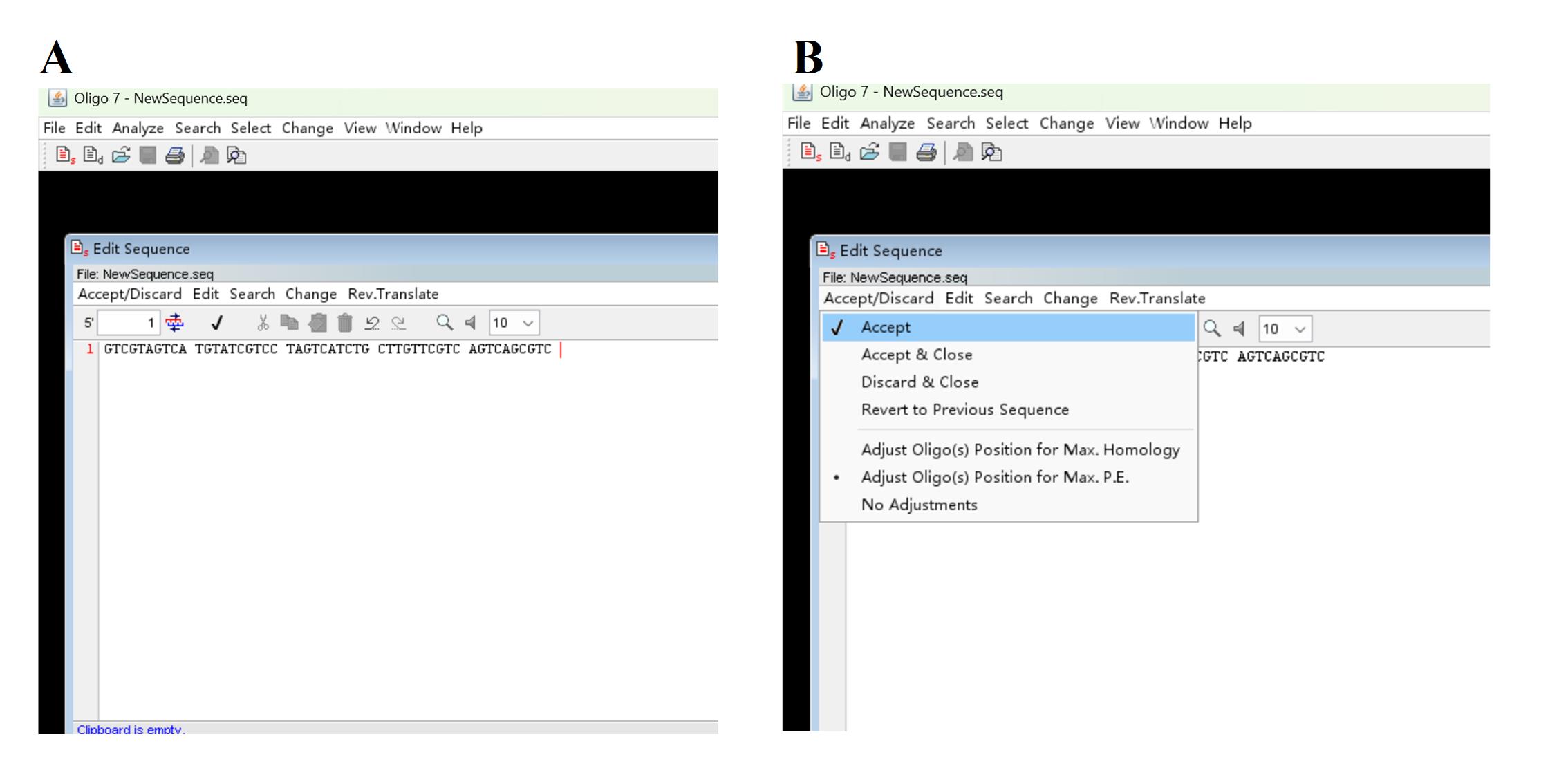
Figure 2. Screenshots showing how to input an arbitrary primer sequence. (A) Discovery of Edit Sequence dialog box. (B) How to accept the input sequence.
b. Click Analyze, Duplex Formation, and Current Oligo (Figure 3A) to assess primer dimer(s) (Figure 3B).
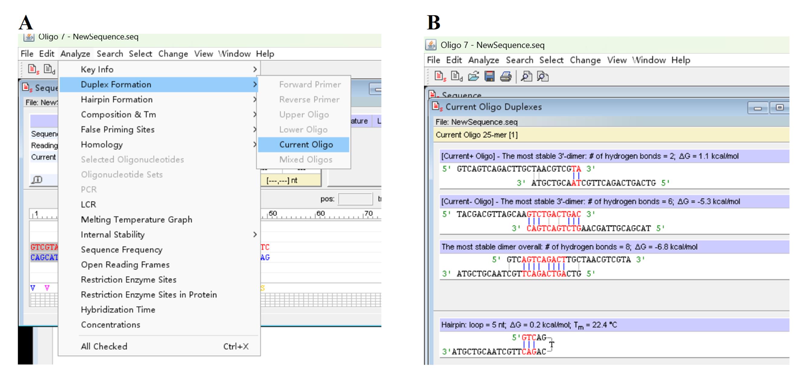
Figure 3. Screenshots showing how to assess primer dimer(s). (A) Discovery of Duplex Formation and Current Oligo under Analyze tab. (B) Output dimer(s).
c. Click Analyze, Hairpin Formation, and Current Oligo (Figure 4A) to assess primer hairpin(s) (Figure 4B).
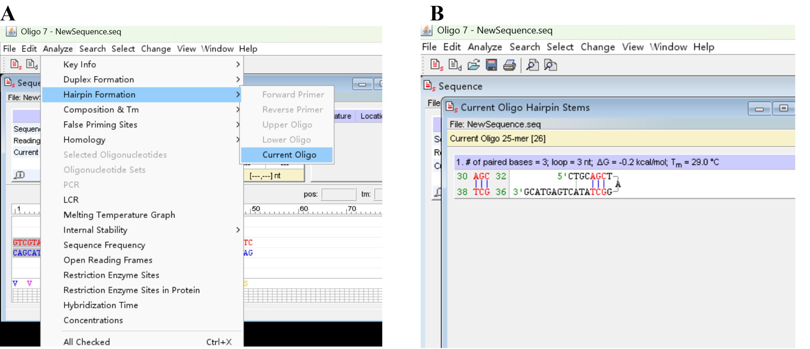
Figure 4. Screenshots showing how to check primer hairpin(s). (A) Discovery of Hairpin Formation and Current Oligo under Analyze tab. (B) Output hairpin(s).
Note: Edit this primer and then re-assess it if it shows a severe dimer(s) or hairpin(s) with Tm ≥ 40 °C.
d. Return to the Edit Sequence dialog box (Figure 2A) by clicking Edit and Entire Sequence (Figure 5A). Change the sequence according to the above analysis outcomes; click Accept/Discard and Accept (Figure 2B) and then minimize this dialog box to show the dialog box shown in Figure 3A.
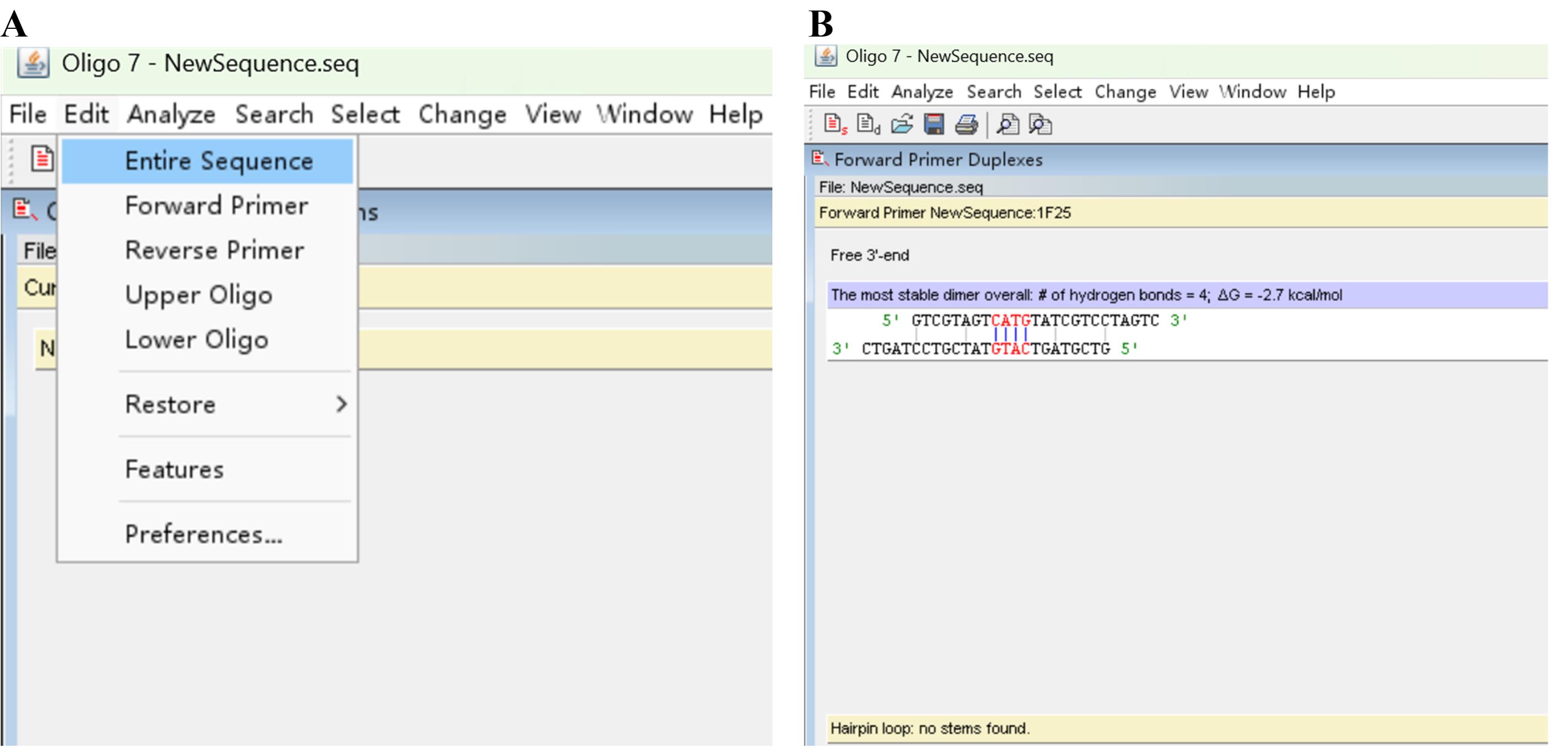
Figure 5. Screenshots showing how to optimize the primer. (A) Discovery of Edit Sequence dialog box. (B) Output primer hairpin(s).
e. Repeat steps A1b–c to evaluate the sequence until satisfactory WP (Figure 5B) is obtained.
Notes:
1. The WP shown in Figure 5B is acceptable because it has no obvious primer dimer or hairpin.
2. Fix the 5′ region (25 nt) of this WP, then add another arbitrary sequence (25 nt) to its 3′ end; repeat steps A1b–c to evaluate this new primer until it is satisfactory. Three WPs are designed in this study.
2. Design a satisfactory TP by repeating steps A1a–e, just like designing the WP.
3. Create a BP by attaching the TP to the 5′ end of WP 5′ region (25 nt).
Note: Assess this BP by repeating steps A1b–c until a satisfactory BP is created.
4. Pick SSP.
a. Open the Oligo 7 software and click File and Open to input the known DNA sequence.
b. Click Change and Current Oligo Length to select and define the length of SSP (Figure 6A).
c. Assess the SSP by repeating steps A1b–c (Figure 6B).
Note: Redesign the SSP and evaluate it by repeating steps A1b–c until a satisfactory one (Figure 6B) is obtained, if the current SSP forms a severe primer dimer(s) or hairpin(s) with Tm ≥ 40 °C.
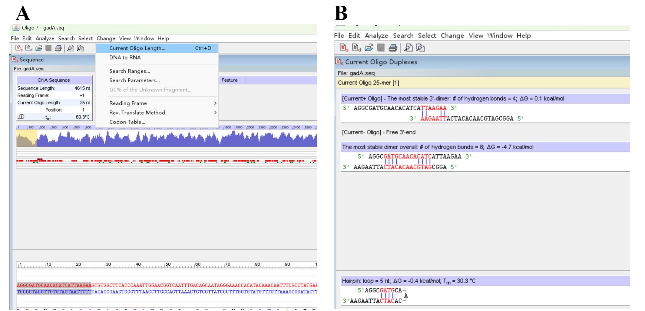
Figure 6. Screenshots showing how to pick a sequence-specific primer (SSP). (A) Discovery of Current Oligo Length. (B) Output primer dimer(s) and hairpin(s).
Critical: The SSP should have a Tm of 60–65 °C according to Mazars et al. [34].
B. Bridging PCR procedure
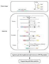
A bridging PCR set contains three rounds of nested PCR. The primary PCR is driven by WP and SSP1, the secondary PCR is driven by TP, BP, and SSP2, and the tertiary PCR is driven by TP and SSP3 (Figure 7).
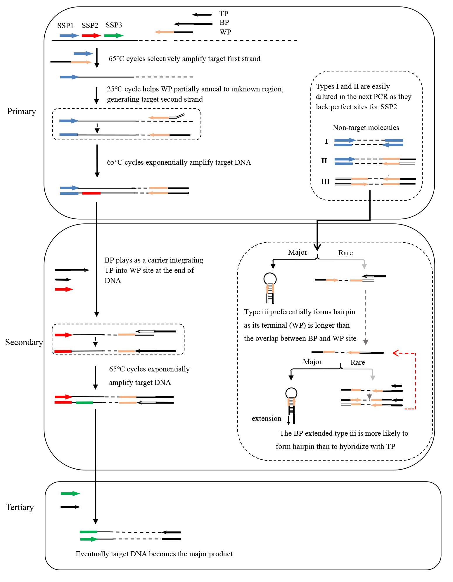
Figure 7. Schematic diagram of bridging PCR. WP: walker primer; BP: bridging primer; TP: tail primer; SSP: sequence-specific primer. Thin solid lines: known sequences; thin dotted lines: unknown sequences.
Critical: The working concentration of BP is only one twenty-fifth of TP or SSP2.
1. Primary bridging PCR.
a. Pipette primary bridging PCR components (Table 1) into a PCR tube.
Table 1. Primary bridging PCR mix
| Reagent | Final concentration | Volume (μL) |
|---|---|---|
| Genomic DNA | Microbe, 10–100 ng/μL; or rice, 100–1,000 ng/μL | 1 |
| LA Taq polymerase (5 U/μL) | 0.05 U/μL | 0.5 |
| WP (10 μM) | 0.2 μM | 1 |
| SSP1 (10 μM) | 0.2 μM | 1 |
| 10× LA PCR buffer II (Mg2+ plus) | 1× | 5 |
| dNTP mixture (2.5 mM each) | 0.4 mM each | 8 |
| Ultrapure water | n/a | 33.5 |
| Total | n/a | 50 |
b. Mix the components well.
c. Centrifuge the tube at 3,000× g for 20 s at 4 °C.
d. Run PCR amplification (Table 2).
Table 2. Primary bridging PCR cycling conditions
| Step | Temperature | Duration | Cycle |
| Initial denaturation | 95 °C | 1 min | 1 |
| Denaturation | 95 °C | 20 s | 5 |
| Annealing | 65 °C | 30 s | |
| Extension | 72 °C | 2 min | |
| Denaturation | 95 °C | 20 s | 1 |
| Annealing | 25 °C | 30 s | |
| Extension | 72 °C | 2 min | |
| Denaturation | 95 °C | 20 s | 30 |
| Annealing | 65 °C | 30 s | |
| Extension | 72 °C | 3 min | |
| Final extension | 72 °C | 5 min | 1 |
| Hold | 4 | forever | 1 |
e. Take 1 μL of the product as template for secondary bridging PCR.
f. Store the remaining product at -20 °C.
2. Secondary bridging PCR.
a. Pipette secondary bridging PCR components (Table 3) into a PCR tube.
Table 3. Secondary bridging PCR mix
| Reagent | Final concentration | Volume (μL) |
|---|---|---|
| Primary product | n/a | 1 |
| LA Taq polymerase (5 U/μL) | 0.05 U/μL | 0.5 |
| TP (10 μM) | 0.2 μM | 1 |
| SSP2 (10 μM) | 0.2 μM | 1 |
| BP (1uM) | 8 nM | 0.4 |
| 10× LA PCR buffer II (Mg2+ plus) | 1× | 5 |
| dNTP mixture (2.5 mM each) | 0.4 mM each | 8 |
| Ultrapure water | n/a | 33.1 |
| Total | n/a | 50 |
Critical: The working concentration of BP is only one twenty-fifth of TP or SSP2.
Note: If necessary, dilute the primary bridging PCR product 10–1,000 times.
b. Mix the components well.
c. Centrifuge the tube at 3,000× g for 20 s at 4 °C.
d. Run PCR amplification (Table 4).
Table 4. Secondary bridging PCR cycling conditions
| Step | Temperature | Duration | Cycle |
| Initial denaturation | 95 °C | 1 min | 25–45 |
| Denaturation | 95 °C | 20 S | |
| Annealing | 65 °C | 30 S | |
| Extension | 72 °C | 1.5 min | |
| Final extension | 72 °C | 5 min |
e. Put the PCR product onto ice.
f. Take 1 μL of the product as the template for tertiary bridging PCR.
g. Store the remaining product at -20 °C.
3. Tertiary bridging PCR.
a. Pipette tertiary bridging PCR components (Table 5) into a PCR tube.
Table 5. Tertiary bridging PCR mix
| Reagent | Final concentration | Volume (μL) |
|---|---|---|
| Secondary PCR product | n/a | 1 |
| LA Taq polymerase (5 U/μL) | 0.05 U/μL | 0.5 |
| TP (10 μM) | 0.2 μM | 1 |
| SSP3 (10 μM) | 0.2 μM | 1 |
| 10× LA PCR buffer II (Mg2+ plus) | 1× | 5 |
| dNTP mixture (2.5 mM each) | 0.4 mM each | 8 |
| Ultrapure water | n/a | 33.5 |
| Total | n/a | 50 |
Critical: Dilute the secondary bridging PCR product 10–1,000 times if necessary.
b. Mix the components well.
c. Centrifuge at 3,000× g for 20 s at 4 °C.
d. Run PCR amplification (Table 6).
Table 6. Tertiary fork PCR cycling conditions
| Step | Temperature | Duration | Cycle |
| Initial denaturation | 95 °C | 1 min | 15–30 |
| Denaturation | 95 °C | 20 S | |
| Annealing | 65 °C | 30 S | |
| Extension | 72 °C | 1.5 min | |
| Final extension | 72 °C | 5 min | |
| Hold | 4 | forever |
e. Store the PCR product at -20 °C.
C. Electrophoresis
1. Add 5 μL of each bridging PCR product and 1 μL of 6× loading buffer.
2. Transfer the mixture into a 1.5% agarose gel supplemented with 1× Goldview nucleic acid gel stain.
3. Electrophorese at a voltage of 5 V/cm for 30 min.
4. Check the gel using the ChemiDoc XRS+ imaging system (Figure 8).
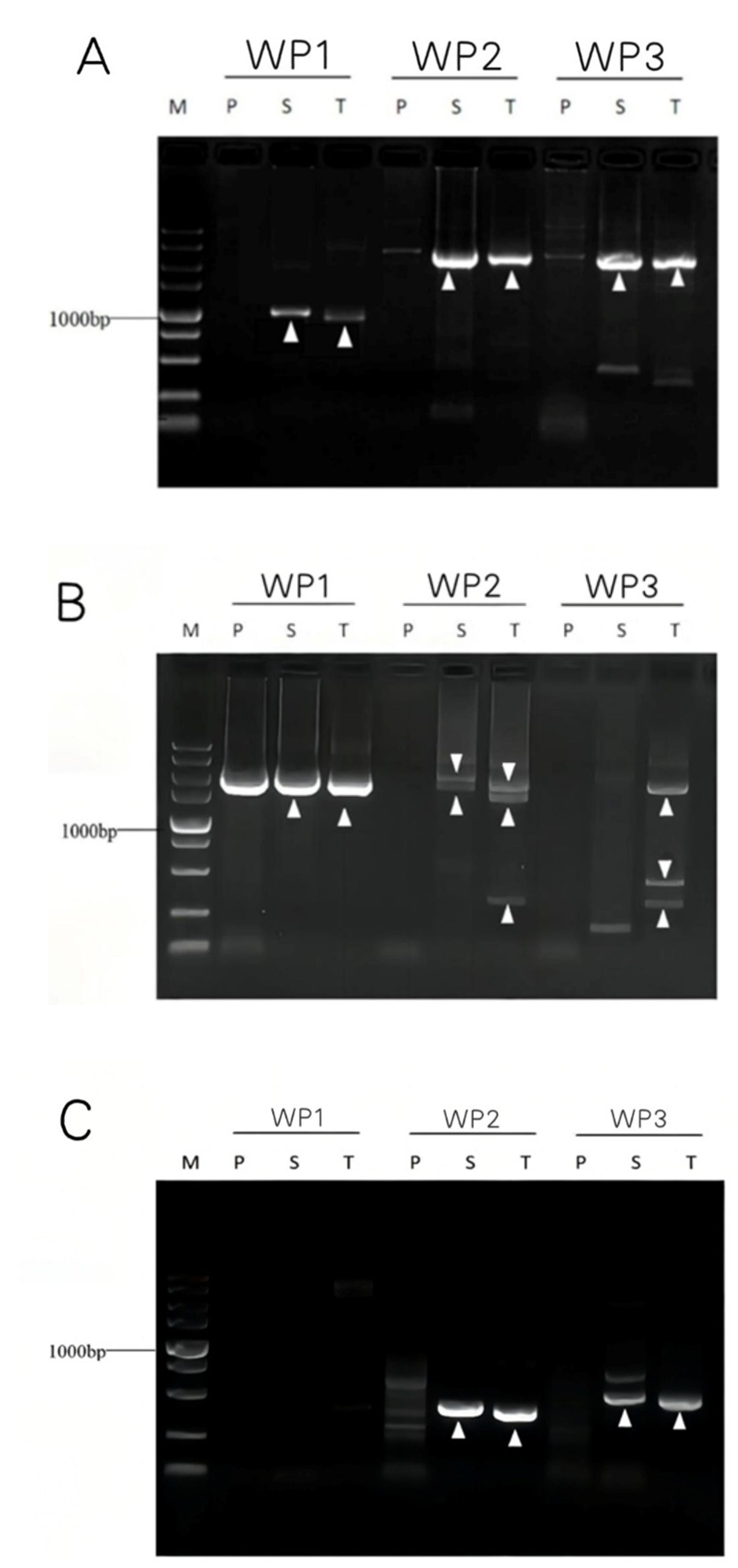
Figure 8. Genome walking of gadA (A) and gadR (B) of Levilactobacillus brevis CD 0817 and hyg (C) of rice. WP1, WP2, and WP3 denote the three parallel bridging PCR sets. P: primary PCR; S: secondary PCR; T: Tertiary PCR; and M: DNA5000 Marker. The white arrowheads indicate the target DNA bands.
D. Recovery of PCR product
1. Mix 40 μL of secondary/tertiary bridging PCR product and 8 μL of 6× loading buffer.
2. Transfer the mixture into a 1.5% agarose gel supplemented with 1× Goldview nucleic acid gel stain.
3. Electrophorese at a voltage of 5 V/cm for 30 min.
4. Check the gel using the ChemiDoc XRS+ imaging system (Figure 9) and cut out the target DNA band(s) with a knife.
5. Purify the DNA band(s) from the cut gel using the Mini-BEST Agarose Gel DNA Extraction kit v4.0.
E. DNA sequencing
Mail the purified product(s) to Sangon Biotech Co., Ltd for sequencing.
Data analysis
1. Analyze the sequencing data using the MegAlign software.
a. Open the software, then click File and Enter Sequences to input DNA sequences to be analyzed (Figure 9).
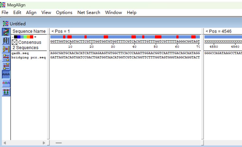
Figure 9. Screenshots showing how to input DNA sequences
b. Click Align and By Clustal W Method (Figure 10A) to get the result (Figure 10B).
Note: The experiment is considered successful if the SSP3-sided segment of the bridging PCR product overlaps the known DNA (Figure 10B).
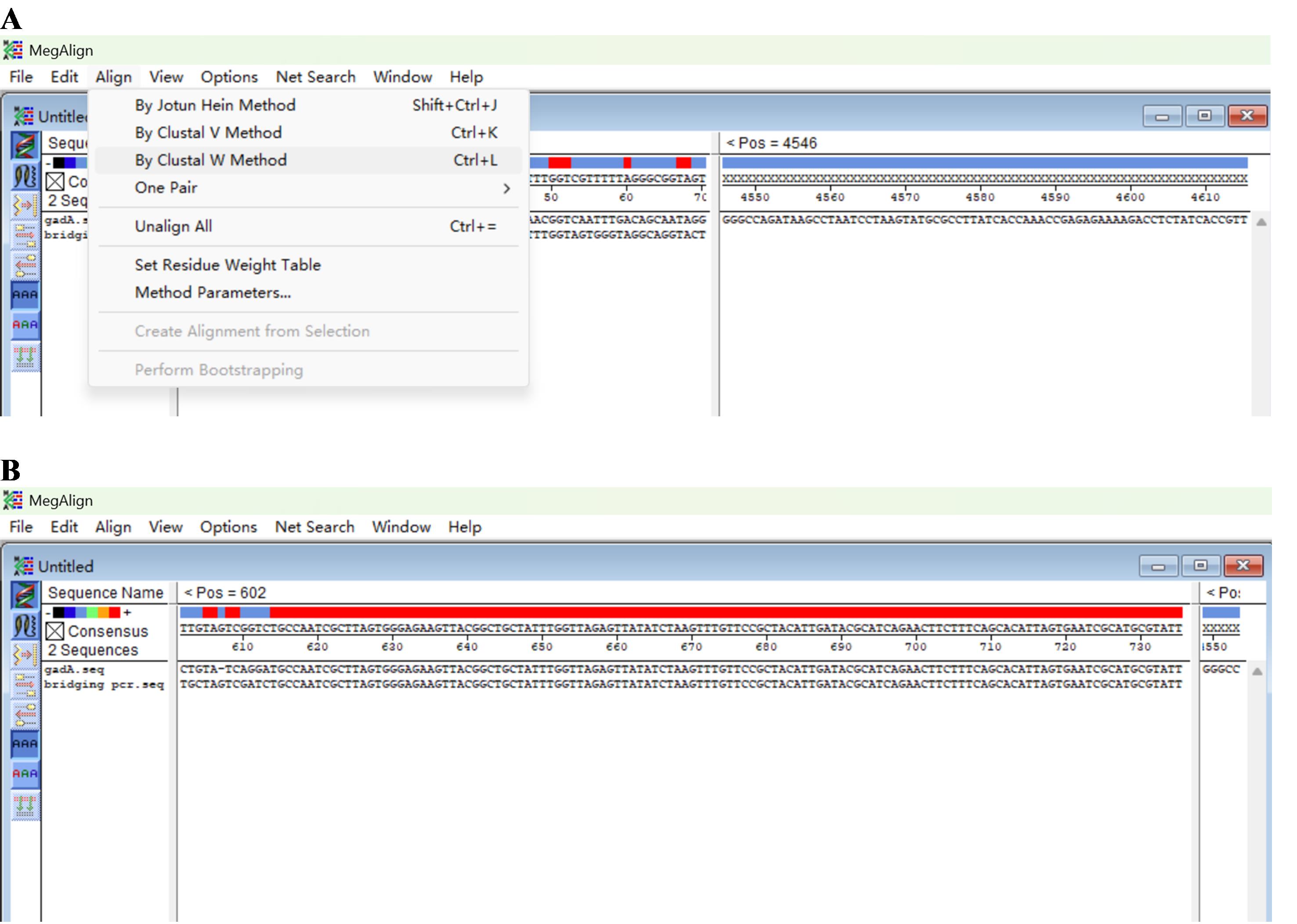
Figure 10. Screenshots showing how to analyze the input sequences. (A) Discovery of By Clustal W Method. (B) Final outcome.
Validation of protocol
This protocol or parts of it has been used and validated in the following research articles:
Lin et al. [1]. Bridging PCR: An Efficient and Reliable Scheme Implemented for genome walking. Current Issues in Molecular Biology (Figure 8).
General notes and troubleshooting
General notes
1. The bridging PCR protocol is a universal genome-walking tool.
2. Secondary bridging PCR amplification can generally release a positive result.
3. Simultaneously performing parallel bridging PCRs will improve the success and efficiency of genome walking.
4. In secondary bridging PCR, the working concentration of BP is very low, and its role is just to introduce a TP sequence to the 5′ end of the WP 5′ region. The real amplifiers are TP and SSP3.
5. The ends of non-target DNA primed by WP are lengthened by BP. This DNA cannot be amplified by TP in the next PCR, because it forms a hairpin structure via the lengthened ends.
Troubleshooting
Problem 1: Secondary/tertiary bridging PCR does not produce target DNA(s).
Possible causes: Non-target amplification efficiency is high, or target amplification is insufficient.
Solutions: Dilute the previous product properly and use it as the template for the next PCR. If this is still ineffective, redesign an SSP set.
Problem 2: DNA band(s) cannot be directly sequenced.
Possible cause: There may be interference from non-target background.
Solution: T-clone the target DNA band and then sequence [35].
Problem 3: The DNA band(s) are not the target.
Possible cause: There may be sites homologous to SSP(s) in other regions of the genome.
Solution: Redesign an SSP set.
Acknowledgments
This study was supported by the State Key Laboratory of Food Science and Resources (SKLF-ZZB-202523), Nanchang University, China, and the Jiangxi Provincial Department of Science and Technology (20225BCJ22023), China. This protocol has been originally described and validated in Current Issues in Molecular Biology [1].
Competing interests
The authors declare no competing interests.
References
- Lin, Z., Wei, C., Pei, J. and Li, H. (2023). Bridging PCR: An Efficient and Reliable Scheme Implemented for Genome-Walking. Curr Issues Mol Biol. 45(1): 501–511. https://doi.org/10.3390/cimb45010033
- Gao, D., Pan, Z., Pan, H., Gu, Y. and Li, H. (2025). Center Degenerated Walking-Primer PCR: A Novel and Universal Genome-Walking Method. Curr Issues Mol Biol. 47(8): 602. https://doi.org/10.3390/cimb47080602
- Acevedo, J. P., Reyes, F., Parra, L. P., Salazar, O., Andrews, B. A. and Asenjo, J. A. (2008). Cloning of complete genes for novel hydrolytic enzymes from Antarctic sea water bacteria by use of an improved genome walking technique. J Biotechnol. 133(3): 277–286. https://doi.org/10.1016/j.jbiotec.2007.10.004
- Siebert, P. D., Chenchik, A., Kellogg, D. E., Lukyanov, K. A. and Lukyanov, S. A. (1995). An improved PCR method for walking in uncloned genomic DNA. Nucleic Acids Res. 23(6): 1087–1088. https://doi.org/10.1093/nar/23.6.1087
- Wang, R., Gu, Y., Chen, H., Tian, B. and Li, H. (2025). Uracil base PCR implemented for reliable DNA walking. Anal Biochem. 696: 115697. https://doi.org/10.1016/j.ab.2024.115697
- Liu, Y. G. and Whittier, R. F. (1995). Thermal asymmetric interlaced PCR: automatable amplification and sequencing of insert end fragments from P1 and YAC clones for chromosome walking. Genomics. 25(3): 674–681. https://doi.org/10.1016/0888-7543(95)80010-j
- Chen, H., Tian, B., Wang, R., Pan, Z., Gao, D. and Li, H. (2025). Uracil walking primer PCR: An accurate and efficient genome-walking tool. J Genet Eng Biotechnol. 23(2): 100478. https://doi.org/10.1016/j.jgeb.2025.100478
- Yu, Z., Wang, D., Lin, Z. and Li, H. (2025). Protocol to Mine Unknown Flanking DNA Using PER-PCR for Genome Walking. Bio Protoc. 15(4): e5188. https://doi.org/10.21769/bioprotoc.5188
- Tian, B., Wu, H., Wang, R., Chen, H. and Li, H. (2024). N7-Ended Walker PCR: An Efficient Genome-Walking Tool. Biochem Genet. 63(4): 3758–3772. https://doi.org/10.1007/s10528-024-10896-1
- Pei, J., Sun, T., Wang, L., Pan, Z., Guo, X. and Li, H. (2022). Fusion primer driven racket PCR: A novel tool for genome walking. Front Genet. 13: e969840. https://doi.org/10.3389/fgene.2022.969840
- Li, H., Wei, C., Pan, Z. and Liu, X. (2024). Arbitrarily suffixed sequence-specific primer PCR for reliable genome walking: Taking genome walkings of Levilactobacillus brevis and rice as examples. Iran J Biotechnol. 22(4): 106–111. https://doi.org/10.30498/ijb.2024.449960.3896
- Okulova, E. S., Burlakovskiy, M. S. and Lutova, L. A. (2024). PCR-based genome walking methods (review). Ecol Genet. 22(1): 75–104. https://doi.org/10.17816/ecogen624820
- Chang, K., Wang, Q., Shi, X., Wang, S., Wu, H., Nie, L. and Li, H. (2018). Stepwise partially overlapping primer-based PCR for genome walking. AMB Express. 8(1): 77. https://doi.org/10.1186/s13568-018-0610-7
- Wu, H., Pan, H. and Li, H. (2025). Protocol to Retrieve Unknown Flanking DNA Using Fork PCR for Genome Walking. Bio Protoc. 15(2): e5161. https://doi.org/10.21769/bioprotoc.5161
- Wei, C., Lin, Z., Pei, J., Pan, H. and Li, H. (2023). Semi-Site-Specific Primer PCR: A Simple but Reliable Genome-Walking Tool. Curr Issues Mol Biol. 45(1): 512–523. https://doi.org/10.3390/cimb45010034
- Wang, L., Jia, M., Li, Z., Liu, X., Sun, T., Pei, J., Wei, C., Lin, Z. and Li, H. (2022). Wristwatch PCR: A Versatile and Efficient Genome Walking Strategy. Front Bioeng Biotechnol. 10: e792848. https://doi.org/10.3389/fbioe.2022.792848
- Sun, T., Jia, M., Wang, L., Li, Z., Lin, Z., Wei, C., Pei, J. and Li, H. (2022). DAR-PCR: a new tool for efficient retrieval of unknown flanking genomic DNA. AMB Express. 12(1): 131. https://doi.org/10.1186/s13568-022-01471-1
- Kotik, M. (2009). Novel genes retrieved from environmental DNA by polymerase chain reaction: Current genome-walking techniques for future metagenome applications. J Biotechnol. 144(2): 75–82. https://doi.org/10.1016/j.jbiotec.2009.08.013
- Wang, L., Jia, M., Li, Z., Liu, X., Sun, T., Pei, J., Wei, C., Lin, Z. and Li, H. (2023). Protocol to access unknown flanking DNA sequences using Wristwatch-PCR for genome-walking. STAR Protoc. 4(1): 102037. https://doi.org/10.1016/j.xpro.2022.102037
- Evangelene Christy, S. M. and Arun, V. (2024). Isolation of actin regulatory region from medicinal plants by thermal asymmetric interlaced PCR (TAIL PCR) and its bioinformatic analysis. Braz J Bot. 47(1): 67–78. https://doi.org/10.1007/s40415-023-00971-z
- Wang, Z., Ye, S., Li, J., Zheng, B., Bao, M. and Ning, G. (2011). Fusion primer and nested integrated PCR (FPNI-PCR): a new high-efficiency strategy for rapid chromosome walking or flanking sequence cloning. BMC Biotech. 11(1): 109. https://doi.org/10.1186/1472-6750-11-109
- Li, H., Ding, D., Cao, Y., Yu, B., Guo, L. and Liu, X. (2015). Partially Overlapping Primer-Based PCR for Genome Walking. PLoS One. 10(3): e0120139. https://doi.org/10.1371/journal.pone.0120139
- Jia, M., Ding, D., Liu, X. and Li, H. (2025). Protocol to Identify Unknown Flanking DNA Using Partially Overlapping Primer-based PCR for Genome Walking. Bio Protoc. 15(3): e5172. https://doi.org/10.21769/bioprotoc.5172
- Pan, H., Guo, X., Pan, Z., Wang, R., Tian, B. and Li, H. (2023). Fork PCR: a universal and efficient genome-walking tool. Front Microbiol. 14: e1265580. https://doi.org/10.3389/fmicb.2023.1265580
- Chen, H., Wei, C., Lin, Z., Pei, J., Pan, H. and Li, H. (2024). Protocol to retrieve unknown flanking DNA sequences using semi-site-specific PCR-based genome walking. STAR Protoc. 5(1): 102864. https://doi.org/10.1016/j.xpro.2024.102864
- Li, H., Lin, Z., Guo, X., Pan, Z., Pan, H. and Wang, D. (2024). Primer extension refractory PCR: an efficient and reliable genome walking method. Mol Genet Genomics. 299(1): 27. https://doi.org/10.1007/s00438-024-02126-5
- Guo, X., Zhu, Y., Pan, Z., Pan, H. and Li, H. (2024). Single primer site-specific nested PCR for accurate and rapid genome-walking. J Microbiol Methods. 220: 106926. https://doi.org/10.1016/j.mimet.2024.106926
- Wang, L., Jia, M., Gao, D. and Li, H. (2024). Hybrid substrate-based pH autobuffering GABA fermentation by Levilactobacillus brevis CD0817. Bioprocess Biosyst Eng. 47(12): 2101–2110. https://doi.org/10.1007/s00449-024-03088-z
- Li, H., Pei, J., Wei, C., Lin, Z., Pan, H., Pan, Z., Guo, X. and Yu, Z. (2023). Sodium-Ion-Free Fermentative Production of GABA with Levilactobacillus brevis CD0817. Metabolites. 13(5): 608. https://doi.org/10.3390/metabo13050608
- Li, H., Sun, T., Jia, M., Wang, L., Wei, C., Pei, J., Lin, Z. and Wang, S. (2022). Production of Gamma-Aminobutyric Acid by Levilactobacillus brevis CD0817 by Coupling Fermentation with Self-Buffered Whole-Cell Catalysis. Fermentation. 8(7): 321. https://doi.org/10.3390/fermentation8070321
- Jia, M., Zhu, Y., Wang, L., Sun, T., Pan, H. and Li, H. (2022). pH Auto-Sustain-Based Fermentation Supports Efficient Gamma-Aminobutyric Acid Production by Lactobacillus brevis CD0817. Fermentation. 8(5): 208. https://doi.org/10.3390/fermentation8050208
- Gao, D., Chang, K., Ding, G., Wu, H., Chen, Y., Jia, M., Liu, X., Wang, S., Jin, Y., Pan, H., et al. (2019). Genomic insights into a robust gamma-aminobutyric acid-producer Lactobacillus brevis CD0817. AMB Express. 9(1): 72. https://doi.org/10.1186/s13568-019-0799-0
- Li, H., Wang, L., Nie, L., Liu, X. and Fu, J. (2023). Sensitivity Intensified Ninhydrin-Based Chromogenic System by Ethanol-Ethyl Acetate: Application to Relative Quantitation of GABA. Metabolites. 13(2): 283. https://doi.org/10.3390/metabo13020283
- Mazars, G. R., Moyret, C., Jeanteur, P. and Theillet, C. G. (1991). Direct sequencing by thermal asymmetric PCR. Nucleic Acids Res. 19(17): 4783–4783. https://doi.org/10.1093/nar/19.17.4783
- Zhou, M. Y., Clark, S. E. and Gomezsanchez, C. E. (1995). Universal cloning method by TA strategy. Biotechniques. 19(1): 34–35. https://pubmed.ncbi.nlm.nih.gov/7669292/
Article Information
Publication history
Received: Sep 22, 2025
Accepted: Nov 2, 2025
Available online: Nov 11, 2025
Published: Dec 5, 2025
Copyright
© 2025 The Author(s); This is an open access article under the CC BY-NC license (https://creativecommons.org/licenses/by-nc/4.0/).
How to cite
Li, M., Gu, Y., Tang, Q. and Li, H. (2025). Bridging PCR-Based Genome-Walking Protocol. Bio-protocol 15(23): e5531. DOI: 10.21769/BioProtoc.5531.
Category
Molecular Biology > DNA > Genome walking
Molecular Biology > DNA > PCR
Molecular Biology > DNA > DNA cloning
Do you have any questions about this protocol?
Post your question to gather feedback from the community. We will also invite the authors of this article to respond.