- Protocols

- Articles and Issues
- For Authors
- About
- Become a Reviewer

A Step-by-Step Computational Protocol for Functional Annotation and Structural Modelling of Insect Chemosensory Proteins

Published: Vol 15, Iss 22, Nov 20, 2025 DOI: 10.21769/BioProtoc.5523 Views: 1667
Reviewed by: Madhumala K. SadanandappaAnonymous reviewer(s)

Protocol Collections
Comprehensive collections of detailed, peer-reviewed protocols focusing on specific topics


Related protocols
Abstract
Insects rely on chemosensory proteins, including gustatory receptors, to detect chemical cues that regulate feeding, mating, and oviposition behaviours. Conventional approaches for studying these proteins are limited by the scarcity of experimentally resolved structures, especially in non-model pest species. Here, we present a reproducible computational protocol for the identification, functional annotation, and structural modelling of insect chemosensory proteins, demonstrated using gustatory receptors from the red palm weevil (Rhynchophorus ferrugineus) as an example. The protocol integrates publicly available sequence data with OmicsBox for functional annotation and ColabFold for high-confidence structure prediction, providing a step-by-step framework that can be applied to genome-derived or transcriptomic datasets. The workflow is designed for broad applicability across insect species and generates structurally reliable protein models suitable for downstream applications such as ligand docking or molecular dynamics simulations. By bridging functional annotation with structural characterisation, this protocol enables reproducible studies of chemosensory proteins in agricultural and ecological contexts and supports the development of novel pest management strategies.
Key features
• Designed for insect chemosensory research, demonstrated using gustatory receptors from the red palm weevil (Rhynchophorus ferrugineus) as a representative pest species.
• Combines OmicsBox for functional annotation with ColabFold for reproducible, high-confidence protein structure prediction in a streamlined workflow.
• Accepts input from genome assemblies, transcriptomic datasets, or curated sequence databases, enabling broad application across model and non-model insects.
• Produces reliable structural models suitable for downstream studies, including ligand screening, molecular dynamics simulations, and comparative evolutionary analyses.
Keywords: Gustatory receptorsGraphical overview
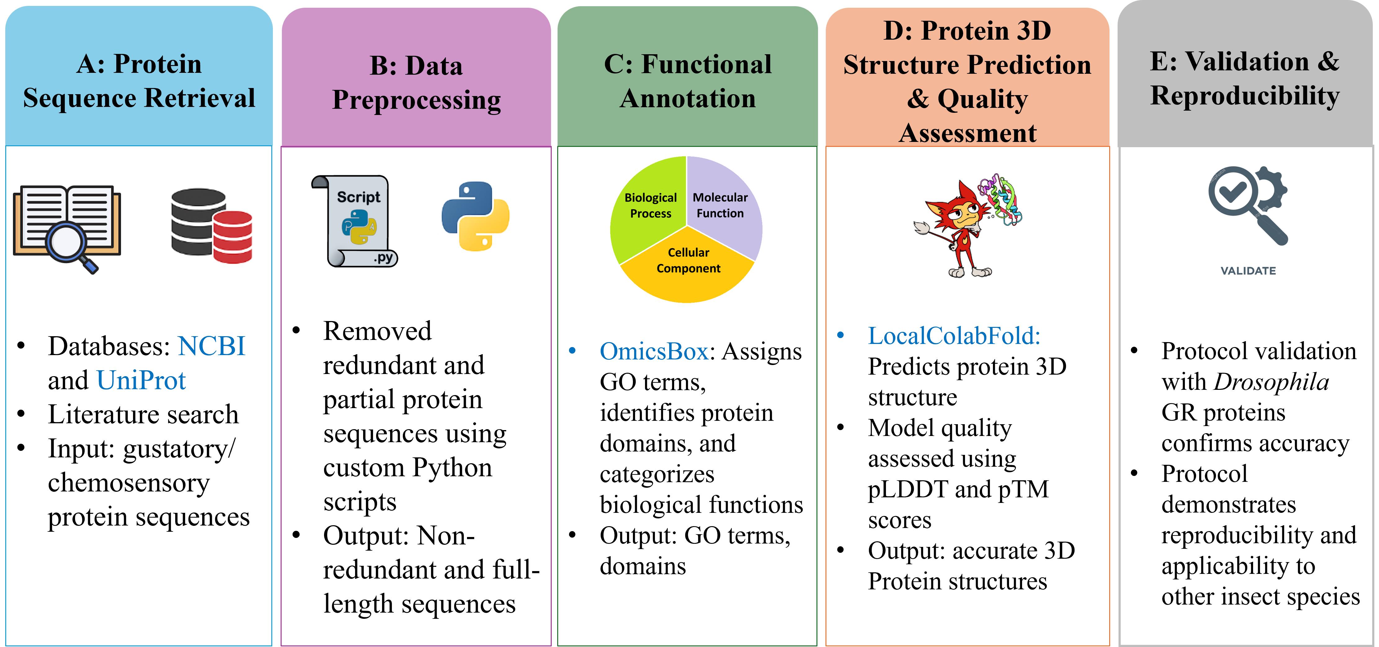
Computational workflow for identification, annotation, and structural characterisation of insect gustatory proteins. Databases and software are shown in blue.
Background
Rhynchophorus ferrugineus, commonly known as the red palm weevil (RPW), is a highly invasive pest that poses a serious threat to palm species globally, particularly date, coconut, and oil palms. Native to the Middle East, RPW has rapidly expanded across tropical and subtropical regions, causing substantial agricultural and economic damage [1,2]. Its concealed infestation behaviour and the difficulty of early detection contribute to its ecological impact [3]. Despite extensive management efforts, control remains challenging due to its complex life cycle, adaptability, and increasing resistance to conventional methods. Current strategies, including chemical insecticides and pheromone traps [4], have shown limited success, hindered by the development of resistance and inefficient monitoring systems [5]. These limitations underscore the need for molecular-level approaches to disrupt pest behaviour. Targeting insect chemosensory systems offers a promising alternative, as these systems are essential for survival and reproduction. Chemosensory proteins, particularly gustatory receptors (GRs), which mediate responses to non-volatile compounds involved in feeding and mating, are particularly relevant. However, GRs in RPW remain poorly characterised, and no experimentally resolved structures are currently available [6,7], which complicates molecular intervention efforts.
To address this gap, we present an integrated computational pipeline that combines OmicsBox-based sequence annotation with high-accuracy structural prediction. Functional annotation performed with OmicsBox [8] enables the reliable identification of candidate GRs, while structure prediction with LocalColabFold [9] generates three-dimensional models enriched with confidence metrics such as pLDDT (predicted local distance difference test) and pTM (predicted template modelling) scores and PAE (predicted alignment error). This dual-layered approach provides not only accurate identification of GRs but also structural insights, including the prediction of potential ligand-binding sites. Such integrative information is critical for advancing molecular studies of insect chemosensation and supports downstream applications such as protein-ligand docking and virtual screening. Previous bioinformatics efforts have generally applied these tools independently, depending on the scope of analysis. OmicsBox has been extensively used for transcriptome and genome annotation in insects, such as the cabbage webworm (Hellula undalis) [10] and the boll weevil (Anthonomus grandis grandis) [11], but these studies were limited to sequence-level analyses. Conversely, ColabFold has gained attention for protein modelling [12], though its applications often depend on pre-annotated datasets without integrated annotation workflows. By combining both strategies into a single reproducible pipeline, our protocol overcomes these limitations and enables a more comprehensive characterisation of GR proteins, particularly in non-model pest species.
This workflow was validated through comparison of RPW GRs with proteins from the well-characterised fruit fly (Drosophila melanogaster), confirming its accuracy and reproducibility. This benchmarking demonstrates the pipeline’s ability to generate consistent, biologically meaningful results and highlights its applicability across insect species. Unlike previous studies that addressed annotation or structural modelling separately, our protocol integrates both, providing a holistic characterisation of GR proteins. Its reproducibility, adaptability, and biological relevance make it a reusable framework for advancing insect chemosensory research and supporting innovative pest management strategies.
Software and datasets
1. Data (NCBI, May 2025, public domain, https://www.ncbi.nlm.nih.gov/protein/, free)
2. Data (UniProt, May 2025, CC BY 4.0, https://www.uniprot.org/, free)
3. Script/Code (Custom Python Scripts, May 2025, user-defined, https://github.com/norazlannm/Protein-structure-annotation-and-3D-model-generation/, free)
4. Module [Biopython (Python module), V1.85 (via pip), May 2025, Biopython License, https://biopython.org/wiki/Download, free]
5. Software 1 (OmicsBox, V3.4, June 2025, commercial, https://www.biobam.com/download-omicsbox/, 7-day free trial; paid subscription required thereafter)
6. Software 2 (LocalColabFold, V1.5.5, June 2025, MIT License, https://github.com/YoshitakaMo/localcolabfold, free)
7. Workflow manager
a. Desktop/laptop system
b. AMD Ryzen 7700x, 8-core CPU
c. 64 GB DDR5 RAM, 2 TB SSD
d. NVIDIA RTX 4070 Ti GPU
Software configuration
LocalColabFold was installed using the standard installation instructions from the official GitHub page (https://github.com/YoshitakaMo/localcolabfold), without any special configuration files.
Software dependencies
• LocalColabFold: Requires Python version 3.8 or higher, CUDA version 11.1 or higher, and GCC version 9.0 or higher.
• Custom Python scripts: Depend on the Biopython library.
• Biopython: Requires Python 3.7 or higher.
System requirements
The following hardware requirements are suggested for computational implementation to improve reproducibility:
1. Processor: Multi-core CPU; minimum: ≥4 cores, base clock speed ≥2.5 GHz; recommended: ≥8 cores, base clock speed ≥3.0 GHz.
2. Memory: 8 GB (minimum), 16 GB RAM (recommended).
Note: 16 GB RAM is sufficient for OmicsBox analysis and small protein size, and more than 16 GB RAM is required for large-scale protein modelling using LocalColabFold to avoid memory limitations.
3. Storage: ≥200 GB available disk space for databases (e.g., AlphaFold database ~100 GB), intermediate files (~50 GB, may vary depending on project size), and output files (~50 GB, depends on number and size of the models).
4. Graphics: NVIDIA GPU with CUDA support (≥8 GB VRAM) is recommended for efficient LocalColabFold execution (e.g., RTX 3060 or higher), but LocalColabFold can also run without a GPU, albeit more slowly. For single-protein modelling, ColabFold v1.5.5 notebook mode can be used without a dedicated GPU (https://colab.research.google.com/github/sokrypton/ColabFold/blob/main/AlphaFold2.ipynb).
Note: While these specifications are sufficient for most analyses, a higher-performance workstation (≥8 cores, ≥64 GB RAM, ≥2 TB SSD storage, and GPU) is strongly recommended for large datasets and multiple protein modelling tasks to reduce runtime and improve computational efficiency significantly.
Software/OS requirements
• Operating system: Linux (Ubuntu 20.04+ recommended), Windows 10/11 (for LocalColabFold on WSL2), or macOS version 10.15 or later.
• Python: Version 3.8 or later.
• CUDA Toolkit: (for GPU users) Version 11.1 or later.
• Additional libraries: Biopython version 1.85
Procedure
A. Identification of GR protein sequences
1. Retrieve RPW GR protein sequences using two approaches: literature-based curation or keyword-based search in public databases.
2. Access the NCBI protein database (https://www.ncbi.nlm.nih.gov/protein/).
a. Enter keywords: “Rhynchophorus ferrugineus,” “Red palm weevil,” “Chemosensory,” and “Gustatory.”
b. Click Enter to display results.
c. Click Send to → File → select FASTA format → click Create file.
d. Save the downloaded multi-FASTA file.
3. Access the UniProt database (https://www.uniprot.org/).
a. Enter the same keywords and click Enter.
b. Click Downloads → select Download all → choose FASTA (canonical) format → click Download.
c. Save the downloaded sequences.
4. Combine all literature-curated and database-retrieved sequences into a single FASTA file. Store all FASTA files in a designated folder for downstream analysis. The input file containing RPW GR protein sequences in FASTA format is included in Dataset S1.
Note: Ensure that all sequences are in standard FASTA format before proceeding to the filtering steps.
B. Data preprocessing and filtering
1. Before data preprocessing, make sure to install Biopython using the following command in the Linux terminal:
python3 -m pip install Biopython2. Merge individual FASTA files into a single multi-FASTA file using a Python script with the Biopython module [13]. The script scans a specified directory, reads all .fasta files, and consolidates them into one file. Edit the script to specify the correct input folder and output file path before execution.
Script location: Code S1 file (script 1: combine_fasta_files.py)
Command to run the script:
python3 combine_fasta_files.py3. Remove redundant protein sequences from the merged multi-FASTA file using a second Python script. The script checks for duplicates during processing and writes only non-redundant entries to the output file. Ensure input and output paths are correctly defined.
Script location: Code S1 file (script 2: redundancy_seq_removel.py)
Command to run the script:
python3 redundancy_seq_removel.py4. Filter out partial protein sequences using a third Python script. The script identifies sequences labelled with the keyword “partial” in their description and excludes them, retaining only complete protein sequences. Modify the input and output paths before running the script.
Script location: Code S1 file (script 3: partial_sequence_removal.py)
Command to run the script:
python3 partial_sequence_removal.pyNote: Python (v3 or later) and Biopython must be installed. All scripts are provided in the Code S1 file and GitHub (https://github.com/norazlannm/Protein-structure-annotation-and-3D-model-generation/). Ensure FASTA headers are consistently formatted to avoid parsing errors.
Following preprocessing, the FASTA output file for RPW GR protein sequences is available in Dataset S2.
C. Functional annotation analysis
This procedure describes the functional annotation of GR protein sequences from RPW using OmicsBox v3.4 [8]. The workflow includes BLAST searches (https://blast.ncbi.nlm.nih.gov/Blast.cgi), domain identification via InterProScan (https://www.ebi.ac.uk/interpro/search/sequence/), gene ontology (GO) mapping and annotation, and data export for downstream analysis. The OmicsBox v3.4 was installed on a Windows 10 system after being downloaded from the Biobam website (https://www.biobam.com/download-omicsbox/). Initially, register with the email account on the Biobam website and download the OmicsBox Suite. A license key, valid for seven days, is provided via email. The following functional annotation was carried out using OmicsBox’s Functional Analysis module. Dataset S3 provides a video presentation that demonstrates the step-by-step functional annotation procedure with OmicsBox v3.4.
1. Load the multi-FASTA file (Figure 1).
a. Open OmicsBox and go to Functional Analysis → Load → Load Sequences → Load FASTA File.
b. Click Browse, select the multi-FASTA file (e.g., Rpw-prot-seq.fasta), and click Load.
Representative output: The loaded sequences appear in the workspace as a list of entries.
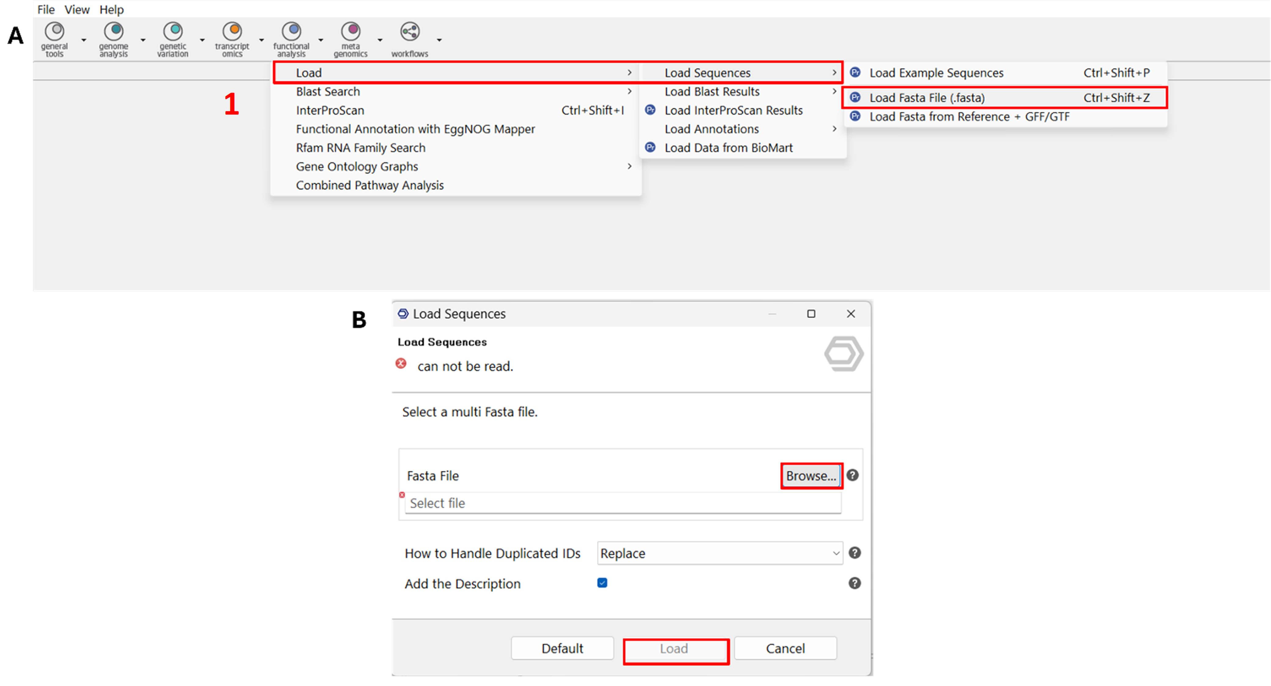
Figure 1. Screenshot showing the OmicsBox functional annotation workflow, specifically illustrating the upload of a multi-FASTA protein sequence file. (A) The interface displays the initial step of the annotation process, where the input dataset is selected for downstream functional annotation. (B) The selected dataset, shown as the multi-FASTA file, is now ready for processing in BLAST analysis. Label 1 is highlighted in red to indicate the first step in the workflow.
2. Run the Blast Search.
a. Navigate to Functional Analysis → Blast Search → Blast (Figure 2).
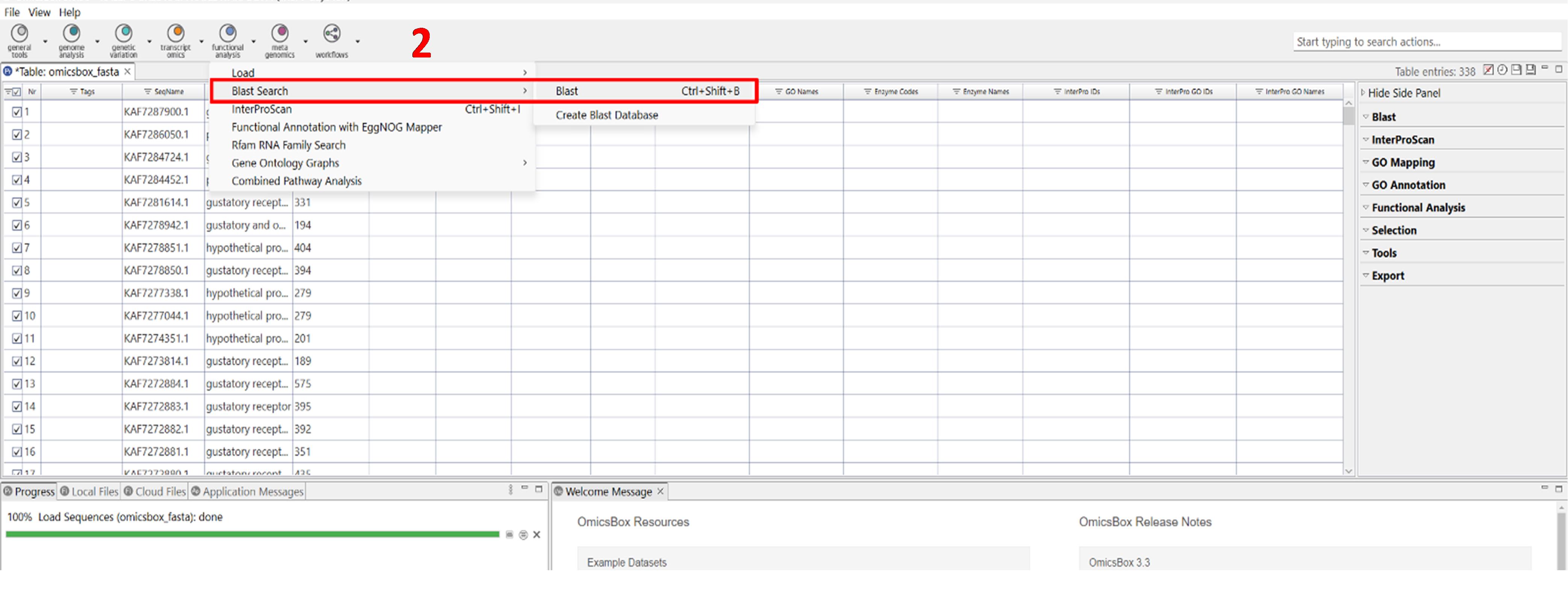
Figure 2. Screenshot showing the location of the BLAST tool within the Functional Analysis module of OmicsBox. The interface highlights the exact position of the BLAST tool, which is used for performing sequence similarity searches as part of the functional annotation process. Label 2 is highlighted in red to indicate the second step in the workflow.
b. Select NCBI Blast - online and click Next (Figure 3A).
c. Choose the non-redundant (nr) protein database with blastp (Figure 3B).
d. Set the E-value threshold to 1.0E-3 and limit the number of hits to 10 per query (Figure 3B).
e. Accept the default settings, specify the output directory, and click Run (Figure 3C, D).
Representative output: Each sequence is labelled BLASTED and highlighted in orange after processing.
Note: The duration of this step depends on the number and length of input sequences.
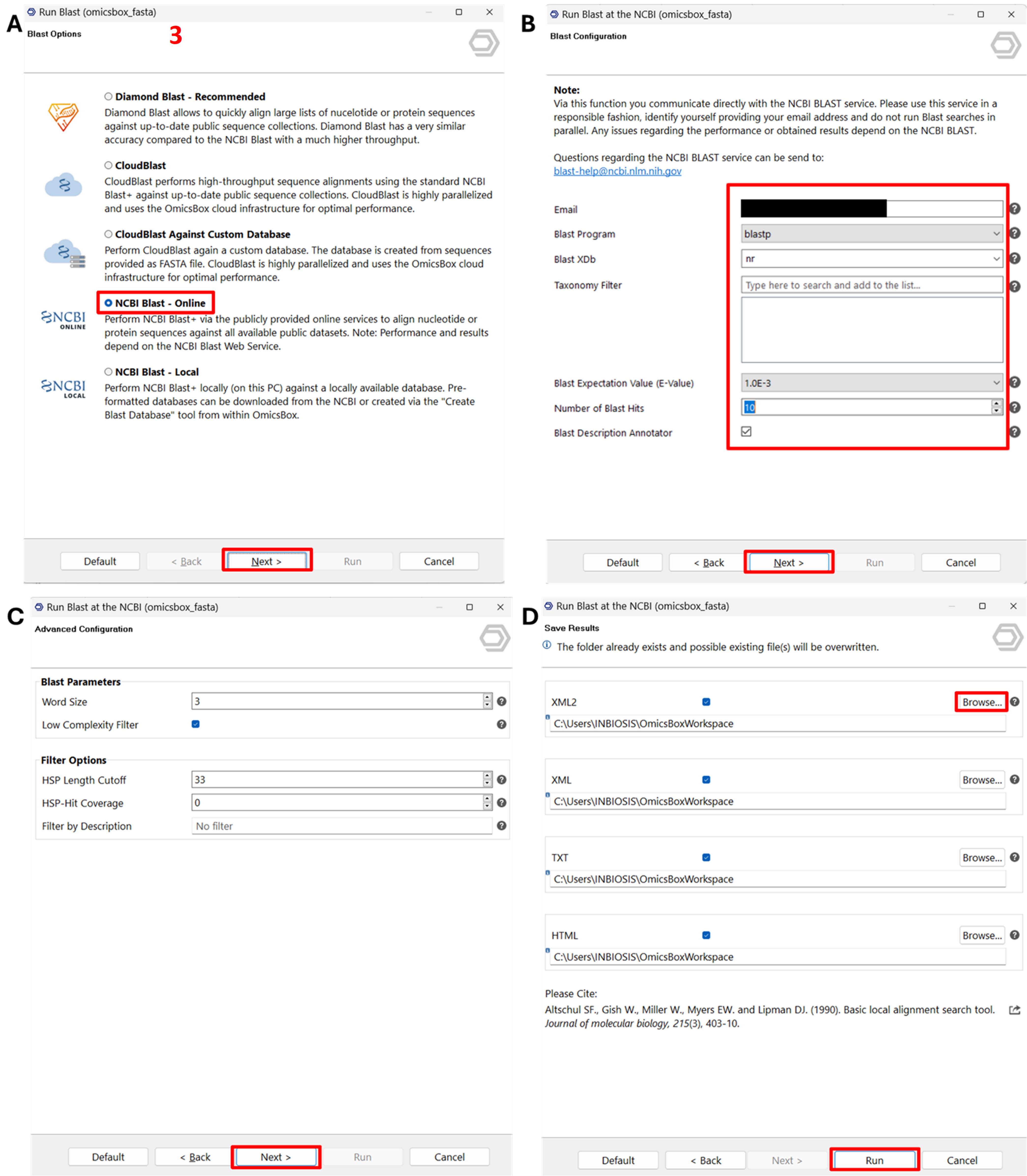
Figure 3. Screenshot illustrating the steps to run BLAST within the Functional Analysis module of OmicsBox. (A) Selection of input sequences for BLAST analysis, specifying the dataset to be processed. (B) Configuration of BLAST search parameters, including database selection and e-value threshold settings. (C) Additional options for customising the BLAST search to refine sequence similarity results. (D) Initiation of the BLAST process, starting the sequence alignment against reference databases for functional annotation. Label 3 is highlighted in red to indicate the third step in the workflow.
3. Run InterProScan for Domain Analysis.
a. Go to Functional Analysis → InterProScan.
b. Select EMBL-EBI InterPro and click Next (Figure 4A).
c. Accept the default settings and proceed through the Next steps (Figure 4B, C).
d. Choose an output folder and click Run (Figure 4D).
Representative output: Annotated sequences are tagged INTERPRO and coloured pink.
Note: This step may take time depending on the dataset size and internet speed.
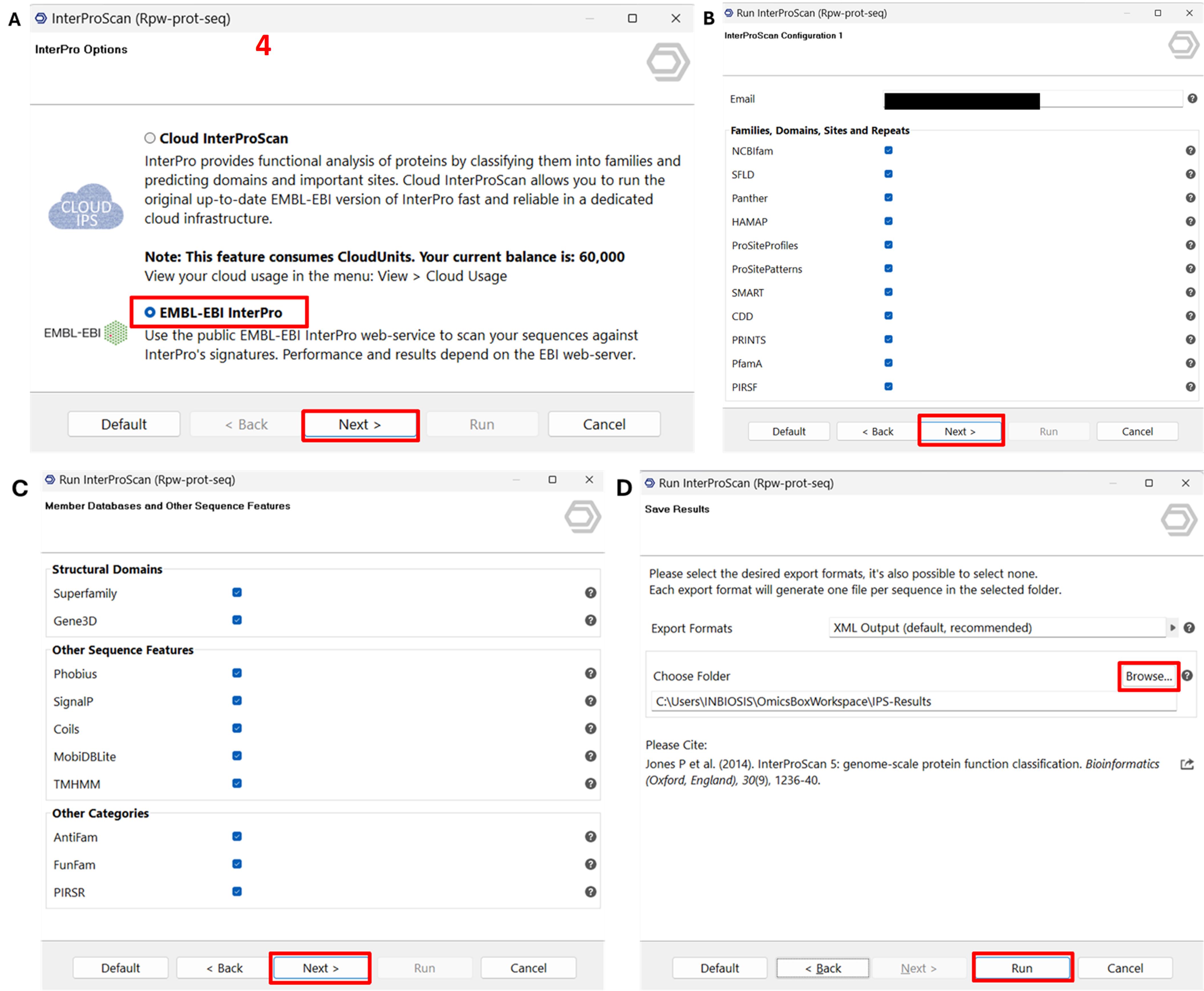
Figure 4. Screenshot illustrating the steps to run InterProScan in OmicsBox for domain analysis of protein sequences. (A) Selection of protein input files for InterProScan analysis. (B) Choice of relevant databases for identifying conserved domains and functional motifs. (C) Configuration of additional options for customising the scan. (D) Initiation of the InterProScan process to perform domain analysis and retrieve annotation results. Label 4 is highlighted in red to indicate the fourth step in the workflow.
4. Map GO terms (Figure 5).
a. In the right-side panel, locate GO Mapping.
b. Click the blue Pr icon to open the GOA version window.
c. Click Run to begin GO term mapping.
Representative output: Mapped sequences are labelled MAPPED and shown in green.
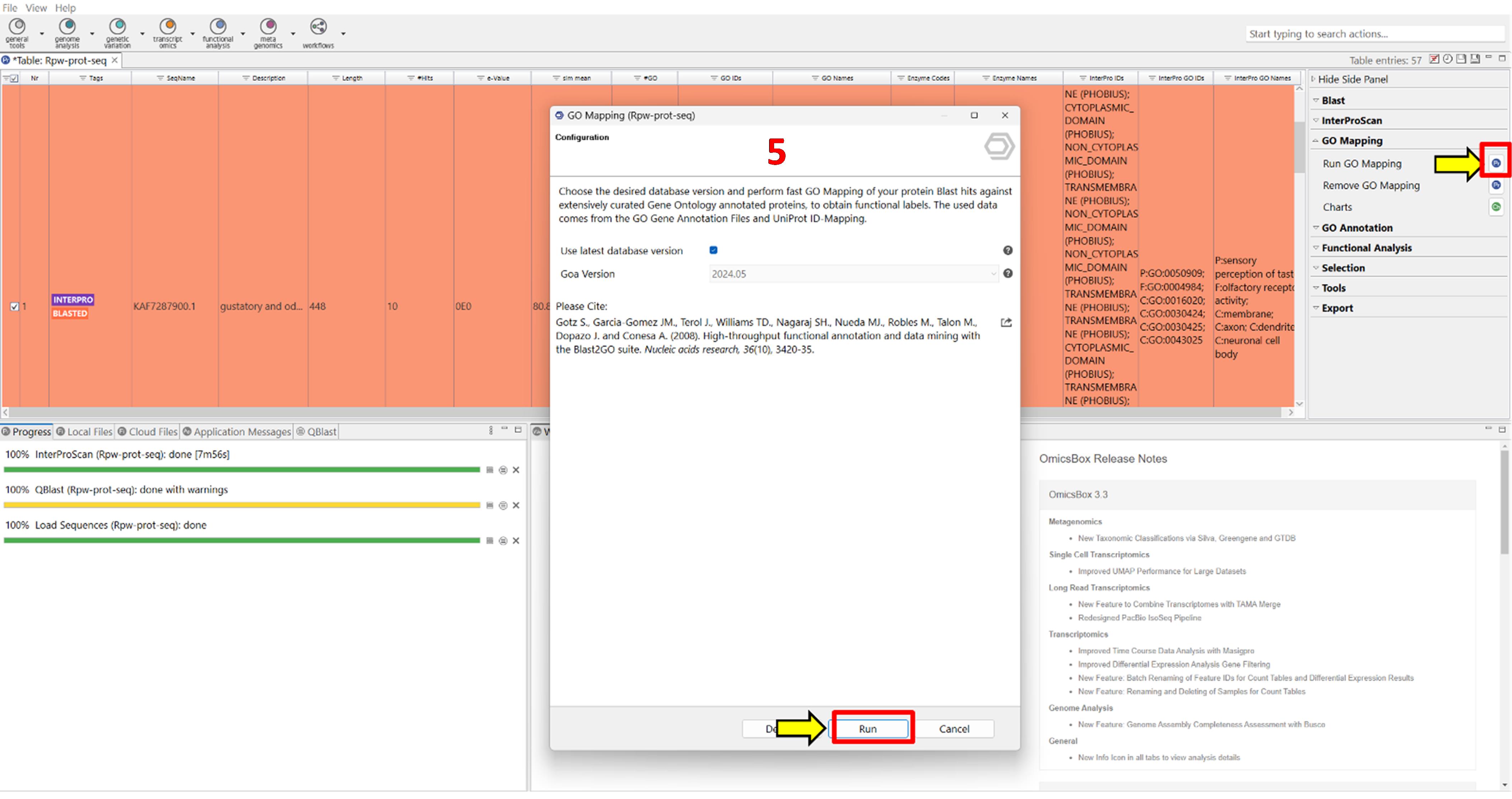
Figure 5. Screenshot illustrating the single-step process to run gene ontology (GO) mapping in OmicsBox for assigning GO terms to protein sequences. The interface shows the selection of protein sequences, and the assignment of GO terms based on BLAST hits against curated databases, facilitating functional interpretation of the sequences. Label 5 is highlighted in red to indicate the fifth step in the workflow.
5. Annotate GO terms (Figure 6).
a. Click GO Annotation in the right-side panel.
b. Proceed with the default settings and click Run.
Representative output: Annotated sequences are labelled ANNOTATED and appear in blue.
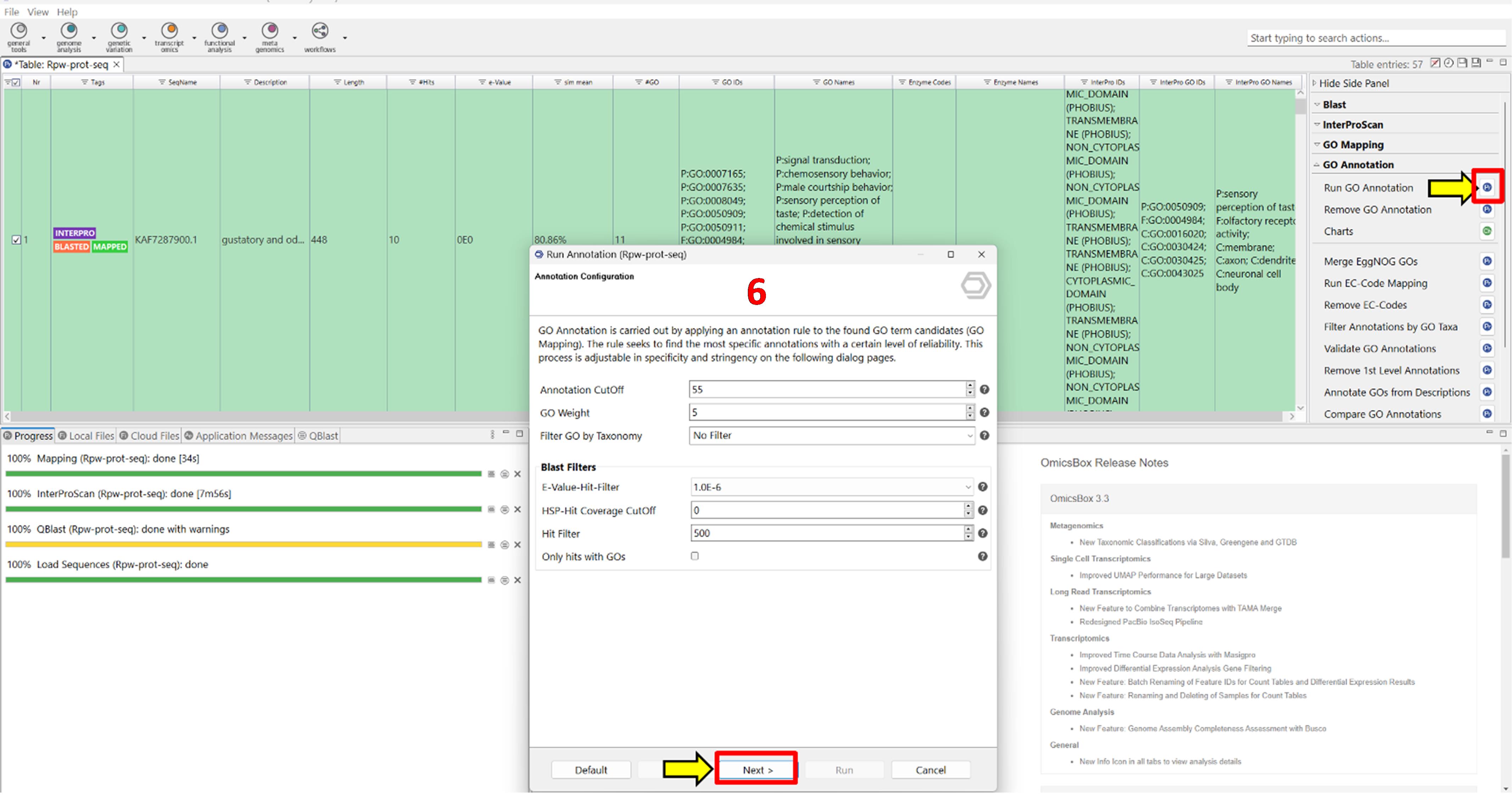
Figure 6. Screenshot showing the gene ontology (GO) annotation step in OmicsBox. The interface illustrates the assignment of functional terms to proteins based on mapped GO categories, providing insights into biological processes, cellular components, and molecular functions associated with the annotated sequences. Label 6 is highlighted in red to indicate the sixth step in the workflow.
6. Generate GO charts (Figure 7).
a. Under GO Annotation, click Charts.
b. Enable the following options:
• GO distribution by level.
• Direct GO count (select all three GO categories: Molecular Function, Biological Process, and Cellular Component).
c. Save the generated charts to the working directory.
Representative output: Bar charts showing GO term distributions across categories.
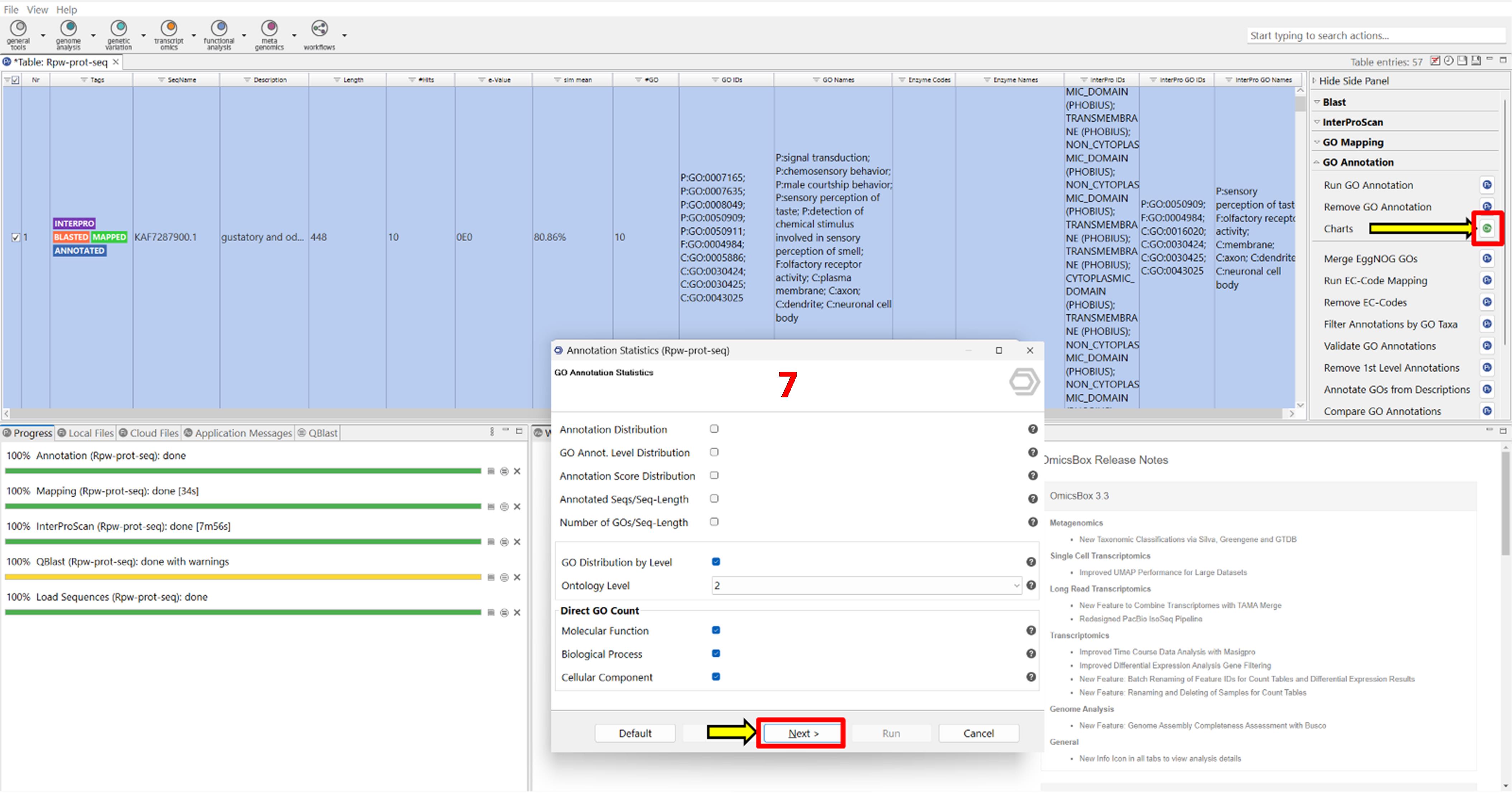
Figure 7. Screenshot showing the setup for generating gene ontology (GO) annotation statistics in OmicsBox. The interface displays options to select GO categories, including molecular function, biological process, and cellular component, allowing for examination of the functional attributes of annotated proteins. Label 7 is highlighted in red to indicate the seventh step in the workflow.
7. Export annotated data (Figure 8).
a. Click Export in the right-side panel and select Export Table.
b. Specify the output path and click Export.
c. To export additional files (e.g., GFF, GO annotations, mapping results, FASTA), click the blue Pr icon next to the respective export option, configure the settings, and click Export.
Note: Exported files can be used for downstream analyses such as enrichment, visualisation, or integration with other omics data.
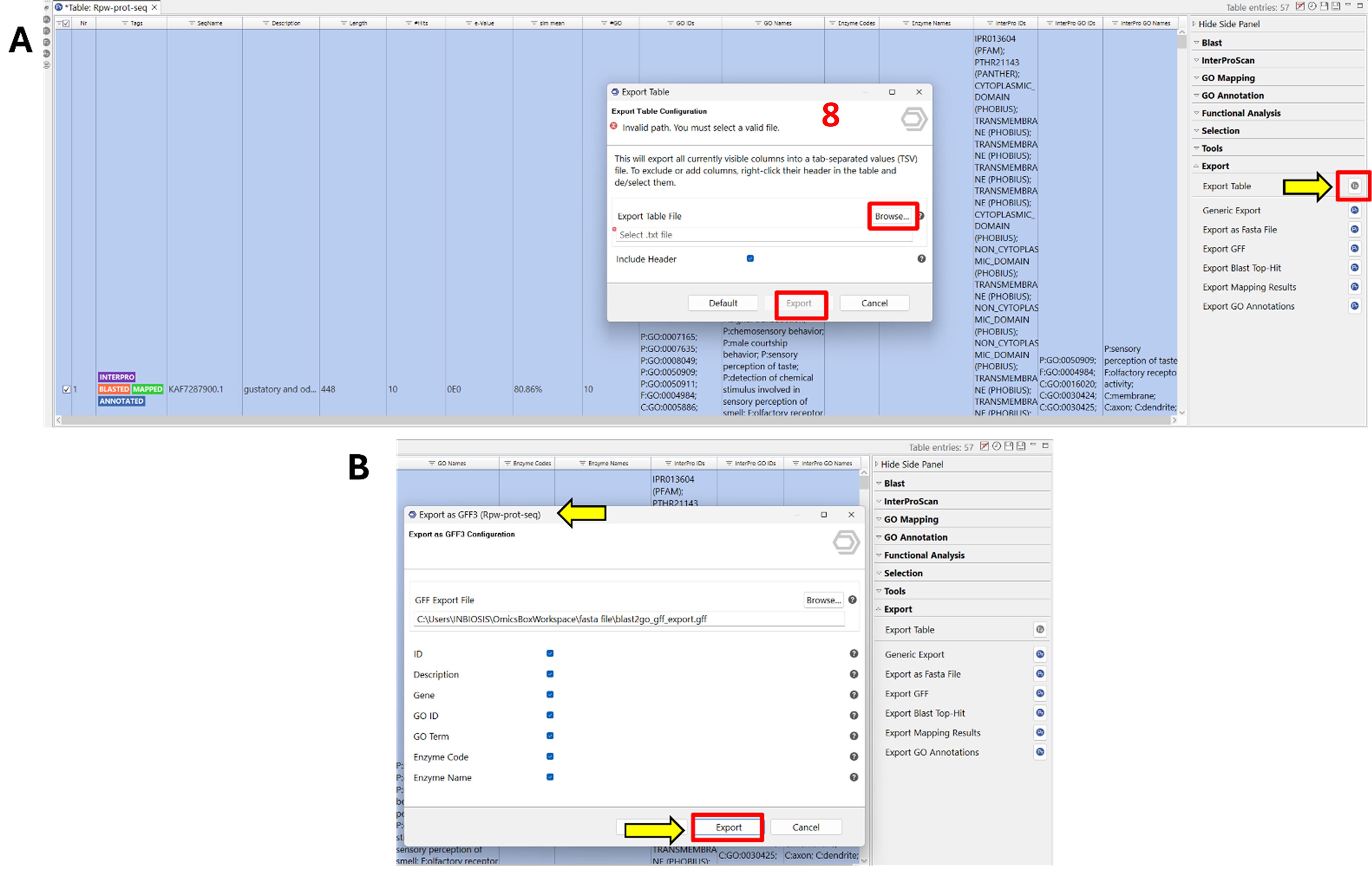
Figure 8. Screenshot showing the export of protein sequences along with annotated information, including InterProScan domain regions and gene ontology (GO) terms. (A) Interface for selecting export options, including annotated protein sequences and associated functional data. (B) Display of exported content, providing a detailed overview of protein function and domain structure for downstream analysis. Label 8 is highlighted in red to indicate the eighth step in the workflow.
D. Running LocalColabFold for protein structure prediction
This section describes the use of LocalColabFold v1.5.5 for predicting the 3D structures of GR proteins from RPW. LocalColabFold is a high-performance, locally executable version of AlphaFold2 that supports batch processing and GPU acceleration [9,14].
Note: For users without access to a local GPU, the web-based ColabFold v1.5.5 notebook is available at https://colab.research.google.com/github/sokrypton/ColabFold/blob/main/AlphaFold2.ipynb. However, it supports only single-sequence predictions.
1. Install LocalColabFold software on Linux.
Follow the installation instructions provided in the official LocalColabFold GitHub repository: https://github.com/YoshitakaMo/localcolabfold.
Note: The repository includes detailed steps for setting up the environment, installing dependencies, and configuring the system. Ensure your system meets the minimum requirements (Python ≥3.8, CUDA ≥11.1, GCC ≥9.0) and has a compatible GPU for optimal performance.
2. Prepare input FASTA files.
a. Use a Python script to split the multi-FASTA file into individual FASTA files.
b. Place the individual FASTA files in an input directory (e.g., single_files_dir).
c. Create an output directory (e.g., outputDir) to store prediction results.
Script location: Code S1 file (script 4: multi_to_single_fasta.py).
Command to run the script:
python3 multi_to_single_fasta.pyNote: The script uses Biopython [11] and is compatible with Python 3.
3. Run structure prediction (Figure 9).
a. Execute the following command in the Linux terminal:
colabfold_batch --templates --amber --use-gpu-relax /home/Documents/colab/single_files_dir /home/Documents/colab/outputDir/b. The --templates flag enables template-based modelling.
c. The --amber and --use-gpu-relax flags apply energy minimisation using Amber force fields.
Representative output: For each input sequence, ColabFold generates five ranked models (PDB files), including relaxed and unrelaxed versions.
Note: Only relaxed models are used for downstream analysis due to their improved physical accuracy and structural stability.
Figure 9. Screenshot showing the execution of LocalColabFold in a Linux terminal. The interface displays the command line process for running LocalColabFold, which is used for protein structure prediction.
4. Analyse ColabFold output files.
a. Navigate to the output directory to access predicted structures.
b. For each protein, identify the rank 1 relaxed model for further analysis.
Note: Rank 1 models typically represent the most accurate predictions [15].
5. Extract quality metrics using Python.
a. Use a Python script to parse JSON files and extract pLDDT, PAE, and pTM values.
b. Compute the average pLDDT and maximum PAE for each model.
c. Save the results in a CSV file for downstream analysis.
Script location: Code S1 file (script 5: process_json_to_csv.py).
Command to run the script:
python3 process_json_to_csv.pyNote: This automated approach enables scalable evaluation of large protein datasets.
Data analysis
Result interpretation
A total of 113 GR protein sequences were initially collected for R. ferrugineus, including 60 sequences retrieved from literature [6], 11 from the NCBI database, and 42 from UniProt. After merging all retrieved sequences into a single multi-FASTA file, preprocessing steps were applied to ensure data quality. Eleven redundant sequences were identified and filtered using a custom Python script based on sequences and accession numbers. Seven partial sequences were excluded using a custom Python script that identifies entries lacking complete open reading frames or essential domain features. As a result, 95 unique full-length GR sequences were retained for further analysis.
Functional annotation of 95 protein sequences revealed their involvement in diverse biological processes, molecular activities, and cellular components, categorised under GO terms (Figure 10, Dataset S4). The biological roles for these GRs included sensory perception of taste (40), male courtship (28), chemosensory behaviour (25), and signal transduction (23). Notably, in molecular functions, 17 proteins displayed sweet taste receptor activity. In the cellular component, neuronal cell bodies and dendrites were enriched with 28 proteins each, highlighting the importance of these receptors in sensory signalling. These observations suggest that GRs in RPW play central roles in chemosensory-driven behaviours, consistent with functional conservation observed in model insects such as the fruit fly (D. melanogaster) [16].
Figure 10. Bar graph depicting the gene ontology (GO) terms assigned to gustatory receptor (GR) sequences in R. ferrugineus. The graph shows the distribution of GO terms across three categories: biological process (red), molecular function (blue), and cellular component (green). The numbers on the bars represent the count of protein sequences associated with each GO term category. This dataset reflects the GO annotations generated from functional analysis of the gustatory proteins.
Structural prediction using LocalColabFold generated five models per sequence, with top-ranked models selected based on pLDDT, pTM scores, and PAE values. The residue-level confidence is measured by the pLDDT score, which ranges from 0 to 100. The pTM ranges from 0 to 1 and estimates the accuracy of the overall protein fold. Higher scores in pLDDT and pTM indicate more reliability and precision in the predicted structural model. The PAE plot offers insights into the positional accuracy of predicted protein structures by visualising the expected error between residue pairs. Low PAE values (often represented by dark blue) indicate reliable residue positions and well-structured domains, while high PAE values (lighter colours) suggest uncertainty in those regions, often pointing to flexibility or disorder. For structural confidence, clear diagonal regions with low PAE values and high pLDDT scores suggest stable, well-folded domains, while off-diagonal regions reflect domain packing quality, with high PAE values indicating potential flexibility or uncertainty in domain orientation. Low pLDDT and high PAE regions, such as flexible loops, should be interpreted with caution, as they may correspond to dynamic, functionally key areas like ligand-binding sites. These regions could be further explored through molecular dynamics simulations to refine structural predictions and capture their dynamic behaviour.
The Rank 1 models from the LocalColabFold output, typically the most accurate [15], were chosen for further analysis. A strong positive correlation (Figure 11A) between pLDDT and pTM scores (r = 0.85, p < 0.05) confirmed the reliability of the predicted structures. High-confidence models (pLDDT ≥ 90) (Figure 11B) exhibited canonical seven-transmembrane helices, with intracellular N-terminals and extracellular C-terminals, enabling effective ligand binding and signal transduction. Moderate-confidence models (70 ≤ pLDDT < 90) were also included for comprehensive structural insights, whereas low-confidence models (pLDDT < 50) were excluded from functional interpretations.
Figure 11. Protein structure prediction of gustatory receptor (GR) proteins in R. ferrugineus. (A) Scatterplot showing the correlation between the average pLDDT (predicted local distance difference test) and pTM (predicted template modelling) scores for GR protein structures. (B) Bar chart displaying GR protein structures predicted using AlphaFold, with colour-coding based on the AlphaFold prediction confidence scale (from dark blue for high-confidence to yellow for low-confidence).
To assess the reliability of the predicted RPW GR structures, a comparative structural analysis was performed against a known fruit fly (D. melanogaster) GR crystal structure. The RPW GR protein (NCBI ID: KAF7272883) was selected for comparative analysis due to its high-confidence AlphaFold2 prediction (pLDDT = 91.28), indicating a reliable 3D structure with complete seven-transmembrane helices and functional relevance in sweet taste perception. Structural comparison with the fruit fly (D. melanogaster) GR (PDB ID: 8ZE2) revealed an RMSD of 2.8 Å over 375 matched atom pairs and conserved secondary structure elements (Figure 12A), confirming the accuracy of the predicted model. These conserved motifs suggest similar ligand-binding and signalling functions, validating the in silico modelling pipeline and supporting the evolutionary conservation of GR-mediated chemosensory processes. The ribbon models of RPW GR (red) and fruit fly (D. melanogaster) GR (blue) demonstrate high alignment, with well-conserved secondary structure elements across both proteins. Additionally, sequence alignment (Figure 12B) highlights conserved residues critical for protein function, further supporting the structural integrity of the modelled RPW GR. The low RMSD and conserved secondary structure elements indicate that the predicted RPW GR retains essential structural folds [17]. In the absence of crystal structures for coleopteran GRs, this study demonstrates that in silico approaches can effectively bridge the gap in structural understanding across insect species.
Figure 12. Gustatory receptor (GR) protein structure comparison. (A) Visual comparison of fruit fly (D. melanogaster) GR (PDB ID: 8ZE2 [18], shown in blue) with red palm weevil (R. ferrugineus) GR (NCBI ID: KAF7272883, shown in red), aligned with ChimeraX [19]. (B) Structural alignment between two protein structures, showing conserved residues across the aligned regions. The alignment highlights conserved positions (marked in red) that are maintained in both protein structures, with the colour-coded representation indicating the level of conservation across the sequences.
In conclusion, this study presents a robust computational framework integrating OmicsBox-based sequence annotation with ColabFold-driven structure prediction to identify and characterise GR proteins in RPW. Functional annotation highlighted their roles in signalling, chemosensory behaviour, and sensory perception, while sequence analysis confirmed membrane localisation and provided functional gene ontology terms for hypothetical proteins. High-confidence 3D structures were generated, supported by pLDDT and pTM scores, and comparative structural analysis with the fruit fly (D. melanogaster) GR crystal structure confirmed evolutionary conservation of GR motifs. Among these, the RPW GR protein KAF7272883 was shortlisted as the most reliable model. This flexible, reproducible pipeline demonstrates broad applicability for studying chemosensory proteins in non-model insects. Future directions include incorporating docking and molecular dynamics simulations to provide insights into protein–ligand interactions and dynamic stability, thereby advancing understanding of chemosensory mechanisms and aiding the development of targeted pest control strategies.
Validation of protocol
To ensure the reliability and reproducibility of our computational pipeline, we validated it using fruit fly (D. melanogaster) GR proteins. A total of 1,443 GR protein sequences were retrieved from the NCBI protein database. After preprocessing steps, including the removal of 1,158 redundant sequences and 182 partial sequences, a final dataset of 103 full-length, non-redundant GR sequences was obtained for downstream analyses. Functional annotation of these sequences using OmicsBox revealed that most GR proteins are associated with key biological functions, such as ion transmembrane transport, signal transduction, and the detection of chemical stimuli involved in the sensory perception of sweet taste. The predominant molecular functions included sweet taste receptor activity and ligand-gated monoatomic ion channel activity, while the main cellular component was the plasma membrane (Dataset S5). These findings are consistent with the known roles of GR proteins in chemosensory signalling and provide a biologically relevant foundation for structural modelling.
All 103 GR proteins were structurally modelled using LocalColabFold. Of these, 97 structures were predicted with high confidence, reflected by average pLDDT scores above 70. In AlphaFold2, pLDDT scores greater than 70 indicate well-resolved secondary structures, and scores above 90 suggest near-experimental accuracy [14,20]. To further evaluate structural reliability, the predicted model for one representative GR protein was compared to the experimentally resolved structure of fruit fly (D. melanogaster) GR (PDB ID: 8ZE2 [18]). The local RMSD between predicted and experimental structures was 1.29 Å (Figure 13), confirming high structural accuracy. These RMSD values are consistent with previous validation studies demonstrating that AlphaFold2 models achieve close agreement with crystal structures. Additionally, the pTM score, which quantifies global structural similarity and confidence in domain organisation, was assessed. pTM scores above 0.7 are indicative of reliable domain packing and overall structural fidelity, further supporting the robustness of the predicted GR models. This validation confirms that our pipeline can accurately translate sequence-level information into reliable 3D protein structures, even for proteins without experimentally resolved templates. Overall, these results demonstrate that the computational pipeline effectively integrates sequence retrieval and preprocessing, functional annotation, and structure prediction. The protocol produces reproducible and biologically meaningful results and is adaptable for investigating chemosensory GR proteins across diverse insect species beyond RPW.
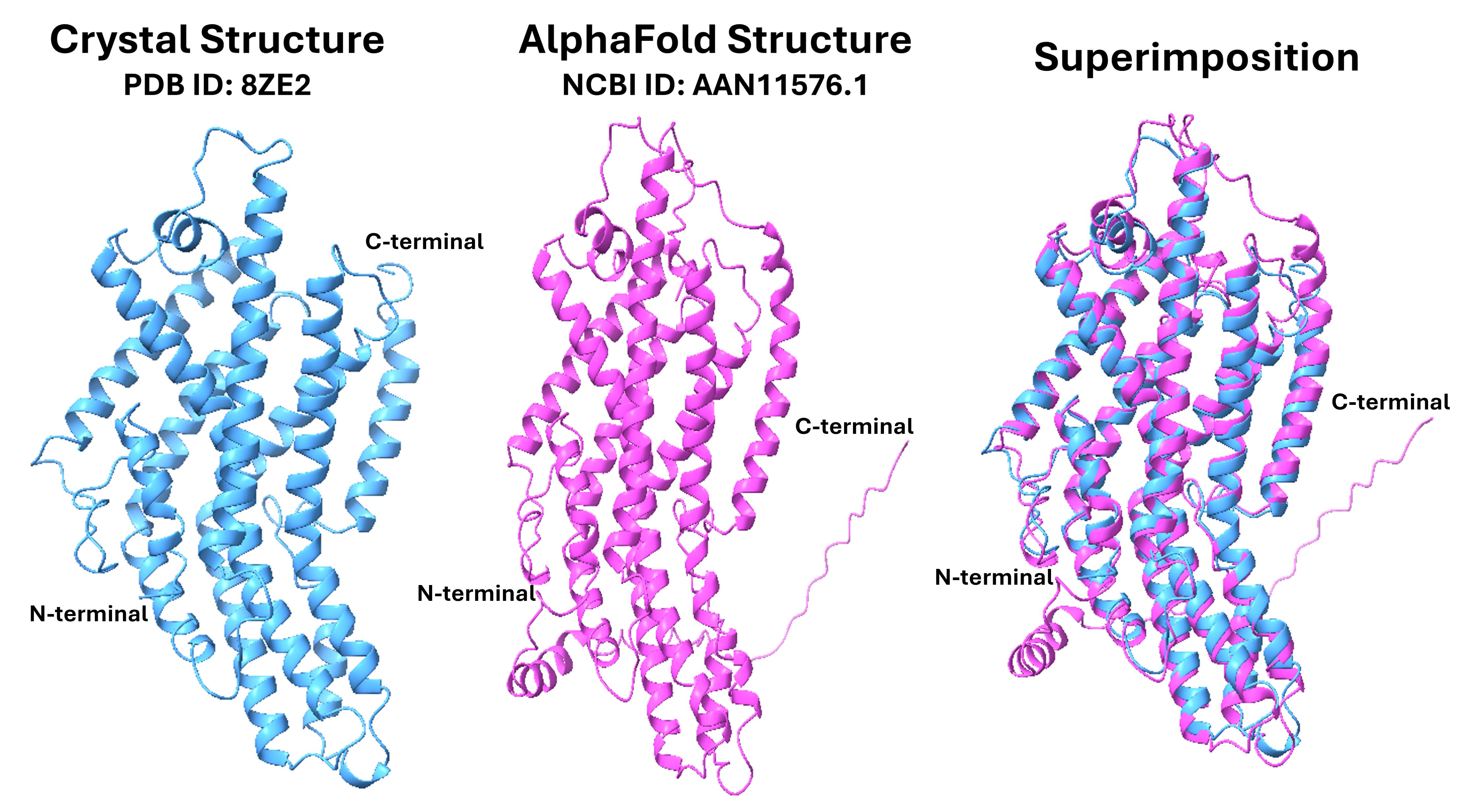
Figure 13. Superimposition of the crystal structure of the gustatory receptor (GR) for sugar taste 64a (PDB ID: 8ZE2 [18]), shown in blue) with the AlphaFold-modelled structure (NCBI ID: AAN11576.1, shown in magenta). This comparison highlights the structural alignment between experimental and predicted models of the receptor.
This protocol (or parts of it) has been used and validated in the following research article:
• Rajeswari Kalepu, Maizom Hassan, Azzmer Azzar Abdul Hamid, et al. [21]. Unveiling Key Olfactory Receptors in Rhynchophorus ferrugineus Red Palm Weevil: A High-Throughput Structural Bioinformatics Approach. Authorea. June 18, 2025. DOI: 10.22541/au.175028961.14336860/v1 (Figure 1, panels 1–2)
Reproducibility
The successful validation of this pipeline in D. melanogaster demonstrates its robustness and adaptability across different species. Despite variations in sequence diversity and structural complexity, the pipeline consistently provided reliable functional annotation and high-confidence structural models. This confirms its potential for application in other insect species, particularly those with limited experimental structural data. Furthermore, the methodology is not restricted to GR proteins; it can be extended to study other chemosensory proteins, such as odorant receptors, ionotropic receptors, odorant-binding proteins, and chemosensory proteins, across various agricultural and ecological pests. Its versatility makes it an effective tool for studying protein–ligand interactions, chemosensory mechanisms, and identifying new molecular targets in insect pests.
General notes and troubleshooting
General notes
1. Applicability to other species: Although this approach was initially created for GR proteins from RPW, it can be modified to analyse protein sequences from other species, such as a variety of receptor types and other protein families.
2. Data quality and preprocessing: The accuracy of functional annotation and structural modelling depends on the quality and completeness of input sequences. Redundant or partial sequences should be carefully removed to avoid errors in downstream analysis.
3. Functional annotation variability: Gene ontology annotations depend on available databases and homology information. In poorly annotated species, annotations may be incomplete, which could affect downstream functional interpretation.
4. Structural modelling limitations: AlphaFold2/ColabFold predictions are highly reliable for well-conserved protein regions, but low-confidence regions (pLDDT < 70) may correspond to disordered segments or poorly conserved domains. These regions should be interpreted cautiously.
5. Computational resources: Structural modelling and large-scale functional annotation require sufficient computational power, especially for large protein datasets. Using GPUs and optimised software versions can significantly reduce computation time.
6. Integration with downstream analyses: Predicted structures can be used for molecular docking, virtual screening, or molecular dynamics simulations. Models should meet high confidence thresholds (pLDDT ≥ 70) before further application.
Troubleshooting
Problem 1: Low-quality or incomplete protein sequences.
Possible cause: Sequences retrieved from databases may be partial, truncated, or contain errors.
Solutions: Perform thorough preprocessing to remove redundant or partial sequences before downstream analysis. Use sequence length filters and verify annotations against trusted databases like NCBI or UniProt.
Problem 2: Functional annotation yields few or no GO terms.
Possible causes: The input protein may lack homology to well-annotated proteins, or the database used may be incomplete.
Solutions: Update annotation databases to the latest version. Consider using multiple annotation tools to cross-validate results (e.g., PANTHER).
Problem 3: Long computation times or software errors during modelling.
Possible causes: Large dataset size, limited computational resources, or software incompatibility.
Solutions: Use GPU acceleration if available, reduce batch sizes, or split the dataset into smaller subsets. Ensure software and dependencies are correctly installed and updated.
Supplementary information
The following supporting information can be downloaded here:
1. Dataset S1. Input file for RPW GR protein sequences in Fasta format.
2. Dataset S2. Following preprocessing, the output file for RPW GR protein sequences is in Fasta format.
3. Dataset S3. OmicsBox Functional Annotation Workflow. Video shows the step-by-step demonstration of functional annotation analysis using OmicsBox V3.4. This video provides a walkthrough of the key steps involved in performing functional annotation with OmicsBox V3.4, using a small dataset for demonstration purposes.
4. Dataset S4. RPW GR interpretation data.
5. Dataset S5. D. melanogaster validation data.
6. Code S1. Custom Python scripts.
Acknowledgments
Specific contributions of each author:
Rajeswari Kalepu: Conceptualization, Writing—Original Draft, Writing—Review & Editing.
Azzmer Azzar Abdul Hamid: Conceptualization, Investigation, Supervision, Writing—Review & Editing.
Maizom Hassan: Investigation, Supervision, Writing—Review & Editing.
Norfarhan Mohd-Assaad: Investigation, Supervision, Writing—Review & Editing.
Nor Azlan Nor Muhammad: Supervision, Investigation, Conceptualization, Writing—Review & Editing, Funding acquisition.
This research was funded by Universiti Kebangsaan Malaysia through the Geran Universiti Penyelidikan (GUP), grant number GUP-2021-068.
This protocol is based on the author’s original research, currently available as a preprint: 10.22541/au.175028961.14336860/v1.
Competing interests
The authors declare no conflicts of interest.
References
- Antony, B., Soffan, A., Jakše, J., Abdelazim, M. M., Aldosari, S. A., Aldawood, A. S. and Pain, A. (2016). Identification of the genes involved in odorant reception and detection in the palm weevil Rhynchophorus ferrugineus, an important quarantine pest, by antennal transcriptome analysis. BMC Genomic. 17(1): 1–22. https://doi.org/10.1186/s12864-016-2362-6
- Venthur, H., Arias, I., Lizana, P., Jakše, J., Alharbi, H. A., Alsaleh, M. A., Pain, A. and Antony, B. (2023). Red palm weevil olfactory proteins annotated from the rostrum provide insights into the essential role in chemosensation and chemoreception. Front Ecol Evol. 11: e1159142. https://doi.org/10.3389/fevo.2023.1159142
- Kurdi, H., Al-Aldawsari, A., Al-Turaiki, I. and Aldawood, A. S. (2021). Early Detection of Red Palm Weevil, Rhynchophorus ferrugineus (Olivier), Infestation Using Data Mining. Plants. 10(1): 95. https://doi.org/10.3390/plants10010095
- Faleiro, J. R. (2006). A review of the issues and management of the red palm weevil Rhynchophorus ferrugineus (Coleoptera: Rhynchophoridae) in coconut and date palm during the last one hundred years. Int J Trop Insect Sci. 26(3): 135–154. https://doi.org/10.1079/IJT2006113
- Ahmad, J. N., Manzoor, M., Aslam, Z. and Nazeer Ahmad, S. J. (2020). Molecular study on field evolved resistance of red palm weevil (Rhynchophorus ferruginous) and its management through RNAi. Pak J Zool. 52(2): 477–486. https://doi.org/10.17582/journal.pjz/20190105110153
- Engsontia, P. and Satasook, C. (2021). Genome-Wide Identification of the Gustatory Receptor Gene Family of the Invasive Pest, Red Palm Weevil, Rhynchophorus ferrugineus (Olivier, 1790). Insects. 12(7): 611. https://doi.org/10.3390/insects12070611
- Gonzalez, F., Johny, J., Walker, W. B., Guan, Q., Mfarrej, S., Jakše, J., Montagné, N., Jacquin-Joly, E., Alqarni, A. A., Al-Saleh, M. A., et al. (2021). Antennal transcriptome sequencing and identification of candidate chemoreceptor proteins from an invasive pest, the American palm weevil, Rhynchophorus palmarum. Sci Rep. 11(1): 1–14. https://doi.org/10.1038/s41598-021-87348-y
- Götz, S., García-Gómez, J. M., Terol, J., Williams, T. D., Nagaraj, S. H., Nueda, M. J., Robles, M., Talón, M., Dopazo, J. and Conesa, A. (2008). High-throughput functional annotation and data mining with the Blast2GO suite. Nucleic Acids Res. 36(10): 3420–3435. https://doi.org/10.1093/NAR/GKN176
- Mirdita, M., Schütze, K., Moriwaki, Y., Heo, L., Ovchinnikov, S. and Steinegger, M. (2022). ColabFold: making protein folding accessible to all. Nat Methods. 19(6): 679–682. https://doi.org/10.1038/s41592-022-01488-1
- Prajapati, M. R., Kumar, P., Pratap Singh, R., Shanker, R., Singh, J., Kumar Bharti, M., Singh, R., Verma, H., Gangwar, L., Singh Gaurav, S., et al. (2024). De novo transcriptome assembly, annotation and SSR mining data of Hellula undalis (Fabr.) (Lepidoptera: Pyralidae), the cabbage webworm. J Genet Eng Biotechnol. 22(3): 100393. https://doi.org/10.1016/j.jgeb.2024.100393
- Cohen, Z. P., Perkin, L. C., Sim, S. B., Stahlke, A. R., Geib, S. M., Childers, A. K., Smith, T. P. L. and Suh, C. (2023). Insight into weevil biology from a reference quality genome of the boll weevil, Anthonomus grandis grandis Boheman (Coleoptera: Curculionidae). G3. 13(2): e1093/g3journal/jkac309. https://doi.org/10.1093/g3journal/jkac309
- Diaz-Vidal, T., Martínez-Pérez, R. B. and Rosales-Rivera, L. C. (2023). Computational insights of the molecular recognition between volatile molecules and odorant binding proteins from the red palm weevilRhynchophorus ferrugineus. J Biomol Struct Dyn. 42(20): 11285–11298. https://doi.org/10.1080/07391102.2023.2262583
- Cock, P. J. A., Antao, T., Chang, J. T., Chapman, B. A., Cox, C. J., Dalke, A., Friedberg, I., Hamelryck, T., Kauff, F., Wilczynski, B., et al. (2009). Biopython: freely available Python tools for computational molecular biology and bioinformatics. Bioinformatics. 25(11): 1422. https://doi.org/10.1093/BIOINFORMATICS/BTP163
- Jumper, J., Evans, R., Pritzel, A., Green, T., Figurnov, M., Ronneberger, O., Tunyasuvunakool, K., Bates, R., Žídek, A., Potapenko, A., et al. (2021). Highly accurate protein structure prediction with AlphaFold. Nature. 596(7873): 583–589. https://doi.org/10.1038/s41586-021-03819-2
- Yin, R., Feng, B. Y., Varshney, A. and Pierce, B. G. (2022). BenchmarkingAlphaFoldfor protein complex modeling reveals accuracy determinants. Protein Sci. 31(8): e4379. https://doi.org/10.1002/pro.4379
- Arntsen, C., Guillemin, J., Audette, K. and Stanley, M. (2024). Tastant-receptor interactions: insights from the fruit fly. Front Nutr. 11: e1394697. https://doi.org/10.3389/fnut.2024.1394697
- Arnce, L. R., Bubnell, J. E. and Aquadro, C. F. (2025). Comparative Analysis of Drosophila Bam and Bgcn Sequences and Predicted Protein Structural Evolution. J Mol Evol. 93(2): 278–291. https://doi.org/10.1007/s00239-025-10245-9
- Chen, R., Zhang, R., Li, L., Wang, B., Gao, Z., Liu, F., Chen, Y., Tian, Y., Li, B. and Chen, Q. (2024). Structure basis for sugar specificity of gustatory receptors in insects. Cell Discov. 10(1): 83. https://doi.org/10.1038/S41421-024-00716-6
- Meng, E. C., Goddard, T. D., Pettersen, E. F., Couch, G. S., Pearson, Z. J., Morris, J. H. and Ferrin, T. E. (2023). UCSF ChimeraX: Tools for structure building and analysis. Protein Sci. 32(11): e4792. https://doi.org/10.1002/PRO.4792
- Varadi, M., Anyango, S., Deshpande, M., Nair, S., Natassia, C., Yordanova, G., Yuan, D., Stroe, O., Wood, G., Laydon, A., et al. (2022). AlphaFold Protein Structure Database: massively expanding the structural coverage of protein-sequence space with high-accuracy models. Nucleic Acids Res. 50(D1): D439. https://doi.org/10.1093/NAR/GKAB1061
- Rajeswari Kalepu, Maizom Hassan, Azzmer Azzar Abdul Hamid, et al. (2025). Unveiling Key Olfactory Receptors in Rhynchophorus ferrugineus Red Palm Weevil: A High-Throughput Structural Bioinformatics Approach. Authorea. https://doi.org/10.22541/au.175028961.14336860/v1
Article Information
Publication history
Received: Aug 25, 2025
Accepted: Oct 14, 2025
Available online: Nov 6, 2025
Published: Nov 20, 2025
Copyright
© 2025 The Author(s); This is an open access article under the CC BY-NC license (https://creativecommons.org/licenses/by-nc/4.0/).
How to cite
Kalepu, R., Hamid, A. A. A., Hassan, M., Mohd-Assaad, N. and Muhammad, N. A. N. (2025). A Step-by-Step Computational Protocol for Functional Annotation and Structural Modelling of Insect Chemosensory Proteins. Bio-protocol 15(22): e5523. DOI: 10.21769/BioProtoc.5523.
Category
Bioinformatics and Computational Biology
Biochemistry > Protein > Structure
Environmental science > Plant > Plant-insect interaction
Do you have any questions about this protocol?
Post your question to gather feedback from the community. We will also invite the authors of this article to respond.