- Protocols

- Articles and Issues
- For Authors
- About
- Become a Reviewer

A Computational Workflow for Membrane Protein–Ligand Interaction Studies: Focus on α5-Containing GABA (A) Receptors

Published: Vol 15, Iss 22, Nov 20, 2025 DOI: 10.21769/BioProtoc.5515 Views: 2123
Reviewed by: Anonymous reviewer(s)
Original research article
The authors used this protocol in:

Oct 2025

Protocol Collections
Comprehensive collections of detailed, peer-reviewed protocols focusing on specific topics


Related protocols
Abstract
In neuropharmacology and drug development, in silico methods have become increasingly vital, particularly for studying receptor–ligand interactions at the molecular level. Membrane proteins such as GABA (A) receptors play a central role in neuronal signaling and are key targets for therapeutic intervention. While experimental techniques like electrophysiology and radioligand binding provide valuable functional data, they often fall short in resolving the structural complexity of membrane proteins and can be time-consuming, costly, and inaccessible in many research settings. This study presents a comprehensive computational workflow for investigating membrane protein–ligand interactions, demonstrated using the GABA (A) receptor α5β2γ2 subtype and mitragynine, an alkaloid from Mitragyna speciosa (Kratom), as a case study. The protocol includes homology modeling of the receptor based on a high-resolution template, followed by structure optimization and validation. Ligand docking is then used to predict binding sites and affinities at known modulatory interfaces. Finally, molecular dynamics (MD) simulations assess the stability and conformational dynamics of receptor–ligand complexes over time. Overall, this workflow offers a robust, reproducible approach for structural analysis of membrane protein–ligand interactions, supporting early-stage drug discovery and mechanistic studies across diverse membrane protein targets.
Key features
• Applicable to diverse membrane proteins, including ion channels and G protein-coupled receptors (GPCRs), facilitating ligand interactions and dynamic behavior in biologically relevant environments.
• Supports the investigation of both natural and synthetic compounds targeting specific receptor subtypes within complex membrane systems.
• Combines homology modeling, molecular docking, and molecular dynamics simulations to deliver comprehensive structural and functional insights.
• Showcased with the GABA (A) α5β2γ2 receptor subtype and alkaloid from Mitragyna speciosa, with adaptability to a broad range of receptor–ligand systems.
Keywords: Membrane protein modelingGraphical overview
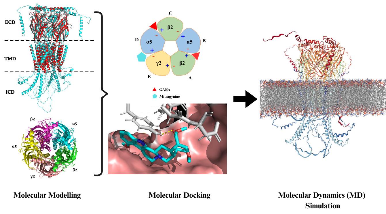
Comprehensive in silico methodological framework designed to investigate the molecular interactions between the alkaloid mitragynine and the α5β2γ2 subtype of the hippocampal GABA (A) receptor
Background
In the mammalian central nervous system (CNS), γ-aminobutyric acid (GABA) is the primary inhibitory neurotransmitter [1]. GABA (A) receptors are ionotropic receptors that, upon GABA binding, open chloride (Cl-) channels, leading to neuronal hyperpolarization and inhibition [2]. These receptors are pentameric ligand-gated ion channels, typically assembled from five subunits selected from 19 known types: α1–6, β1–3, γ1–3, δ, ε, θ, π, and ρ1–3 [3]. The most common brain configuration consists of two α, two β, and one additional subunit, forming αβγ or αβδ combinations, which correspond to synaptic and extrasynaptic receptors, respectively [4]. The specific subunit composition determines each receptor's pharmacological profile, regional brain distribution, and physiological role. Among the subunits, α5 is particularly notable for its involvement in cognitive processes, including learning and spatial memory [5–7]. The α5β2γ2 GABA (A) receptor subtype has been identified as a key modulator of cognition and anxiety-related behaviors. This receptor subtype is highly expressed in the hippocampus, particularly in the CA1 and CA3 regions, areas critical for memory encoding and spatial navigation [8,9]. Its anatomical localization and functional role make α5β2γ2 a compelling target for cognitive modulation. In this context, natural compounds with neuroactive properties may offer new avenues for modulating GABAergic signaling.
Mitragyna speciosa (commonly known as Kratom) is a tropical medicinal plant traditionally used for its stimulant and opioid-like effects [10]. Among its constituents, mitragynine is the primary and pharmacologically active alkaloid. Mitragynine exhibits analgesic, anti-inflammatory, and psychoactive properties [11], primarily acting as a partial agonist at the μ-opioid receptor and an antagonist at κ- and δ-opioid receptors [12]. Beyond its opioid-related activity, mitragynine has shown potential to interact with receptors involved in cognitive processes, raising interest in its neuromodulatory effects on GABAergic systems [13]. To systematically explore this potential, we developed an integrated in silico workflow to investigate the interaction of mitragynine with the α5β2γ2 GABA (A) receptor subtype. The protocol begins with homology modeling of the receptor using the α1β2γ2 subtype as a structural template. Following model optimization and validation, molecular docking is performed to predict mitragynine’s binding affinity and identify key interaction sites. Finally, molecular dynamics (MD) simulations are used to assess the stability and conformational behavior of the receptor–ligand complex. Overall, this computational approach provides detailed structural and dynamic insights into the potential neuromodulatory action of mitragynine on a cognitively significant GABA (A) receptor subtype.
Equipment
Hardware
For molecular docking and MD simulations, especially in in silico studies, access to adequate computational resources is essential for efficient performance. While the type or number of computing devices does not inherently affect the scientific validity or reproducibility of the results when using deterministic algorithms with identical parameters, it significantly impacts processing speed and overall throughput. In particular, parallel processing capabilities can greatly reduce simulation time and enhance workflow scalability. Suggested hardware specifications for an optimal workstation setup are summarized in Table 1.
Table 1. Specification summary of computing systems used in this study
| Specification | High-performance computer | Workstation custom PC |
| Model | Gigabyte Technology Co., Ltd. Z790 UD AX | Gigabyte Technology Co., Ltd. B550 AOROS ELITE |
| Processor type | Intel® CoreTM i9-14900K × 32 | AMD® Ryzen 5 5600x 6-core processor × 12 |
| Memory | 32 GB RAM | 32 GB RAM |
| Graphic processing unit (GPU) | NVIDIA GeForce RTX 4080/PCIe/SSE2/NVIDIA Corporation | NVIDIA Corporation GA106 [GeForce RTX 3060 Lite Hash Rate] |
| Disk capacity | 5.9 TB | 2.5 TB |
| Operating system | Ubuntu 22.04.5 LTS | Ubuntu 22.04.3 LTS |
Software and datasets
Software
This section provides an overview of the key software packages employed in the study, including molecular modeling platforms, simulation engines, and visualization tools, as summarized in Table 2.
Table 2. Summary of computational tools employed and their functional roles
| Software | Version | Function | References |
PyMOL | 2.5 | To display protein and ligand structures in 3D To allow molecular editing and measure distances, angles, and torsion between atoms and residues To render high-quality molecular graphics | [14] |
| MODELLER | 10.7 | To add missing residues To align the target sequences To generate 3D models of proteins by using the homologous structure as the template To rank and validate the quality of predicted models via the DOPE score | [15] |
| GROMACS | 2023.4 | To perform energy minimization and system equilibration To simulate protein complexes over time To analyze MD output | [16] |
| AutoDock Tools | 4.2 | To prepare ligand topology To assign partial charges to the protein To define a grid box over the target binding site | [17] |
| AutoDock Vina | 1.2.0 | To predict the binding poses and affinities of ligands To generate output files in PDBQT format | [18] |
| GRACE | 5.1.25 | To generate graphs To support overlaying multiple datasets for comparison | [19] |
| VMD | 1.9.4 | To load and playback MD simulation trajectories To generate high-quality molecular images and videos | [20] |
| Discovery Studio | 2021 | To analyze and visualize protein-ligand interactions in 2D and 3D | [21] |
Database and repositories
This section provides the validated and structured biological information required for each feature, as summarized in Table 3.
Table 3. Resources and databases utilized in structural and molecular analysis
| Name | Feature | URL |
| RCSB Protein Database (RCSB PDB) | Database for the three-dimensional structural data of large biological molecules such as proteins and nucleic acids | https://www.rcsb.org/ |
| UniProt | Database for protein sequences | https://www.uniprot.org/ |
| AlphaFold | Program for protein structure prediction | https://alphafold.ebi.ac.uk/ |
| Clustal Omega | Multiple sequence alignment programs | https://www.ebi.ac.uk/jdispatcher/msa/clustalo |
| Phylip to Pir sequence converter | Program for translation of the sequence alignment data between two formats | https://sequenceconversion.bugaco.com/converter/biology/sequences/pir_to_phylip.php |
| UCLA-DOE LAB | Verification of protein structures | https://saves.mbi.ucla.edu/ |
| CHARMM-GUI | Constructing coarse-grained, atomistic models, suitable for simulation, with a single or complex interest in solution or membrane settings | https://www.charmm-gui.org/ |
| PubChem | Database for chemical molecules | https://pubchem.ncbi.nlm.nih.gov/ |
| Protein Ligand Interaction Profiler (PLIP) | Identification of non-covalent interactions between biological macromolecules and ligands | https://plip-tool.biotec.tu-dresden.de/plip-web/plip/index |
File organization and directory setup
This section provides the structured directory information required across different stages of the in silico pipeline, as illustrated in Figure 1. Establishing a systematic folder hierarchy ensures proper file management, reproducibility, and efficient access to input, output, and analysis files.
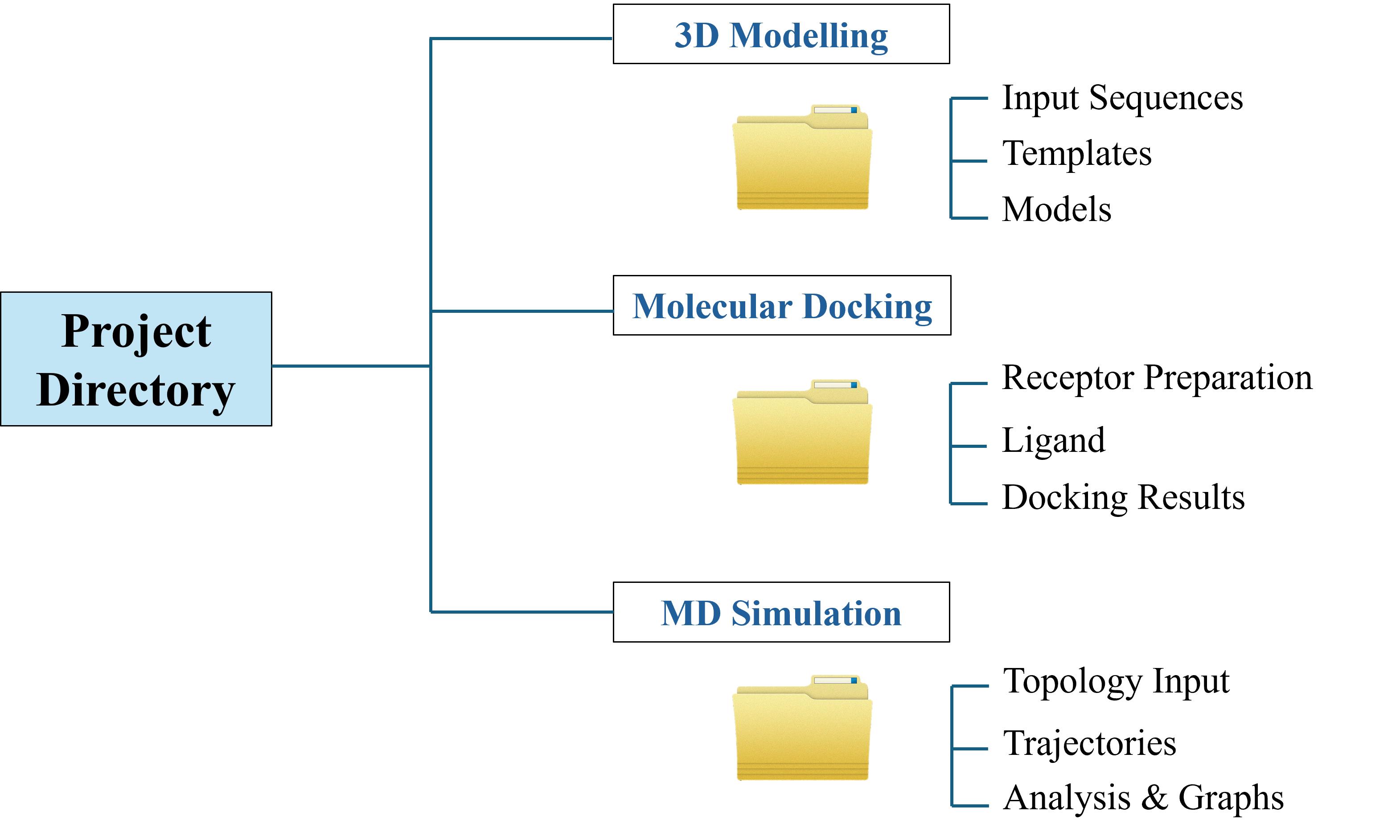
Figure 1. Directory structure for the in silico workflow
Procedure
Critical: Before initiating the procedure, it is essential to clearly define the underlying biological questions the study aims to address. This step guides the selection of ligands, protein targets, docking strategies, and simulation parameters. It is also important to note that specific settings such as force fields, simulation durations, and docking protocols should be tailored to the study’s objectives. This protocol focuses on investigating the interaction between mitragynine, the primary alkaloid from Mitragyna speciosa, and the GABA (A) receptor, specifically at the α/γ interface of the α5β2γ2 subtype.
A. Data preparation
1. Access the Protein Data Bank (PDB): Visit the PDB website at https://www.rcsb.org/.
2. Search for the target protein: Enter the name of the selected protein target [e.g., human GABA(A) receptor] into the search bar. To refine the results, apply filters such as release date (e.g., 2020–2025).
3. Select the appropriate PDB entry: Identify and download the specific structure needed for the study. For this protocol, the structure with PDB ID 8SGO is used (see Figure 2).
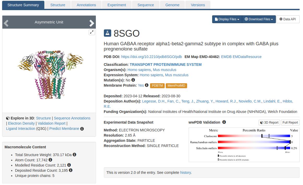
Figure 2. Structure summary of GABA (A) receptor, PDB ID: 8SGO
4. Download the structure file: Download the selected protein structure in .pdb format from the PDB entry page.
5. Check for missing residues: Open the PDB file using a text editor and use the search function (Ctrl+F) to identify any missing residues in the sequence. These are typically indicated by remarks or discontinuities in residue numbering (see Figure 3).
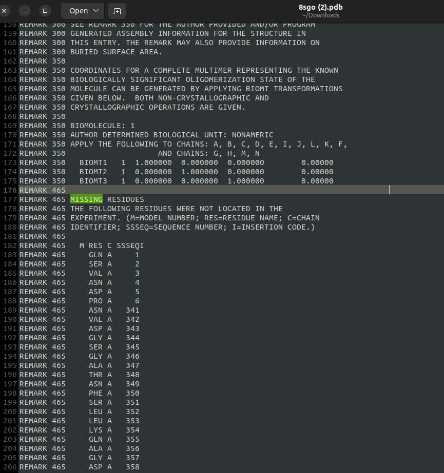
Figure 3. Missing residues of the GABA (A) receptor
6. Load the structure into PyMOL: Open the downloaded PDB file in PyMOL to visualize and edit the 3D protein structure.
7. Display the protein sequence: Click the S (Sequence) button at the bottom right of the PyMOL interface to display the amino acid sequence above the 3D structure.
8. Color-code by chain: Click the C (Colour) → by chain button in the top-right corner of the PyMOL to assign a unique color to each protein chain for easier visualization.
9. Identify non-protein molecules: In the sequence display, click on non-protein components (e.g., ligands such as NAG, BMA, Q3G, PTY, A8W, ABU) to select them (see Figure 4).
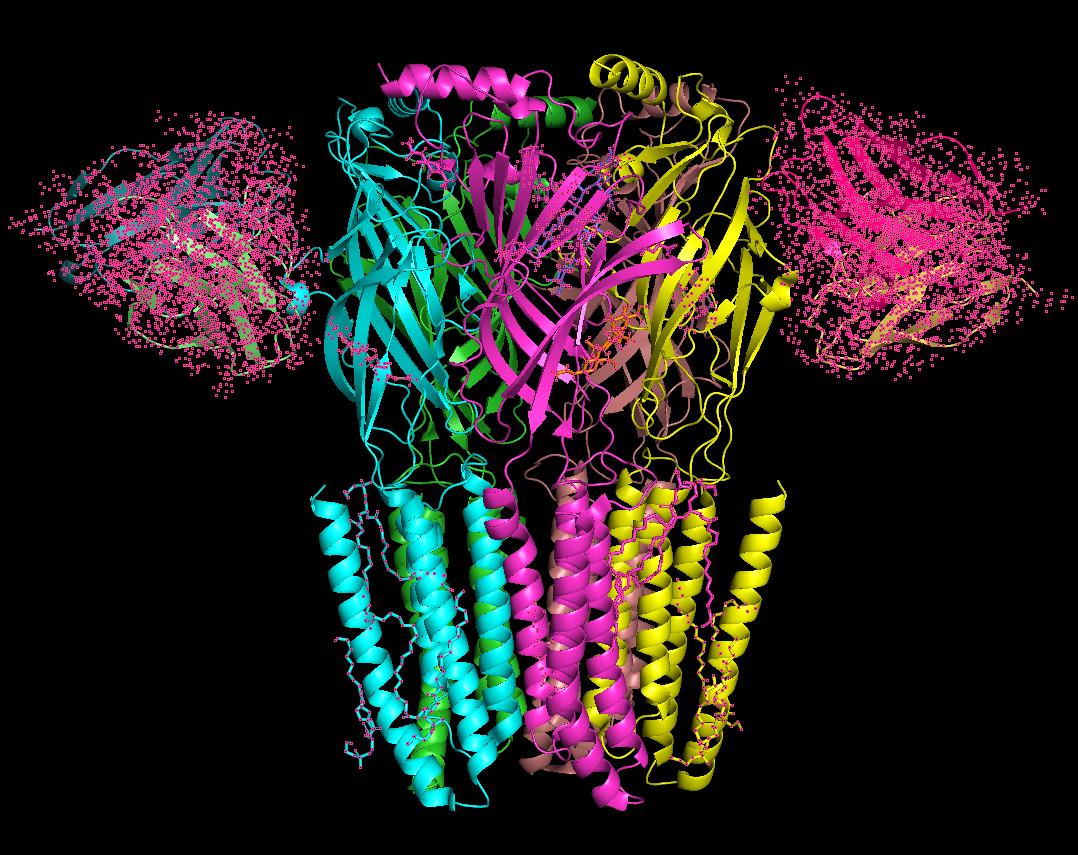
Figure 4. 3D structure of the GABA (A) receptor with unwanted molecules (pink dot)
10. Remove selected atoms: Click the A (Action) button next to [sele], then choose remove atoms to delete the selected non-protein components.
11. Export the cleaned structure: Go to File → Export Molecule, and save the cleaned structure in .pdb format, replacing the original file if desired. The protein is now ready for further analysis.
B. Molecular modeling in pharmaceutical research
In pharmaceutical research, molecular modeling plays a pivotal role in drug discovery and development. By simulating interactions between potential drug candidates and biological targets such as proteins or nucleic acids, researchers can identify promising compounds more efficiently and cost-effectively. Molecular modeling allows us to visualize molecular interactions at the atomic level, imagine zooming into a microscopic world where individual atoms interact in real time. This capability enables structural predictions, interaction assessments, and informed drug design decisions. One key application is predicting the 3D structure of proteins from their amino acid sequences [22]. These predicted structures, or those derived from experimental data, form the foundation for downstream analyses such as docking and molecular dynamics simulations. Structural data can be retrieved from the Protein Data Bank (PDB), which houses experimentally determined protein structures obtained via techniques like cryo-electron microscopy (cryo-EM) and X-ray crystallography [23].
Software installation: MODELLER
To perform 3D modeling of protein structures, MODELLER must be installed. Visit the official site at https://salilab.org/modeller/download_installation.html and download the appropriate installer for your operating system. Follow the installation guide provided on the MODELLER website.
B1. Template selection for GABA (A) receptor modeling
Molecular modeling of the GABA (A) receptor involves constructing a 3D model based on an available crystal structure, a process known as comparative (or homology) modeling. This technique begins with aligning the amino acid sequence of the target protein to a known template structure. In the absence of a high-resolution experimental structure for the desired subtype, a closely related template can be used. This approach provides flexibility in building receptor models with specific subunit compositions. In this protocol, the α1β2γ2 subtype (PDB ID: 8SGO) was selected as the template for modeling the α5β2γ2 subtype. The specific subunit composition required for modeling is summarized in Table 4.
Table 4. Chain identification in the reference template and constructed model
| Chain | Template (PDB ID: 8SGO) | Model (α5β2γ2) |
| A | β2 | β2 |
| B | α1 | α5 |
| C | β2 | β2 |
| D | α1 | α5 |
| E | γ2 | γ2 |
B2. Full-length subunit retrieval
1. Retrieve UniProt and AlphaFold entries: For each required subunit, obtain the corresponding UniProt ID from https://www.uniprot.org and the AlphaFold ID from https://alphafold.ebi.ac.uk.
2. Download the 3D structure of each subunit: Click on the accession number (see Figure 5) to access the structure page, then download the file in PDB format. Rename each file to correspond with its respective subunit for clarity and systematic organization.
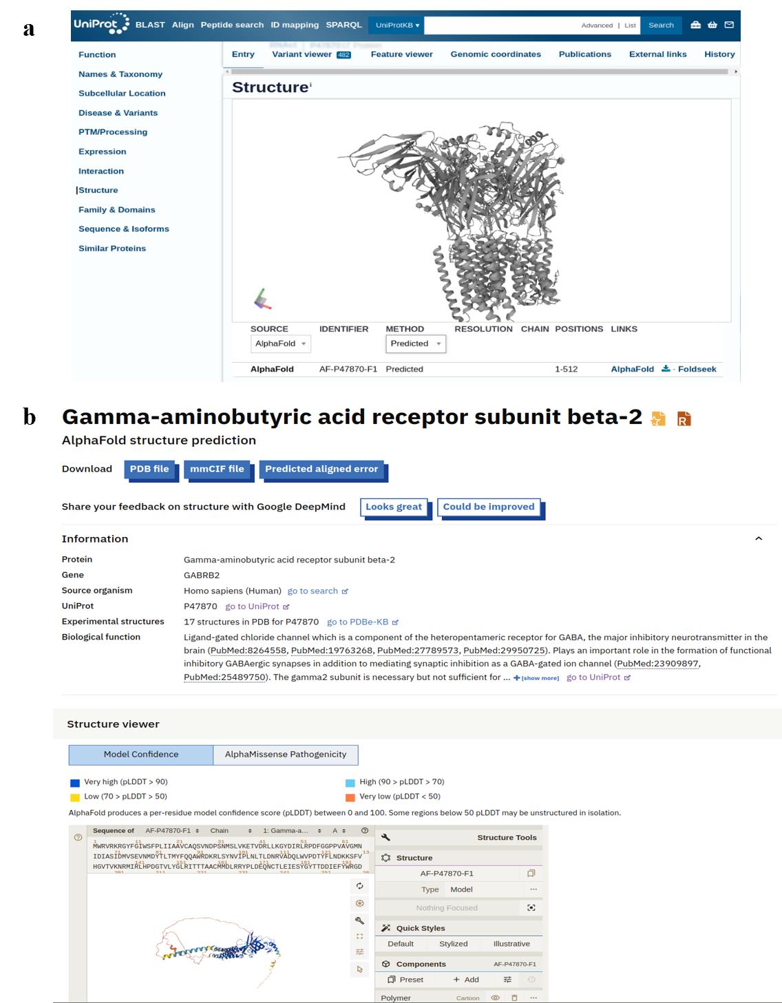
Figure 5. Structure summary of the GABA (A) receptor for each subunit from (a) UniProt and (b) AlphaFold database
B3. Sequence alignment
1. Open PyMOL: Launch PyMOL and load the 3D structures of the individual subunits.
2. Load the template structure: Import the template structure (PDB ID: 8SGO) into PyMOL. Align each subunit of the model with the corresponding subunit in the template, as indicated in Table 5 and shown in Figure 6. Use the following command:
align a5, 8sgoTable 5. Chain and subunit identification in template and model structures
| Chain/color | Subunit | Template/model |
| A (green) | β2 | Template |
| B (blue) | α1 | Template |
| C (magenta) | β2 | Template |
| D (yellow) | α1 | Template |
| E (pink) | γ2 | Template |
| D’ (red) | α5 | Model |
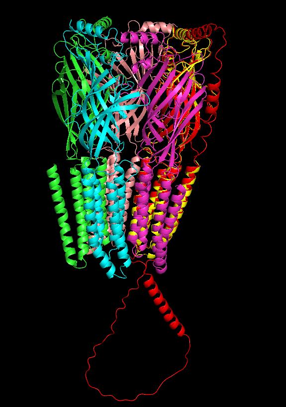
Figure 6. Superimpose the position of the α5 subunit with chain D using PyMOL
3. Export aligned subunits individually: Click on the aligned model subunit (e.g., α5, displayed in red), then export the selected molecule ([sele]) as a PDB file. Rename the file based on its corresponding chain ID. Repeat this step for each subunit, as shown in Figure 7, by selecting the appropriate chain. To align β2 with chain A, click on chain A in PyMOL and use the following command:
align β2, sele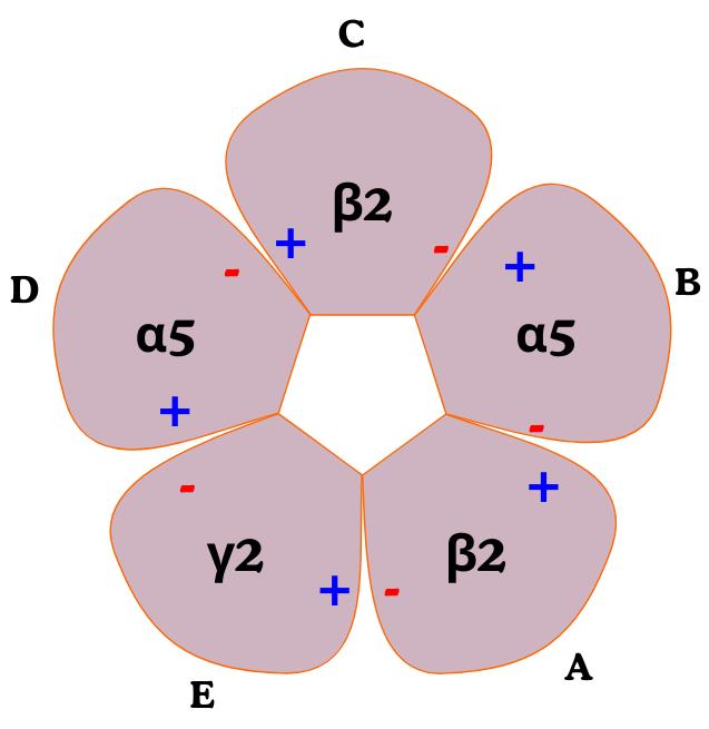
Figure 7. Arrangement of the GABA (A) receptor α5β2γ2 subtype
4. Extract full-length sequences using MODELLER: To obtain the full-length sequence for each chain, use MODELLER to import the structure and extract the sequence. Create a Python script named getsequence.py to generate the sequence file. Make sure to reference the template structure using the PDB ID 8SGO in the script and save the file accordingly (see Figure 8).
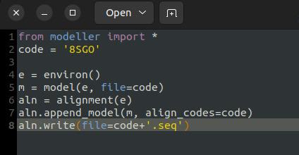
Figure 8. getsequence.py script of MODELLER
5. Run MODELLER to extract the amino acid sequence: Open a terminal and execute MODELLER (version 10.7 or the version installed on your system) to run the script and obtain the amino acid sequence with the following command:
mod10.7 getsequence.py6. Modify the script for each chain: Before running the script each time, update the code to specify the identifier for the chain (e.g., A, B, C, D, E); then, save the changes.
7. Prepare sequences for alignment: Copy the output sequence obtained from MODELLER and align it with the model sequence. Open a text editor and paste both sequences, one from the PDB file and the other from AlphaFold, in corresponding order.
8. Perform multiple sequence alignment (MSA): Go to the EBI Clustal Omega web server at https://www.ebi.ac.uk/jdispatcher/msa/clustalo and conduct an MSA for each chain’s sequences. Set the output format to PHYLIP and select protein as the sequence type (see Figure 9). Save each alignment file with the corresponding chain identifier, e.g., A.phylip. Repeat this process for chains B, C, D, and E.
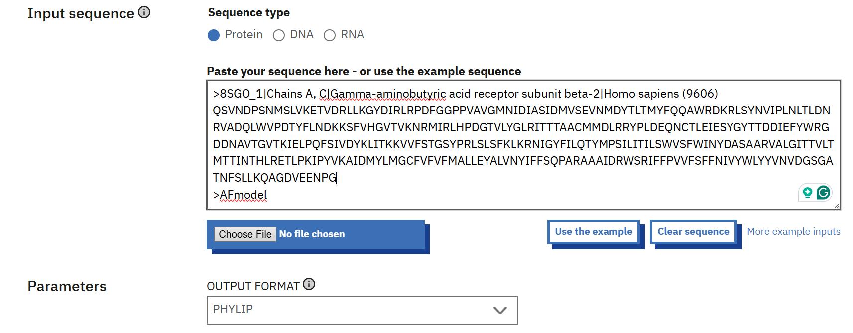
Figure 9. Multiple sequence alignment of template and model for each chain using Clustal Omega
9. Convert PHYLIP files to PIR format: Download the output files from Clustal Omega and upload them to the online sequence conversion tool at https://sequenceconversion.bugaco.com/converter/biology/sequences/pir_to_phylip.php. Convert each PHYLIP file to PIR format by selecting the protein option. Save the converted files with the corresponding chain identifier, for example, A.pir. Repeat this process for the other chains (B, C, D, and E) (see Figure 10).
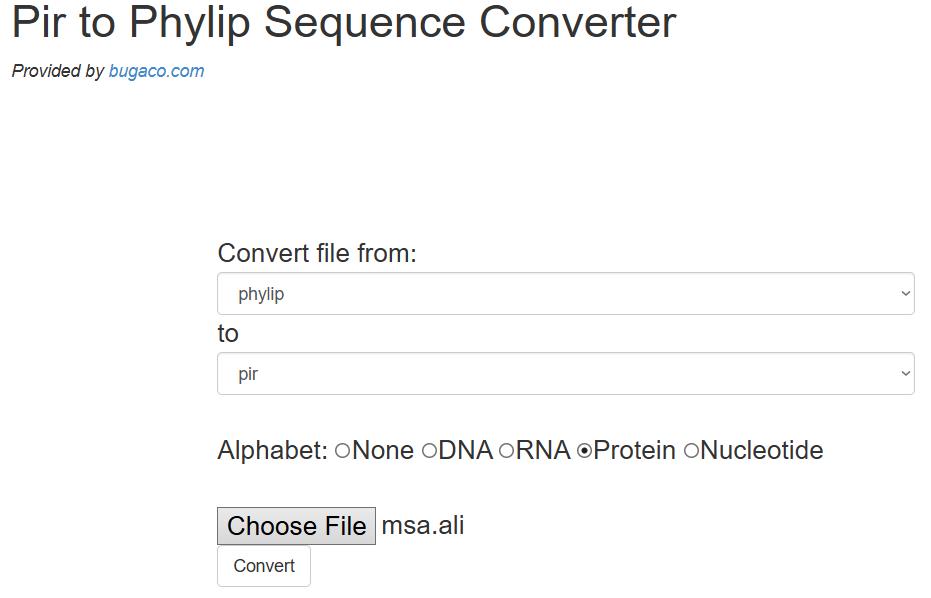
Figure 10. Online converter of PHYLIP to PIR format
10. Prepare sequences for alignment: Copy the sequence from the PDB file to serve as the template, and the sequence from AlphaFold as the model.
11. Assign chain identifiers: For each chain of the GABA (A) receptor (chains A, B, C, D, and E), insert the corresponding identifier obtained from getsequence.py by updating the code for each chain individually.
12. Edit the alignment file: Open the 8sgo.seq file and copy the chain identifiers into your alignment text editor. Populate the text editor with the complete sequences for each chain. Then, arrange the alignment as follows: first, include the 8SGO template sequence, followed by the full sequence for each chain, and lastly, the full-length model sequence. For sequence alignment, insert gaps (-) as needed to ensure proper alignment of sequences and numbering. Save the final multiple sequence alignment file as msa.ali (see Figure 11).
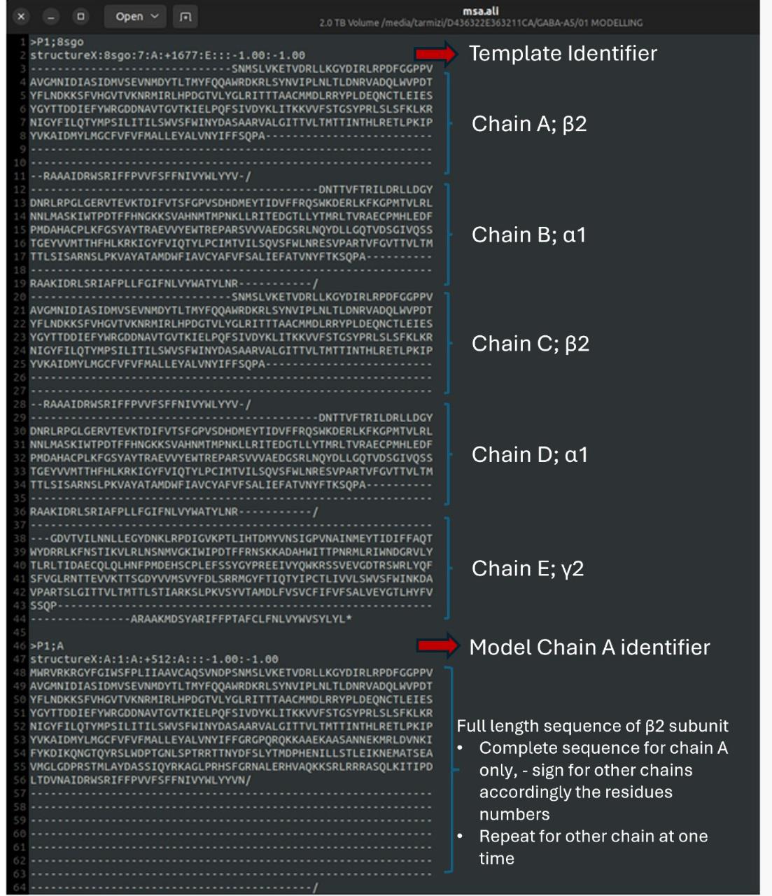
Figure 11. Multiple sequence alignment between the template and model of α5β2γ2
B4. Homology modeling
1. Create the modeling script: Using MODELLER, create a script named model_evaluate.py to construct the homology model (see Figure 12). Ensure that the file names in the script correctly correspond to the sequence files and known template structures.
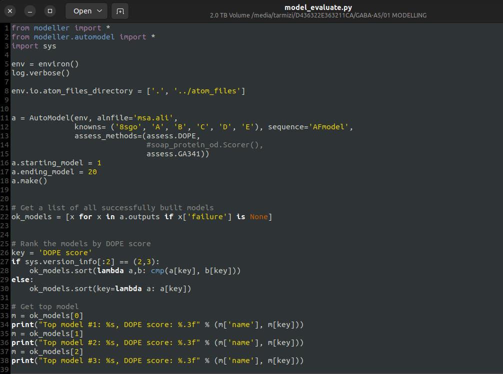
Figure 12. Python file for model evaluation using MODELLER 10.7
2. Run the modeling script: Open a terminal and execute MODELLER using the following command: mod10.7 model_evaluate.py. This will generate 20 output 3D protein models ranked based on their DOPE scores. Open the model_evaluate.log file to review the list of generated models and their scores.
3. Select and visualize the best model: Among 20 generated models, select the structure exhibiting the lowest DOPE score, along with favorable stereochemical quality from Ramachandran plot (>90% residues in allowed regions) and high ERRAT score, reflecting good overall model reliability. Choose the best 3D structure, rename it as completemodel.pdb, and visualize it using PyMOL. Load the original protein structure (prior to modeling) and superimpose the two models to compare their conformations. Use the command: align completemodel, 8sgo (Figure 13).
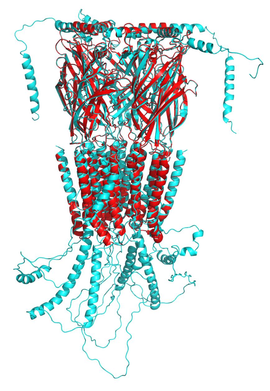
Figure 13. Comparison between the template (red cartoon representation) and model (cyan cartoon representation) with a root mean square deviation (RMSD) value of 0.332
4. Assess model quality: Evaluate the quality of the homology model to ensure its reliability for subsequent molecular docking.
5. Structure validation and refinement: Upload the completed PDB structure to the UCLA-DOE LAB server and assess it using ERRAT and PROCHECK tools.
6. If the model yields a low ERRAT score, perform structure refinement using GROMACS and CHARMM-GUI software before proceeding.
B5. Refinement using CHARMM-GUI and GROMACS
B5.1. Preparation of input files
1. Open the CHARMM-GUI website (https://www.charmm-gui.org/) and create a free account using a non-commercial email address. Log in to access CHARMM-GUI.
2. Since the GABA (A) receptor is a membrane protein, navigate to Input Generator and select Membrane Builder → Bilayer Builder (see Figure 14).
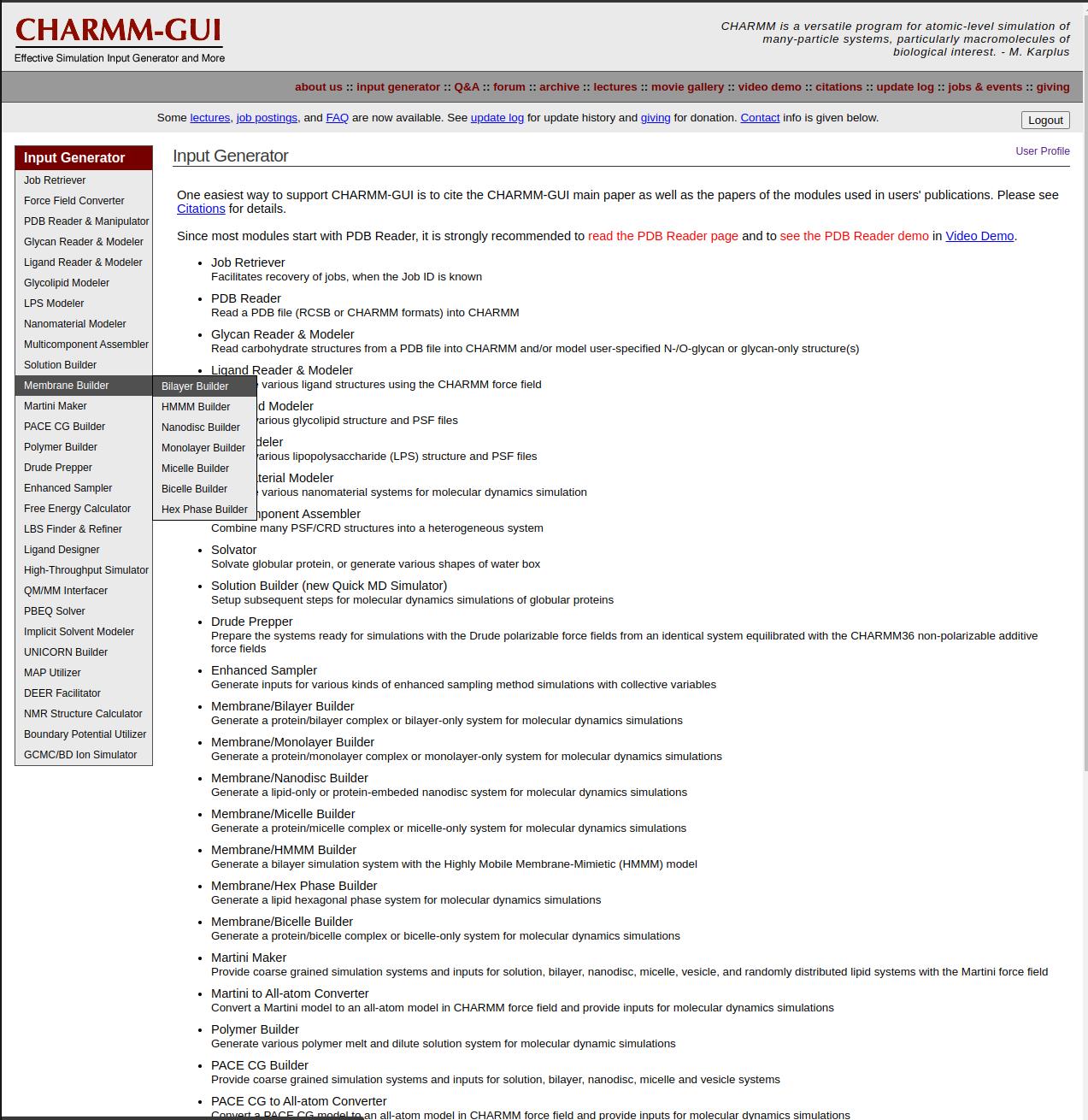
Figure 14. CHARMM-GUI Input Generator interface, highlighting the available modules for system setup for bilayer model membrane
3. Upload and prepare the protein structure:
a. Select Protein/Membrane system and upload the 8sgo.pdb file.
b. Ensure the box for PDB format is checked.
c. Verify and correct the PDB format, if necessary, before proceeding.
4. Select chains: Choose the protein chains to include in the system, then proceed to the next step.
5. Orient the protein in the membrane: After processing, select Run PPM 2.0 to orient the protein within the lipid bilayer system.
6. Set system size: Scroll to System Size Determination Options and:
a. Select Heterogeneous Lipid option.
b. Specify the box type as Rectangular.
c. Set the Z dimension length based on water thickness (22.5 Å).
d. Set the XY dimensions based on the number of lipid components.
7. Specify lipid composition: Further down, in the Lipid Information section:
a. Choose PC (phosphatidylcholine) Lipids, select POPC.
b. Adjust the lipid ratios for the upper and lower leaflets as needed before proceeding.
8. System building options:
a. Select Replacement Method and check Check Lipid Ring (and Protein Surface) Penetration.
b. Under Component Building Options, keep the default system settings.
c. For Include Ions, select Ion placing method based on distance, with Basic Ion Types set to KCl at 0.15 M. Add NaCl Simple Ion Type to the system.
d. Click Calculate Solvent Composition.
e. Click Next to start the lipid packing process.
9. Force field and input generation:
a. From the Force Field Options dropdown, select CHARMM36m.
b. Under Input Generation Options, unclick the More CHARMM minimization during input generation box, then choose GROMACS.
c. Check the boxes to Generate grid information for PME FFT automatically.
d. Select NPT ensemble at Temperature: 310.15 K.
e. Proceed to the next step to generate equilibration and dynamics input files.
10. Download input files: Carefully read the Equilibration Input Notes and download all input files to your working folder.
B5.2. Energy minimization using GROMACS
1. Navigate to your working directory and open the charmm-gui/gromacs folder, which contains the input files for the GROMACS simulation.
2. Open the README file for guidance on the command lines. On line 26, replace gmx_d with gmx and save the file.
3. Start the energy minimization process by running the following commands in the terminal:
gmx grompp -f step6.0_minimization.mdp -o step6.0_minimization.tpr -c step5_input.gro -r step5_input.gro -p topol.top -n index.ndxgmx mdrun -v -deffnm step6.0_minimizationB5.3. System equilibration using GROMACS
1. Perform the 5-step NVT equilibration by running the following commands sequentially:
NVT equilibration for 125 ps
gmx grompp -f step6.1_equilibration.mdp -o step6.1_equilibration.tpr -c step6.0_minimization.gro -r step5_input.gro -p topol.top -n index.ndxgmx mdrun -v -deffnm step6.1_equilibrationNVT equilibration for 125 ps
gmx grompp -f step6.2_equilibration.mdp -o step6.2_equilibration.tpr -c step6.1_equilibration.gro -r step5_input.gro -p topol.top -n index.ndxgmx mdrun -v -deffnm step6.2_equilibrationNVT equilibration for 125 ps
gmx grompp -f step6.3_equilibration.mdp -o step6.3_equilibration.tpr -c step6.2_equilibration.gro -r step5_input.gro -p topol.top -n index.ndxgmx mdrun -v -deffnm step6.3_equilibrationNVT equilibration for 500 ps
gmx grompp -f step6.4_equilibration.mdp -o step6.4_equilibration.tpr -c step6.3_equilibration.gro -r step5_input.gro -p topol.top -n index.ndxgmx mdrun -v -deffnm step6.4_equilibrationNVT equilibration for 500 ps
gmx grompp -f step6.5_equilibration.mdp -o step6.5_equilibration.tpr -c step6.4_equilibration.gro -r step5_input.gro -p topol.top -n index.ndxgmx mdrun -v -deffnm step6.5_equilibration2. Perform NPT equilibration for 500 ps with the following commands:
gmx grompp -f step6.6_equilibration.mdp -o step6.6_equilibration.tpr -c step6.5_equilibration.gro -r step5_input.gro -p topol.top -n index.ndxgmx mdrun -v -deffnm step6.6_equilibration3. Extract protein structure from trajectory file. To extract the protein receptor structure from the simulation trajectory, use the command:
gmx trjconv -f step7_production.xtc -s step7_production.tpr -o structure.pdb -dump 500C. Molecular docking
In recent years, molecular docking has become a key component of in silico drug development, enabling detailed predictions of how compounds interact with target proteins. This approach allows researchers to examine the binding behavior of small molecules, such as nutraceuticals, within the active sites of target proteins and to gain insights into the molecular basis of these interactions [24]. For specific targets, scoring functions can be applied to evaluate a ligand’s binding conformation and position within the binding site, estimate its binding affinity, and support the identification of promising therapeutic candidates [25].
C1. Preparation of ligands
1. Create a dedicated folder for docking, which should contain the PDB structures of both the protein target (from homology modeling) and the ligands.
2. Visit the PubChem website.
3. Search for mitragynine using the search bar.
4. Download the 3D structure of mitragynine in SDF format and save it in the designated docking folder.
5. Convert the SDF file to PDB format using PyMOL:a. Open the SDF file in PyMOL.
b. Navigate to File → Export Molecule, ensure the molecule is selected, and save the file as PDB.
C2. Molecular docking using AutoDock Tools (ADT) and AutoDock Vina
1. Launch AutoDock Tools (ADT) and load the protein structure: Go to File → Read Molecule and select the file (e.g., 8SGO.pdb).
2. Prepare the protein by optimizing its structure:
a. Add hydrogens: Edit → Hydrogen → Add → Polar Only → OK
b. Compute charges:
i. Edit → Charges → Add Kollman Charges
ii. Edit → Charges → Compute Gasteiger
iii. Edit → Charges → Check Totals on Residues → Dismiss
3. Define the macromolecule for docking:
Grid → Macromolecules → Choose → Select 8SGO → OK
4. Save the prepared protein structure in PDBQT format in the docking directory.
5. Load the ligand (mitragynine):
File → Read Molecule → Select the mitragynine PDB file → OK
6. Save the ligand structure in PDBQT format:
Go to Ligand → Output → Save as PDBQT
7. Define the docking site:
a. Grid → Grid Box
b. Highlight and include key amino acid residues if necessary.
c. Set the grid box to cover the extracellular domain of the GABA (A) receptor at the predicted ligand binding site. Adjust its center and dimensions using wheels on Center Grid Box.
d. Example grid box parameters: For docking at the α/γ interface, which corresponds to the benzodiazepine (BZD) binding pocket, the grid box was positioned at coordinates (center_x = 79.676, center_y = 99.096, center_z = 62.909) and defined with dimensions of (size_x = 36 Å, size_y = 36 Å, size_z = 40 Å).
8. Set the grid spacing to 1.0 Å instead of 0.375 Å, following the optimal grid spacing docking algorithm.
9. Save the docking configuration as a conf.txt file using a text editor and save it in the docking directory (see Figure 15 for reference).
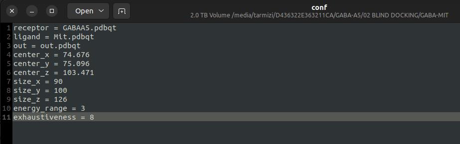
Figure 15. Configuration of the grid box
10. Open a terminal window in the docking directory and run the docking simulation using the command below. Be sure to record the output data for analysis (see Figure 16 for reference). Use the following command:
vina --config conf.txt --log log.txt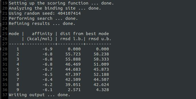
Figure 16. Value of docking energy
11. To separate the docking output poses into individual files, use the following command in the terminal:
vina_split --input out.pdbqtC3. Analysis of interactions (AutoDock Tools)
1. In AutoDock Tools (ADT), navigate to:
a. Analyze → Docking → Open AutoDock Vina Results → Select out_ligand_1 → Choose Single molecule with multiple conformations → Click OK.
b. Change the representation to L (lines) and B (ball and stick).
Note: The selected out_ligand file should represent the ligand pose with the best orientation and conformation at the extracellular binding interface of the GABA (A) receptor.
2. Load the macromolecule: Analyze → Macromolecule → Open → Select 8SGO → Change its representation to R (ribbon).
3. Visualize interactions: Analyze → Docking → Show Interactions.
4. Export the ligand: Select (S) out_ligand_5 → File → Save → Write PDB → Save in docking directory as ligand.pdb.
5. Export the receptor-ligand complex:
a. Deselect out_ligand_5.
b. Select (S) 8SGO → File → Save → Write PDB → Save as receptor_ligand.pdb.
6. Open ligand.pdb in a text editor and copy the contents starting from the second line.
7. Open receptor_ligand.pdb in the same text editor, scroll to the bottom, paste the copied ligand content after the last line, and save the file.
C4. Visualization and analysis in PyMOL
1. Open receptor_ligand.pdb in PyMOL.
2. Display the sequence: Click S at the bottom right to show the sequence viewer.
3. Scroll to the end of the sequence and select the ligand.
4. On the ligand selection (sele): Click Action (A) → find → polar contacts → to others excluding solvent.
5. Run the following command to select nearby residues:
select close, br. polymer near_to 5 of (sele)6. In the object list selection (close): Change the 3D representation by clicking Show → sticks.
7. Left-click the ligand and all interacting residues (indicated by yellow dashed lines).
8. Hide unselected elements: Go to (sele) → Hide (H) → unselected.
9. Apply color to the ligand and interacting residues according to your preferred scheme.
10. Label residues: Left-click each interacting amino acid → Label → residues.
11. Measure hydrogen bond distances: Click Wizard → Measurement → Select two points between the ligand and each interacting residue → Click Done to exit.
12. Save a high-quality image: Click Draw/Ray at the top-right → Set DPI to 300 → Click Ray (slow) → Save the image.
C5. Binding interaction analysis programs
Protein–Ligand Interaction Profiler (PLIP)
1. Upload the receptor_ligand.pdb file to the PLIP web server.
2. Click Analyze to generate interaction results.
3. Review the list of detected interactions (e.g., hydrogen bonds, hydrophobic contacts, salt bridges).
4. Download the interaction output files.
5. Open the visualized interaction files in PyMOL for further inspection and figure generation.
BIOVIA Discovery Studio 2021
1. Launch BIOVIA Discovery Studio 2021.
2. Navigate to File → Open and select the receptor_ligand.pdb file.
3. Go to Tools → Binding Analysis → Ligand Interactions.
4. Click Show Interactions to visualize key contacts such as hydrogen bonds, hydrophobic interactions, pi-stacking, and salt bridges.
Note: Repeat the docking and interaction analysis steps for each ligand of interest. Rename the output files or complexes accordingly for systematic organization and clarity.
C6. Superimposition with GABA neurotransmitter
1. Open the docked complex in PyMOL [e.g., GABA (A)R–Mitragynine complex].
Note: GABA is the native neurotransmitter for GABA (A) receptors. In the α5β2γ2 subtype, GABA typically binds at the β+/α− interface, while compounds like mitragynine are proposed to bind at the α+/γ− interface. Superimposing the docked complex with a GABA-bound structure helps highlight site specificity.
2. Superimpose the docked complex with the original template used during homology modeling (PDB ID: 8SGO).
3. In the PyMOL command line, execute Fetch 8SGO and press ENTER. 2nd command: Align 8SGO, GABA-MIT (depends on the actual file name).
4. Remove unwanted components from the template structure: Delete irrelevant ligands and heavy/light chains, retaining only the GABA molecule (e.g., ABU) and the docked protein–ligand complex.
5. Export the final superimposed complex (with both GABA and mitragynine) to PDB format for visualization or figure generation (see Figure 17 for reference).
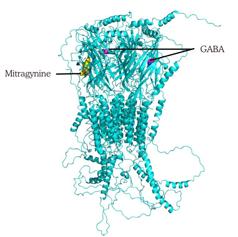
Figure 17. Superimposition of α5β2γ2–mitragynine complex with GABA bound
D. Molecular dynamics simulation
Molecular dynamics (MD) simulation models a system at the atomistic level by representing solute and solvent as a collection of interacting particles, each corresponding to individual atoms. These particles are placed within a sufficiently large simulation box, allowing the system to capture their dynamic trajectories. Their motion follows Newton’s classical laws of motion, specifically Newton’s second law F = ma, where the force F acting on each particle determines its acceleration a based on its mass m under a potential field [26,27]. Interatomic forces are calculated using potential models such as Lennard-Jones for van der Waals interactions and Coulomb’s law for electrostatics, which together govern the key atomic interactions driving the system’s behavior [28]. MD simulations serve as molecular microscopes that enable detailed evaluation of ligand stability within receptor binding pockets, providing a way to validate molecular docking predictions.
In this study, MD simulations are performed using the Groningen Machine for Chemical Simulations (GROMACS) software. The receptor–ligand complexes are embedded in a lipid bilayer constructed with the CHARMM-GUI bilayer builder [29]. Each complex is inserted into a POPC bilayer and solvated with TIP3P water molecules following proper PDB processing and orientation. The system components, including lipids, water molecules, ions, and simulation box dimensions, are configured accordingly. Output files from CHARMM-GUI are then used for energy minimization and system equilibration, a crucial step that alleviates geometric and structural clashes caused by residue movements, allowing the system to relax toward its global minimum energy state.
D1. Ligand preparation using CHARMM-GUI Ligand Reader & Modeler
1. Upload the ligand structure file (ligand.pdb) obtained from molecular docking to the Ligand Reader and Modeler module in CHARMM-GUI. Click on Upload PDB/CIF, then select the LIG undefined option (see Figure 18).
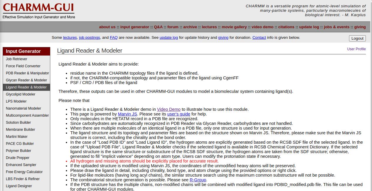
Figure 18. Ligand Reader & Modeler of CHARMM-GUI
2. Verify that the 2D structure of the ligand is correctly displayed before proceeding to the next step (see Figure 19).
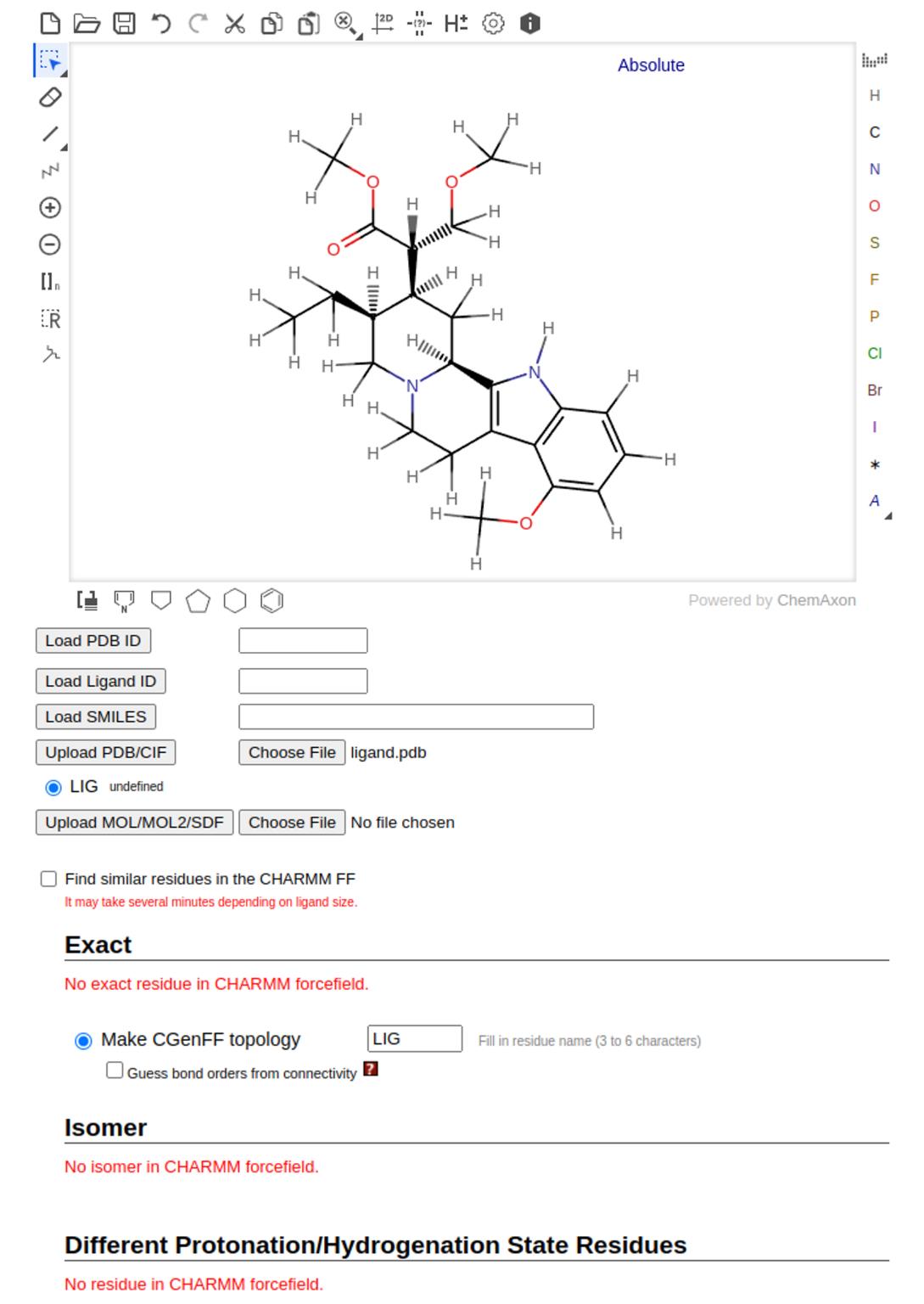
Figure 19. 2D structure of mitragynine as ligand defined using CHARMM-GUI
3. Confirm that the ligand name (LIG) matches the uploaded ligand file name. Then, click Next to generate the PDB file.
4. In the same folder as the MD simulation files, download the following output files: the topology file (lig.rtf), the parameter file (lig.prm), and the updated ligand structure (ligandrm.pdb) (see Figure 20).
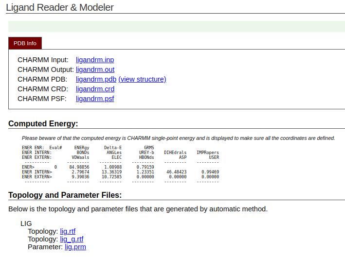
Figure 20. Parameter and topology files of the ligand from CHARMM-GUI
5. Integrate the new ligand structure into the protein complex. Open ligandrm.pdb in a text editor, copy all lines starting from the second line, and paste these atomic coordinates into the receptor_ligand.pdb file (the combined complex structure).
6. Navigate to Membrane Builder → Bilayer Builder in CHARMM-GUI. Upload the new receptor_ligand.pdb file and click Next to proceed.
7. On the PDB manipulation page, select Hetero (HETA) to retain the ligand during system preparation. Then, click Next to continue (see Figure 21).
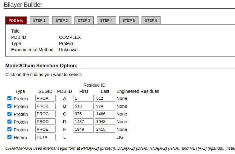
Figure 21. Chain selection of the protein and ligand (hetero) from CHARMM-GUI
8. Choose the option to upload CHARMM topology and parameter files for the hetero chain. Upload the lig.rtf and lig.prm files into the appropriate sections (see Figure 22). Click Next to generate the PDB file and orient the molecule. The ligand is now correctly recognized by CHARMM-GUI, and the system is ready for the generation of input files for molecular dynamics simulation.
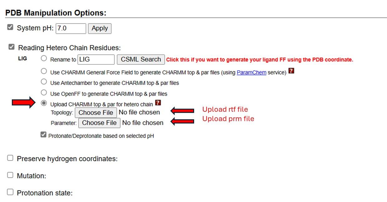
Figure 22. PDB manipulation options of topology and parameter files
D2. Preparation of input files, energy minimization, and system equilibration
1. Follow Part B: Molecular Modeling (step B5) to generate output files for simulation.
2. Perform the energy minimization and system equilibration (NVT and NPT only, without extracting the trajectory file) using GROMACS.
D3. MD production using GROMACS
1. Open the step7_production.mdp file in a text editor and add the following line to enable trajectory output:
nstxtcout = 50000
This setting specifies the frequency of writing coordinates to the .xtc trajectory file (see Figure 23). Save the file before proceeding.
Note: Change the nsteps according to the required simulation time, e.g., for 100 ns. Generally, the recommended minimum duration for membrane or receptor–ligand systems to achieve structural equilibrium and reliable sampling of dynamics conformations is 100 ns [30].
1 ns = 1000 ps
100 ns = 100000 ps.
Nsteps = 100000/0.002 → dt
= 50000000 steps

Figure 23. MDP file for MD production
2. Start the molecular dynamics (MD) production run by executing the following command in the terminal:
gmx grompp -f step7_production.mdp -o step7_production.tpr -c step6.6_equilibration.gro -p topol.top -n index.ndxgmx mdrun -v -deffnm step7_productionThis command will launch the production phase of the simulation using the parameters defined in the modified .mdp file.
Note: If the simulation is interrupted or stops unexpectedly, it can be resumed by extending the run using the checkpoint file (.cpt). Use the following command to continue the simulation:
gmx mdrun -v -deffnm step7_production -cpi step7_production_prev.cptThis command continues the production run from the last saved state stored in the checkpoint file.
D4. Data analysis
The stability of MD simulation is commonly evaluated through several key parameters, including root mean square fluctuation (RMSF), radius of gyration (Rg), root mean square deviation (RMSD), and hydrogen bond occupancy. These metrics reflect the equilibrium state and structural consistency of the protein–ligand complex during simulation. Table 6 presents the typical stability ranges observed in well-equilibrated receptor–ligand systems, serving as a reference for interpreting the results.
Table 6. Benchmark stability metrics commonly used to evaluate convergence and structural consistency during protein–ligand MD simulations
| Parameter | Description | Expected stable range | References |
| RMSD (Å) | Deviation of protein backbone over time | <5.0 | [31] |
| RMSF (Å) | Residue-level flexibility | 0.5–3.0 | [32] |
| Radius of gyration (Å) | Compactness of protein structure | ~22 (depending on protein size) | [33] |
| Hydrogen bonds | Number of protein–ligand hydrogen bonds | 2–5 (persistent) | [34] |
1. Begin by analyzing the trajectory file generated during the simulation. Convert step7_production.trr into a centered and more manageable .xtc file (step7_production_center.xtc) for use in subsequent analysis steps. Use the following command:
gmx trjconv -s step7_production.tpr -f step7_production.trr -o step7_production_center.xtc -pbc cluster -centerSelect group 1 (“Protein”) when prompted for the clustering group and press Enter.
Next, select group 1 (“Protein”) again to specify the group for centering and press Enter. Finally, select group 0 (“System”) for the output and press Enter.
2. Calculate the temperature fluctuations and total energy of the system.
gmx energy -f step7_production.edr -s step7_production.tpr -o temperature.xvgSelect group 15 (“Temperature”) and press Enter, then select 0 to begin the calculation. The resulting temperature graph can be visualized using xmgrace.
xmgrace temperature.xvg3. For total energy calculation,
gmx energy -f step7_production.edr -s step7_production.tpr -o totalenergy.xvgSelect group 13 (“Total Energy”) and press Enter, then select 0 to begin the calculation. The resulting total energy graph can be visualized using xmgrace.
xmgrace totalenergy.xvg4. Root mean square deviation (RMSD) is used to quantify how much the protein structure deviates from its initial conformation over the course of the simulation. To calculate RMSD,
gmx rms -s step7_production.tpr -f step7_production_center.xtc -o rmsd.xvg -tu nsChoose group 4 (“Backbone”) twice for the least-squares fitting and the group for RMSD calculation. Visualize the RMSD results using xmgrace.
xmgrace rmsd.xvg5. The radius of gyration (Rg) is an important metric to assess whether the protein remains properly folded and maintains its compactness during the simulation. A stable Rg value indicates structural stability, while an increase suggests protein unfolding. To calculate the radius of gyration,
gmx gyrate -s step7_production.tpr -f step7_production_center.xtc -o gyrate.xvg -tu nsSelect group 1 (“Protein”) for the radius of gyration calculation. Visualize the gyration results using xmgrace.
xmgrace gyrate.xvg6. Root mean square fluctuation (RMSF) measures the average deviation of each atom or residue from its mean position during the simulation, indicating flexibility. To compute RMSF,
gmx rmsf -f step7_production_center.xtc -s step7_production.tpr -o rmsf.xvg -res -n index.ndxSelect groups 1 (“Protein”) and 13 (“LIG”) for the RMSF calculation. Visualize the RMSF results using xmgrace.
xmgrace rmsf.xvg7. Calculating hydrogen bonds between the protein and ligand is important for analyzing their potential interactions. To perform hydrogen bond analysis,
gmx hbond -f step7_production_center.xtc -s step7_production.tpr -num hbond.xvg -tu ns -n index.ndxSelect groups 1 (“Protein”) and 13 (“LIG”) for the hydrogen bond calculation. Visualize the hydrogen bond analysis results using xmgrace.
xmgrace hbond.xvg8. Calculating the distance between the protein and ligand is also crucial for understanding their interactions. To perform this calculation,
gmx pairdist -f step7_production_center.xtc -s step7_production.tpr -o dist.xvg -tu ns -n index.ndxSelect groups 1 (“Protein”) and 13 (“LIG”), then press Ctrl+D to start the calculation. Visualize the distance results using xmgrace.
xmgrace dist.xvg9. Extract the PDB structure (.pdb file) from the simulation trajectory based on the selected time frame.
gmx trjconv -f step7_production_center.xtc -s step7_production.tpr -o structure.pdb -b 100000 -e 10000010. Visualize the extracted PDB structure using PyMOL to examine protein–ligand interactions. The structure can also be submitted to tools such as Protein-Ligand Interaction Profiler (PLIP) and BIOVIA Discovery Studio for further analysis.
Validation of protocol
For the validation of the protocol presented in the original article [35], we performed multiple in silico experiments focusing on the interaction between zolpidem, a commonly used hypnotic drug, and GABA (A) receptors containing the epsilon subunit. Using the same computational pipeline comprising molecular modeling, molecular docking, and molecular dynamics simulations, we assessed the binding affinity and stability of zolpidem at the receptor interface. The optimized model demonstrated close structural agreement with the template, and its predicted binding affinity aligned well with previously reported values for ligands targeting the benzodiazepine binding site [35]. The results of our study confirmed that the protocol reliably identifies significant differences in ligand–receptor interactions, consistent with known pharmacological properties of zolpidem and the functional relevance of ε-containing GABA (A) receptor isoforms, thereby validating the approach for use in this molecular context.
General notes and troubleshooting
General notes
1. Pay attention to file extensions. File extensions indicate the type of file and determine which programs can open or process it. Using an incorrect extension may cause errors or prevent the file from opening properly.
2. Always keep track of your files. Be mindful of file names and know where your files are saved or downloaded to, so you can easily locate and manage them when needed.
3. Tips for naming files:
• Use clear and descriptive file names that reflect the content or purpose.
• Stick to letters, numbers, hyphens (-), and underscores (_).
• Avoid special characters, as they may cause issues or errors in some operating systems or software.
Troubleshooting
A. Molecular modeling
1. Template structure is unavailable or incomplete: Search for alternative templates with higher sequence identity, or use known PDB structures from closely related receptor subtypes.
2. Alignment errors between target and template: Manually refine the sequence alignment if automated tools misalign critical structural or functional regions.
3. Low-quality validation results: Improve model accuracy and stability by applying energy minimization and refinement techniques.
B. Molecular docking
1. Docking scores are unusually inconsistent: Verify the preparation of both the receptor and ligand. Ensure that the correct binding site is identified and that the grid box is accurately defined for targeted docking. Use reference ligands when available to validate the docking setup.
C. Molecular dynamics (MD) simulations
1. System crashes during energy minimization: Check for bad contacts, missing atoms, or steric clashes. Apply additional minimization steps or use constraints during the equilibration phase if needed.
2. Energy minimization fails to converge: Check solvation box size and ensure ions are added correctly. Re-minimize after adjusting constraints or force field parameters.
3. Unstable RMSD or abnormal trajectory behavior: Review simulation parameters such as temperature and pressure control. Ensure that a correct and compatible force field is applied.
4. Water box or ions not properly added: Confirm that the system is correctly solvated and neutralized using appropriate tools (e.g., GROMACS).
5. Missing ligand parameters or incompatible force field: Generate ligand topology using tools like CHARMM-GUI and ensure compatibility with the chosen force field for the protein.
6. Simulation too short to observe meaningful interaction: Extend the simulation duration (e.g., beyond 100 ns) depending on the system size and research objectives.
7. Unstable trajectories or simulation crashing mid-run: Verify that energy minimization and equilibration were completed. Reduce the time step if needed and check the configuration. Ensure there are no overlapping atoms or missing parameters in the topology files.
Acknowledgments
The authors gratefully acknowledge the financial support provided by the Universiti Sains Malaysia through the Research University Team (RUTeam) Grant Scheme (Grant Number: R502-KR-RUT001-0000000404-K134).
Authors’ contribution: Conceptualization, Ahmad Tarmizi Che Has; Investigation, Syarifah Maisarah Sayed Mohamad and Ahmad Tarmizi Che Has. Writing—Original Draft, Syarifah Maisarah Sayed Mohamad and Ahmad Tarmizi Che Has; Writing—Review & Editing, Ahmad Tarmizi Che Has, Azzmer Azzar Abdul Hamid, and Khairul Bariyyah Abd Halim; Funding acquisition, Ahmad Tarmizi Che Has; Supervision, Ahmad Tarmizi Che Has, Azzmer Azzar Abdul Hamid, and Khairul Bariyyah Abd Halim.
This protocol was used in [35].
Competing interests
The authors declare that there are no conflicts of interest or competing interests associated with this work.
References
- Smart, T. G. and Stephenson, F. A. (2019). A half century of γ-aminobutyric acid. Brain Neurosci Adv. 3: e1177/2398212819858249. https://doi.org/10.1177/2398212819858249
- Sallard, E., Letourneur, D. and Legendre, P. (2021). Electrophysiology of ionotropic GABA receptors. Cell Mol Life Sci. 78(13): 5341–5370. https://doi.org/10.1007/s00018-021-03846-2
- Jacob, T. C., Moss, S. J. and Jurd, R. (2008). GABAA receptor trafficking and its role in the dynamic modulation of neuronal inhibition. Nat Rev Neurosci. 9(5): 331–343. https://doi.org/10.1038/nrn2370
- Kasaragod, V. B., Mortensen, M., Hardwick, S. W., Wahid, A. A., Dorovykh, V., Chirgadze, D. Y., Smart, T. G. and Miller, P. S. (2022). Mechanisms of inhibition and activation of extrasynaptic αβ GABAA receptors. Nature. 602(7897): 529–533. https://doi.org/10.1038/s41586-022-04402-z
- Maric, H. M., Kasaragod, V. B., Hausrat, T. J., Kneussel, M., Tretter, V., Strømgaard, K. and Schindelin, H. (2014). Molecular basis of the alternative recruitment of GABAA versus glycine receptors through gephyrin. Nat Commun. 5(1): e1038/ncomms6767. https://doi.org/10.1038/ncomms6767
- Ghit, A., Assal, D., Al-Shami, A. S. and Hussein, D. E. E. (2021). GABAA receptors: structure, function, pharmacology, and related disorders. J Genet Eng Biotechnol. 19(1): 123. https://doi.org/10.1186/s43141-021-00224-0
- Zhu, M., Abdulzahir, A., Perkins, M. G., Chu, C. C., Krause, B. M., Casey, C., Lennertz, R., Ruhl, D., Hentschke, H., Nagarajan, R., et al. (2023). Control of contextual memory through interneuronal α5-GABAA receptors. PNAS Nexus. 2(4): e1093/pnasnexus/pgad065. https://doi.org/10.1093/pnasnexus/pgad065
- Magnin, E., Francavilla, R., Amalyan, S., Gervais, E., David, L. S., Luo, X. and Topolnik, L. (2018). Input-Specific Synaptic Location and Function of the α5 GABAAReceptor Subunit in the Mouse CA1 Hippocampal Neurons. J Neurosci. 39(5): 788–801. https://doi.org/10.1523/jneurosci.0567-18.2018
- Chen, M., Koopmans, F., Gonzalez-Lozano, M. A., Smit, A. B. and Li, K. W. (2023). Brain Region Differences in α1- and α5-Subunit-Containing GABAA Receptor Proteomes Revealed with Affinity Purification and Blue Native PAGE Proteomics. Cells. 13(1): 14. https://doi.org/10.3390/cells13010014
- Eastlack, S. C., Cornett, E. M. and Kaye, A. D. (2020). Kratom—Pharmacology, Clinical Implications, and Outlook: A Comprehensive Review. Pain Ther. 9(1): 55–69. https://doi.org/10.1007/s40122-020-00151-x
- Hossain, R., Sultana, A., Nuinoon, M., Noonong, K., Tangpong, J., Hossain, K. H. and Rahman, M. A. (2023). A Critical Review of the Neuropharmacological Effects of Kratom: An Insight from the Functional Array of Identified Natural Compounds. Molecules. 28(21): 7372. https://doi.org/10.3390/molecules28217372
- Hartley, C., Bulloch, M. and Penzak, S. R. (2022). Clinical Pharmacology of the Dietary Supplement Kratom (Mitragyna speciosa). J Clin Pharmacol. 62(5): 577–593. https://doi.org/10.1002/jcph.2001
- Sanderson, M. and Rowe, A. (2019). Kratom. CMAJ. 191(40): E1105–E1105. https://doi.org/10.1503/cmaj.190470
- Schrödinger, L. and DeLano, W. (2020). PyMOL. http://www.pymol.org/pymol
- Webb, B. and Sali, A. (2016). Comparative Protein Structure Modeling Using MODELLER. Curr Protoc Bioinformatics. 54(1): e3. https://doi.org/10.1002/cpbi.3
- Abraham, M. J., Murtola, T., Schulz, R., Páll, S., Smith, J. C., Hess, B. and Lindahl, E. (2015). GROMACS: High performance molecular simulations through multi-level parallelism from laptops to supercomputers. SoftwareX.: 19–25. https://doi.org/10.1016/j.softx.2015.06.001
- Morris, G. M., Huey, R., Lindstrom, W., Sanner, M. F., Belew, R. K., Goodsell, D. S. and Olson, A. J. (2009). AutoDock4 and AutoDockTools4: Automated docking with selective receptor flexibility. J Comput Chem. 30(16): 2785–2791. https://doi.org/10.1002/jcc.21256
- Eberhardt, J., Santos-Martins, D., Tillack, A. F. and Forli, S. (2021). AutoDock Vina 1.2.0: New Docking Methods, Expanded Force Field, and Python Bindings. J Chem Inf Model. 61(8): 3891–3898. https://doi.org/10.1021/acs.jcim.1c00203
- Turner, P. J. (2005). XMGRACE, Version 5.1. 19. Center for coastal and land-margin research, Oregon Graduate Institute of Science and Technology, Beaverton, OR, 2(5): 19.
- Humphrey, W., Dalke, A. and Schulten, K. (1996). VMD: Visual molecular dynamics. J Mol Graphics. 14(1): 33–38. https://doi.org/10.1016/0263-7855(96)00018-5
- BIOVIA Dassault Systèmes. (2021). Discovery Studio Visualizer (21.1.0).
- Muhammed, M. T. and Aki‐Yalcin, E. (2018). Homology modeling in drug discovery: Overview, current applications, and future perspectives. Chem Biol Drug Des. 93(1): 12–20. https://doi.org/10.1111/cbdd.13388
- Guet-McCreight, A., Chameh, H. M., Mazza, F., Prevot, T. D., Valiante, T. A., Sibille, E. and Hay, E. (2024). In-silico testing of new pharmacology for restoring inhibition and human cortical function in depression. Commun Biol. 7(1): 225. https://doi.org/10.1038/s42003-024-05907-1
- Agu, P. C., Afiukwa, C. A., Orji, O. U., Ezeh, E. M., Ofoke, I. H., Ogbu, C. O., Ugwuja, E. I. and Aja, P. M. (2023). Molecular docking as a tool for the discovery of molecular targets of nutraceuticals in diseases management. Sci Rep. 13(1): e1038/s41598–023–40160–2. https://doi.org/10.1038/s41598-023-40160-2
- Li, J., Fu, A. and Zhang, L. (2019). An Overview of Scoring Functions Used for Protein–Ligand Interactions in Molecular Docking. Interdiscip Sci: Comput Life Sci. 11(2): 320–328. https://doi.org/10.1007/s12539-019-00327-w
- Adelusi, T. I., Oyedele, A. Q. K., Boyenle, I. D., Ogunlana, A. T., Adeyemi, R. O., Ukachi, C. D., Idris, M. O., Olaoba, O. T., Adedotun, I. O., Kolawole, O. E., Xiaoxing, Y. and Abdul-Hammed, M. (2022). Molecular modelling in drug discovery. Inform Med Unlocked. 29: 100880. https://doi.org/10.1016/j.imu.2022.100880
- Salo-Ahen, O. M. H., Alanko, I., Bhadane, R., Bonvin, A. M. J. J., Honorato, R. V., Hossain, S., Juffer, A. H., Kabedev, A., Lahtela-Kakkonen, M., Larsen, A. S., et al. (2020). Molecular Dynamics Simulations in Drug Discovery and Pharmaceutical Development. Processes. 9(1): 71. https://doi.org/10.3390/pr9010071
- Jones, D., Allen, J. E., Yang, Y., Drew Bennett, W. F., Gokhale, M., Moshiri, N. and Rosing, T. S. (2022). Accelerators for Classical Molecular Dynamics Simulations of Biomolecules. J Chem Theory Comput. 18(7): 4047–4069. https://doi.org/10.1021/acs.jctc.1c01214
- Feng, S., Park, S., Choi, Y. K. and Im, W. (2023). CHARMM-GUI Membrane Builder: Past, Current, and Future Developments and Applications. J Chem Theory Comput. 19(8): 2161–2185. https://doi.org/10.1021/acs.jctc.2c01246
- Güner Yılmaz, Ã. Z., Doruker, P. and Kurkcuoglu, O. (2025). A Computationally Efficient Method to Generate Plausible Conformers for Ensemble Docking and Binding Free Energy Calculations. J Chem Inf Model. 65(15): 8137–8157. https://doi.org/10.1021/acs.jcim.5c00431
- Rudnev, V. R., Nikolsky, K. S., Petrovsky, D. V., Kulikova, L. I., Kargatov, A. M., Malsagova, K. A., Stepanov, A. A., Kopylov, A. T., Kaysheva, A. L., Efimov, A. V., et al. (2022). 3β-Corner Stability by Comparative Molecular Dynamics Simulations. Int J Mol Sci. 23(19): 11674. https://doi.org/10.3390/ijms231911674
- Oyewusi, H. A., Wahab, R. A., Akinyede, K. A., Albadrani, G. M., Al-Ghadi, M. Q., Abdel-Daim, M. M., Ajiboye, B. O. and Huyop, F. (2024). Bioinformatics analysis and molecular dynamics simulations of azoreductases (AzrBmH2) from Bacillus megaterium H2 for the decolorization of commercial dyes. Environ Sci Eur. 36(1): e1186/s12302–024–00853–5. https://doi.org/10.1186/s12302-024-00853-5
- Rampogu, S., Lee, G., Park, J. S., Lee, K. W. and Kim, M. O. (2022). Molecular Docking and Molecular Dynamics Simulations Discover Curcumin Analogue as a Plausible Dual Inhibitor for SARS-CoV-2. Int J Mol Sci. 23(3): 1771. https://doi.org/10.3390/ijms23031771
- Ahamad, S., Gupta, D. and Kumar, V. (2020). Targeting SARS-CoV-2 nucleocapsid oligomerization: Insights from molecular docking and molecular dynamics simulations. J Biomol Struct Dyn. 40(6): 2430–2443. https://doi.org/10.1080/07391102.2020.1839563
- Choo, S. M., Mohamad, F. H., Sayed Mohamad, S. M., Abdullah, J. M., Abd Halim, K. B., Abdul Hamid, A. A. and Che Has, A. T. (2025). Exploring the role of zolpidem in alleviating cognitive and motor impairments in chronic cerebral hypoperfusion: a rat model study with in vivo and in silico insights. Exp Anim. 75(1): e25–0038. https://doi.org/10.1538/expanim.25-0038
Article Information
Publication history
Received: Aug 20, 2025
Accepted: Oct 14, 2025
Available online: Oct 30, 2025
Published: Nov 20, 2025
Copyright
© 2025 The Author(s); This is an open access article under the CC BY-NC license (https://creativecommons.org/licenses/by-nc/4.0/).
How to cite
Mohamad, S. M. S., Halim, K. B. A., Hamid, A. A. A. and Has, A. T. C. (2025). A Computational Workflow for Membrane Protein–Ligand Interaction Studies: Focus on α5-Containing GABA (A) Receptors. Bio-protocol 15(22): e5515. DOI: 10.21769/BioProtoc.5515.
Category
Bioinformatics and Computational Biology
Biochemistry > Protein > Interaction > Protein-ligand interaction
Systems Biology > Interactome > Protein-ligand interaction
Do you have any questions about this protocol?
Post your question to gather feedback from the community. We will also invite the authors of this article to respond.