Click-qPCR: A Simple Tool for Interactive qPCR Data Analysis

Software and datasets

The Click-qPCR application was developed using the R programming language [3] (version 4.4.2) and Shiny framework [4] to provide an interactive web interface. It depends on several R packages publicly available from the CRAN repository. The application is platform-independent and can be run on any operating system with a standard R installation. Alternatively, users are required to install the following packages (Table 1) that can be obtained using install.packages():

```R

install.packages(c("shiny", "shinyjs", "readr", "dplyr", "ggplot2", "tidyr", "DT", "RColorBrewer", "fontawesome", "multcomp"))

```

Table 1. Required packages for Click-qPCR application

Type	Software/dataset/resource	Version	Date	License	Access (free or paid)
Software	R [3]	4.4.2	2024.10.31	GNU GPL	Free
Software	Shiny [4]	1.10.0	2024.12.16	GPL-3	Free
Software	Shinyjs [5]	2.1.0	2021.12.20	MIT	Free
Software	Readr [6]	2.1.5	2025.07.23	MIT	Free
Software	Dplyr [7]	1.1.4	2023.11.17	MIT	Free
Software	Tidyr [8]	1.3.1	2024.01.24	MIT	Free
Software	ggplot2 [9]	3.5.2	2025.04.09	MIT	Free
Software	DT [10]	0.33	2024.04.04	MIT	Free
Software	RColorBrewer [11]	1.1-3	2022.04.03	Apache License 2.0	Free
Software	Fontawesome [12]	0.5.3	2024.11.16	MIT	Free
Software	Multcomp [13]	1.4-28	2025.01.29	GPL-2	Free

The user guide and detailed installation instructions for the local user environment are available at https://github.com/kubo-azu/Click-qPCR. The template CSV file for click-qPCR is available at https://github.com/kubo-azu/Click-qPCR/blob/main/Click-qPCR_template.csv.

Procedure

Click-qPCR features a streamlined and tab-based interface comprising sections titled Preprocessing and ΔCq Analysis, ΔΔCq Analysis, ΔCq ANOVA (Dunnett’s post-hoc), ΔΔCq ANOVA (Dunnett’s post-hoc), and Diagnostics. The analysis procedure begins under the Preprocessing and ΔCq Analysis tab, where a tidy CSV file containing four essential columns (sample, group, gene, and Cq) is uploaded. A template file and example dataset are available for download to facilitate proper formatting. Data loading is a streamlined and automated process. Upon file selection, the application automatically validates the file, and the first 10 rows are displayed in a sidebar preview to confirm that the data are correctly parsed.

Under the Preprocessing and ΔCq Analysis tab, one or more comparisons can be selected by checking the Enable multiple reference genes box. This mode follows the MIQE 2.0 guidelines on the number of reference genes [14]. Reference and target genes are selected using a drop-down menu, and the experimental group pairs are specified for comparison. Additional comparison sets can be added via the Add button and deleted via the Remove button. The Reset All button restores the application to its initial state. In the ΔΔCq Analysis tab, the reference gene from the main analysis is retained automatically. One or more target genes, a base (control) group, and one or more treatment groups are selected to compute the fold changes relative to the base group.

For multi-group comparisons, users can navigate to the ΔCq ANOVA (Dunnett’s post-hoc) tab. Here, one or more target genes, a control group, and two or more treatment groups are selected. After running the analysis, the results are presented in terms of relative expression levels (2<sup>-ΔCq</sup>). The same statistical results can also be visualized in terms of fold changes (2<sup>-ΔΔCq</sup>) under the dedicated ΔΔCq ANOVA (Dunnett’s post-hoc) tab.

A. Running application

Option 1: Run directly on a web browser

Click the link (https://kubo-azu.shinyapps.io/Click-qPCR/) or directly input the URL in the browser.

Option 2: Run directly from GitHub

The application can be run directly from GitHub using the shiny::runGitHub() function in R or R Studio.

```R

if (!requireNamespace("shiny", quietly = TRUE)) install.packages("shiny")

shiny::runGitHub("kubo-azu/Click-qPCR")

```

Option 3: Clone the repository locally

1. Clone this repository to your local machine (your PC):

```sh

git clone https://github.com/kubo-azu/Click-qPCR.git

```

2. Navigate to the cloned directory in R or open the Click-qPCR.Rproj file in RStudio.

3. If using RENV (recommended for reproducibility), restore your R environment.

```R

if (!requireNamespace("renv", quietly = TRUE)) install.packages("renv")

renv::restore()

```

4. Run the application:

```R

shiny::runApp()

```

B. Input data preparation

Prepare your data as a CSV file with the following four columns. A template file (Click-qPCR_template.csv) can be downloaded from the application sidebar (Figure 1A). Users may either create their own CSV file or copy and paste their data into the provided template.

1. sample: Unique identifier for each sample (e.g., Mouse_A, CellLine 1).

2. group: The experimental group or condition (e.g., Control, Treatment_X, mutant 1).

3. Gene: Name of the gene being measured (e.g., GAPDH, Actb, tbp).

4. Cq: Quantification cycle value (numerical). This column must be named Cq.”

Critical: The four column names must be written in half-width English letters. Note that the application will not function properly if there are inconsistencies in spelling or capitalization (e.g., using uppercase for the first letter). In addition, due to character encoding restrictions, characters other than half-width alphanumeric symbols (such as full-width letters or non-ASCII symbols) may cause errors. Therefore, please use only half-width alphanumeric characters in the CSV file you upload.

Each row represents the Cq value of a single gene in a single sample. If you have technical replicates, please calculate and use the mean Cq values.

Critical: This tool does not automatically calculate mean Cq values for technical replicates. Be sure to calculate them manually and prepare the input CSV file in advance.

C. Data preprocessing and ΔCq analysis

1. Upload data:

a. Click the Load Example Data button if you wish to use the built-in dataset for trial (Figure 1A).

b. Under the Preprocessing and ΔCq Analysis tab, click Browse to select an input CSV file (Figure 1B).

c. The application automatically validates the file and displays a preview (Figure 1C). If the file is valid, the Analyze button is enabled.

Figure 1. Overview of preprocessing and ΔCq analysis tab. (A) Supporting buttons area. (B) Browse and select a CSV file. (C) A preview of the first 10 rows of the uploaded data is automatically displayed. (D) Settings area of reference and target genes. Clicking the button enables the selection of multiple reference genes. (E) Comparison settings area. Users can add and remove comparison pairs by clicking the + Add and - Remove buttons. (F) Plot order settings. Users can optionally rearrange the display order of groups. (G) Click Analyze, and the results quickly appear in the left area. (H) Bar plot area. The default color palette is selected automatically. Data are shown as mean ± standard deviation, with individual data points overlaid as gray dots. Asterisks denote statistical significance, with the corresponding tests described in the Result interpretation section. (I) Statistics table area.

2. ΔCq analysis:

a. Check Enable multiple reference genes to select multiple genes (Figure 1D).

b. Select your Reference Gene(s).

c. Select one or more Target Gene(s).

d. Under Comparison Settings, define pairs of groups to compare. Click Add to create more pairs (Figure 1E).

e. If necessary, arrange the groups in the desired order for plotting (Figure 1F).

f. Click Analyze (Figure 1G). The plot and statistics table are presented in Figure 1H, I.

D. Performing ΔΔCq analysis

1. Click the ΔΔCq Analysis tab.

2. The reference gene(s) are automatically inherited from the Preprocessing and ΔCq Analysis tab (Figure 2A).

3. Select Target Gene(s) (Figure 2B).

4. Select Base Group (control) and one or more Treatment Groups(s) (Figure 2C).

5. Click Run ΔΔCq Analysis (Figure 2D). The fold-change plot and table are detailed in Figure 2E, F.

Figure 2. Overview of ΔΔCq analysis tab. (A) The reference gene from the Preprocessing and ΔCq Analysis tab is retained by default. (B) Window for selecting target genes. (C) Comparison settings area. Users can add and remove comparison pairs by clicking the + Add and - Remove buttons. (D) Click Run ΔΔCq Analysis, and the results quickly appear in the left area. (E) Bar plot. In this figure, the Balanced color palette is manually selected from the options. Data are shown as mean ± standard deviation, with individual data points overlaid as gray dots. The horizontal red dashed line indicates the baseline (fold change = 1). Asterisks denote statistical significance, with the corresponding tests described in the Result interpretation section. (F) Statistics table.

E. Performing one-way analysis of variance (ANOVA) and Dunnett’s post-hoc test

1. Navigate to the ΔCq ANOVA (Dunnett’s post-hoc) tab.

2. The reference gene(s) are automatically inherited from the Preprocessing and ΔCq Analysis tab (Figure 3A).

3. Select Target Gene(s) (Figure 3B).

4. Select the “Control Group”, and two or more Treatment Group(s) (Figure 3C).

5. Click Run ANOVA (Figure 3D). The relative expression plot and a table of ANOVA and Dunnett’s test results are summarized in Figure 3E, F.

6. Navigate to the ΔΔCq ANOVA (Dunnett’s post-hoc) tab to confirm the identicalness of the results visualized as fold change (Figure 4).

Figure 3. Overview of ΔCq ANOVA (Dunnett’s post-hoc) tab. (A) The reference gene from the Preprocessing and ΔCq Analysis tab is retained by default. (B) Window for selecting target genes. (C) Comparison settings area for ANOVA. (D) Click Run ANOVA. The results will shortly appear to the right. (E) Bar plot. In this figure, the Colorblind-Friendly color palette is manually selected from the options. Data are shown as mean ± standard deviation, with individual data points overlaid as gray dots. Asterisks denote statistical significance, with the corresponding tests described in the Result interpretation section. (F) Statistics table.


Figure 4. Overview of ΔΔCq ANOVA (Dunnett’s post-hoc) tab. (A) The reference gene from the Preprocessing and ΔCq Analysis tab is retained by default. (B) Window for selecting target genes. (C) Comparison settings area for ANOVA and fold change calculations. (D) Click Run ANOVA (ΔΔCq). The results appear shortly to the right. (E) Bar plot. In this figure, the Paired Colors color palette is manually selected from the options. Data are shown as mean ± standard deviation, with individual data points overlaid as gray dots. The horizontal red dashed line indicates the baseline (fold change = 1). Asterisks denote statistical significance, with the corresponding tests described in the Result interpretation section. (F) Statistics table.

F. Customizing plot colors and downloading results

1. Select from several built-in color palettes, including color-blind-friendly and grayscale options (Figure 5A), to customize the plot appearance for presentations or publications.

1. Default: The standard ggplot2 theme.

2. Balanced: Provides a set of clear and distinct colors that are optimized for the screen.

3. Colorblind-friendly: Ensures that plots are accessible to everyone, including those with color vision deficiencies.

4. Paired colors: Light/dark pairs of colors. Ideal for analyses where there are paired or closely related experimental groups for comparison.

5. Pastel: Selection of softer and less saturated colors; this style is recommended for posters or when a less intense visual style is preferred.

6. Grayscale: The plot is rendered in shades of gray and is often used to confirm that the figure was interpretable without color.

7. No fill: The plot is rendered with white-filled bars and black outlines, making it suitable for black-and-white publications or for post-processing in a vector graphics editor.

2. Download buttons are used to save the results in any tab (Figure 5B).

3. Choose PNG or PDF format for downloading.

4. Click the Save Displayed Size button if you wish to save the same plot figure displayed on the right panel.

5. Use the Download Plot Settings panel to customize the dimensions and PNG file’s resolution for the Download Plot button (Figure 5C).

6. Check the Fix the ratio box to settle the aspect ratio if you wish to change the plot size while keeping the aspect ratio.

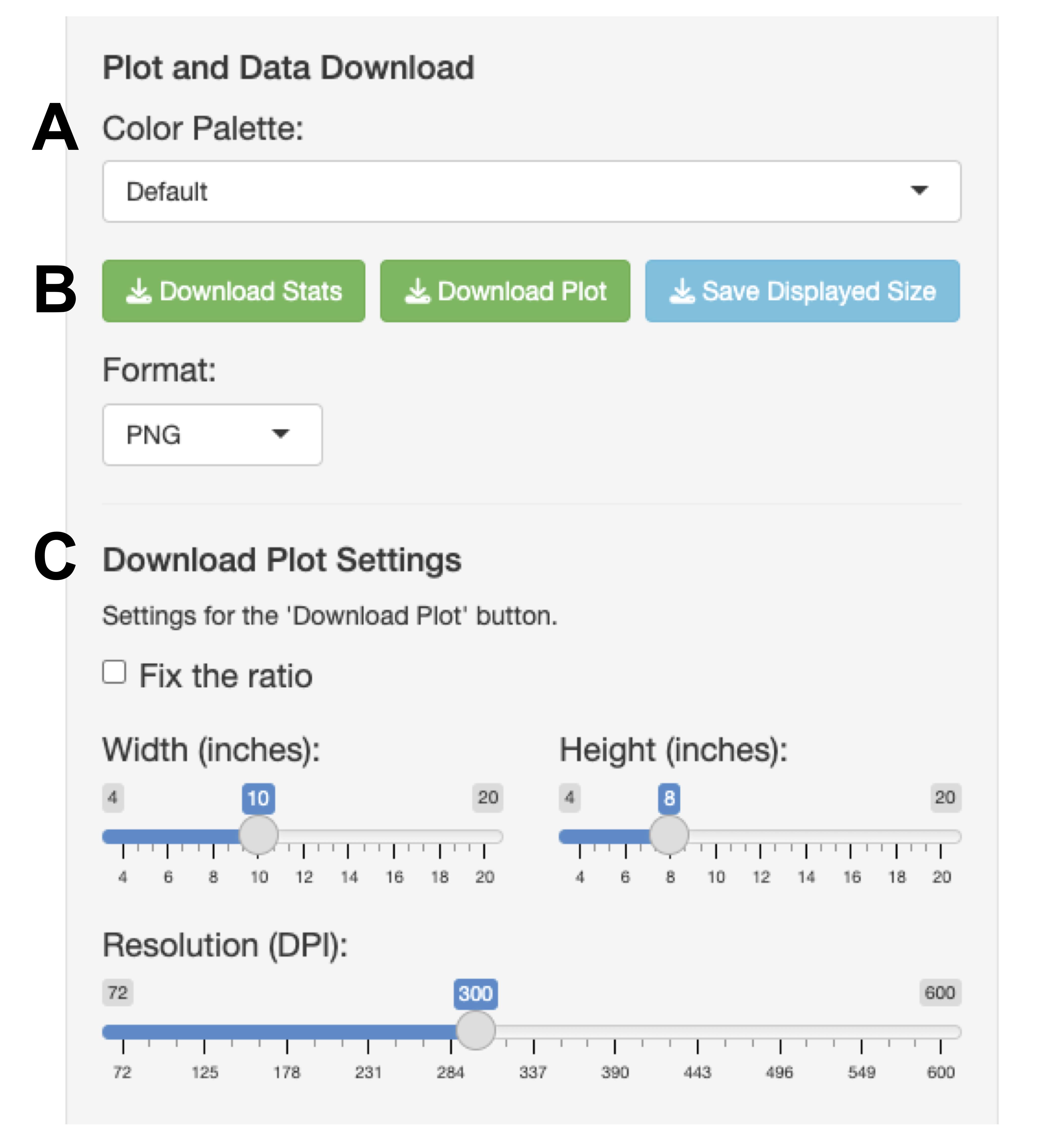
Figure 5. Area of color palette and download plot settings. (A) Color palette menu for plot. (B) Download buttons area. (C) Download plot settings panel.

Result interpretation

Data processing and statistical analysis

For the ΔCq analysis, users can select one or multiple reference genes. The Cq value for each sample is calculated using the Cq value of the target gene against the mean Cq of the selected reference gene(s). Relative expression is calculated as follows:

∆ C q = C q t a r g e t - C q r e f e r e n c e

R e l a t i v e e x p r e s s i o n = 2 - ∆ C q

Welch’s t-tests are performed on the ΔCq values for each specified group pair. Cases with zero variance are identified and reported instead of using a test statistic. In the ΔΔCq analysis, ΔCq values are first obtained as above. The ΔΔCq and fold change values are computed as follows:

∆ ∆ C q = ∆ C q t r e a t m e n t - ∆ C q c o n t r o l

F o l d c h a n g e = 2 - ∆ ∆ C q

Statistical significance between the treatment and control groups is determined using Welch’s t-tests on ΔCq values.

To compare three or more groups, an ANOVA is performed, followed by Dunnett’s post-hoc test to compare each treatment group with a single control group. This analysis is also performed on the ΔCq values.

Visualization and output

The application adjusts the plot width to accommodate the number of bars and introduces a horizontal scroll bar when necessary. Plot height is similarly adjusted based on the number of significance brackets, ensuring adequate spacing between them. All analysis modes generate high-quality bar plots, displaying mean ± standard deviation (SD) with individual data points overlaid via jitter plots. Statistical comparisons are annotated using significance brackets. Significance levels are denoted as p < 0.05 (*), p < 0.01 (**), p < 0.001 (***), and ns otherwise. The corresponding summary table of statistical analysis provides the mean, SD, sample size (N), p-value, and assigned significance symbols. In the ΔΔCq analysis, a baseline of fold change is indicated by a red dashed line on the plot.

General notes and troubleshooting

General notes

Although Click-qPCR provides an accessible and efficient platform for relative quantification analysis, several limitations should also be noted.

1. Regarding the assumption of normality, the application performs two-group comparisons using Welch’s t-tests without explicitly confirming the existence of equal variances.

2. For statistical analyses involving three or more experimental groups, the application employs a one-way ANOVA, followed by Dunnett’s multiple comparison test as the post-hoc analysis. This approach assumes both normality and homogeneity of variances across groups. The application does not test for these assumptions beforehand.

3. Simplified statistical options: The application does not offer a correction for multiple testing in two-group comparisons (e.g., Bonferroni correction or FDR), which may be relevant when analyzing many target genes simultaneously.

4. Normalization with multiple reference genes: This application supports normalization using the arithmetic mean of multiple reference genes, enhancing analysis robustness. However, automated methods for identifying stable reference genes, such as geNorm [15], NormFinder [16], and BestKeeper [17], can be conducted outside this tool.

5. No support for technical replicate handling: The input format assumes that users have average technical replicates. Raw Cq values across technical replicates must be prepared in advance.

6. Quality control of raw data: Data with very low or very high Cq values, or with amplification efficiencies outside the 90%–110% range, may be unreliable for statistical analysis. It is strongly recommended to follow quality criteria such as the MIQE guidelines [14]. This tool does not include any built-in validation step for assessing the quality of uploaded data.

Troubleshooting

Problem 1: The application is in an error state or needs to be cleared for a new dataset.

Possible cause: A previous analysis is complete, or an error has occurred during processing.

Solution: Navigate to the top of the Preprocessing and ΔCq Analysis tab and click the Reset All button to restore the application to its initial state.

Problem 2: The health of the application needs to be verified after local installation or code modification.

Possible cause: Local installation or code changes may have affected the application’s core functions.

Solution: Navigate to the Diagnostics tab and click the Run Diagnostics button (Figure 6). Confirm that all five core calculation steps (data loading, ΔCq calculation, Welch’s t-test, fold change calculation, and ANOVA/Dunnett’s test) return a Passed status.

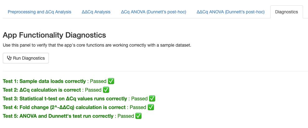
Figure 6. Example of functionality diagnostics results. Users can test the internal calculations by clicking the Run Diagnostics button.

Problem 3: How is the confidentiality of uploaded data ensured?

Solution: Click-qPCR is designed with user privacy as a top priority.

1. No server-side data storage: The application does not store or record any uploaded data on the server’s hard drive, in databases, or in any other form of permanent storage.

2. Temporary and in-memory processing: All uploaded data is processed within a temporary and isolated R session that runs in the server’s memory. All computations are performed entirely within this private environment.

3. Automatic data removal upon session termination: When the browser tab is closed or the connection to the server is interrupted, the temporary session and all associated data are automatically and permanently deleted from memory.

Problem 4: Is it possible to control the order of graphs on tabs other than the first one?

Solution: There are two ways to change the order, as follows:

1. Gene-based order: The display order on the x-axis of the graph corresponds to the order of gene names in the Target Gene(s) window (Figures 1B, 2D, 3D, and 4D), so you can rearrange the graph by changing the input order of target genes. Note that this principle applies to all tabs, including the first one.

2. Group-based order: The display order also corresponds to the order of group names in the Treatment Group(s) window, so you can rearrange the graph by changing the input order of treatment groups.

Validation of protocol

This protocol has been used and validated in the following research article:

• Kubota et al. [18]. Housing environment bilaterally alters transcriptomic profile in the rat hippocampal CA1 region. bioRxiv. (Figure 2)

Acknowledgments

Writing the original draft: A.K. Writing, review, and editing: A.T. Conceptualization: A.K. and A.T. Software: A.K. Funding Acquisition: A.K. Supervision: A.T.

This study was supported by JST SPRING (grant number JPMJSP2135). The authors thank Dr. Yasuhito Shimada and Dr. Liqing Zang for their constructive feedback, which contributed to the development of the Click-qPCR. We would like to thank Editage (http://www.editage.jp/) for English language editing.

Competing interests

The authors declare that they have no competing interests.

References

1. Harshitha, R., Arunraj, D. R. (2021). Real-time quantitative PCR: A tool for absolute and relative quantification. Biochem Mol Biol Educ. 49(5): 800–812. https://doi.org/10.1002/bmb.21552.
2. Livak, K. J., Schmittgen, T. D. (2001). Analysis of relative gene expression data using real-time quantitative PCR and the 2-ΔΔCT Method. Methods. 25(4): 402–408. https://doi.org/10.1006/meth.2001.1262.
3. R Core Team (2024). R: A Language and Environment for Statistical Computing, version 4.4.2; R Foundation for Statistical Computing, Austria. https://www.R-project.org/.
4. Chang, W., Cheng, J., Allaire, J. J., Sievert, C., Schloerke, B., Xie, Y., Allen, J., McPherson, J., Dipert, A., Borges, B. (2024). shiny: Web Application Framework for R, version 1.10.0; R Foundation for Statistical Computing, Austria. https://CRAN.R-project.org/package=shiny.
5. Attali, D. (2022). shinyjs: Easily Improve the User Experience of Your Shiny Apps in Seconds, version 2.1.0; R Foundation for Statistical Computing, Austria. https://deanattali.com/shinyjs/.
6. Wickham, H., Hester, J., Bryan, J. (2024). readr: Read Rectangular Text Data, version 2.1.5; R Foundation for Statistical Computing, Austria. https://readr.tidyverse.org.
7. Wickham, H., François, R., Henry, L., Müller, K., Vaughan, D. (2023). dplyr: A Grammar of Data Manipulation, version 1.1.4; R Foundation for Statistical Computing, Austria. https://dplyr.tidyverse.org.
8. Wickham, H. (2016). ggplot2: Elegant Graphics for Data Analysis. Springer-Verlag, New York. https://ggplot2.tidyverse.org.
9. Wickham, H., Vaughan, D., Girlich, M. (2024). tidyr: Tidy Messy Data, version 1.3.1; R Foundation for Statistical Computing, Austria. https://tidyr.tidyverse.org.
10. Xie, Y., Cheng, J., Tan, X. (2024). DT: A Wrapper of the JavaScript Library 'DataTables,' version 0.33; R Foundation for Statistical Computing, Austria. https://github.com/rstudio/DT.
11. Neuwirth, E. (2022). RColorBrewer: ColorBrewer Palettes, version 1.1-3. R Foundation for Statistical Computing, Austria. https://CRAN.R-project.org/package=RColorBrewer.
12. Iannone, R. (2024). fontawesome: Easily Work with 'Font Awesome' Icons, version 0.5.3; R Foundation for Statistical Computing, Austria. https://github.com/rstudio/fontawesome.
13. Hothorn, T., Bretz, F., Westfall, P. (2008). Simultaneous inference in general parametric models. Biom J. 50(3): 346–363. https://doi.org/10.1002/bimj.200810425.
14. Bustin, S. A., Ruijter, J. M., van den Hoff, M. J. B, Kubista, M., Pfaffl, M. W., Shipley, G. L., Tran, N., Rodiger, S., Untergasser, A., Mueller, R., Nolan, T., Milavec, M., Burns, M. J., Huggett, J. F., Vandesompele, J., Wittwer, C. T. (2025). MIQE 2.0: Revision of the minimum information for publication of quantitative real-time PCR experiments guidelines. Clin Chem. 71(6): 634–651. https://doi.org/10.1093/clinchem/hvaf043.
15. Vandesompele, J., De Preter, K., Pattyn, F., Poppe, B., Van Roy, N., De Paepe, A., and Speleman, F. (2002). Accurate normalization of real-time quantitative RT-PCR data by geometric averaging of multiple internal control genes. Genome Biol. 3(7): Research0034. https://doi.org/10.1186/gb-2002-3-7-research0034.
16. Andersen, C. L., Jensen, J. L., Ørntoft, T. F. (2004). Normalization of real-time quantitative reverse transcription-PCR data: a model-based variance estimation approach to identify genes suited for normalization, applied to bladder and colon cancer data sets. Cancer Res. 64(15): 5245–5250. https://doi.org/10.1158/0008-5472.CAN-04-0496.
17. Pfaffl, M. W., Tichopad, A., Prgomet, C., Neuvians, T. P. (2004). Determination of stable housekeeping genes, differentially regulated target genes and sample integrity: BestKeeper--Excel-based tool using pair-wise correlations. Biotechnol Lett. 26(6): 509–515. https://doi.org/10.1023/B:BILE.0000019559.84305.47.
18. Kubota, A., Kojima, K., Koketsu, S., Kannon, T., Sato, T., Hosomichi, K., Shinohara, Y. and Tajima, A. (2025). Housing environment bilaterally alters transcriptomic profile in the rat hippocampal CA1 region. bioRxiv.e651351. https://doi.org/10.1101/2025.04.29.651351