- Protocols

- Articles and Issues
- For Authors
- About
- Become a Reviewer

Characterizing Tissue Oxygen Tension During Neurogenesis in Human Cerebral Organoids
(*contributed equally to this work, § Technical contact) Published: Vol 15, Iss 22, Nov 20, 2025 DOI: 10.21769/BioProtoc.5507 Views: 1715
Reviewed by: Sébastien GillotinAbhishek VatsSreesankar Easwaran
Original research article
The authors used this protocol in:

Mar 2025

Protocol Collections
Comprehensive collections of detailed, peer-reviewed protocols focusing on specific topics


Abstract
Oxygen tension is a key regulator of early human neurogenesis; however, quantifying intra-tissue O2 in 3D models for an extended period remains difficult. Existing approaches, such as needle-type fiber microsensors and intensity-based oxygen probes or time-domain lifetime imaging, either perturb the organoids or require high excitation doses that limit the measurement period. Here, we present a step-by-step protocol to measure intra-organoid oxygen in human cerebral organoids (hCOs) using embedded ruthenium-based CPOx microbeads and widefield frequency-domain fluorescence lifetime imaging microscopy (FD-FLIM). The workflow covers dorsal/ventral cerebral organoid patterning, organoid fusion at day 12 with co-embedded CPOx beads, standardized FD-FLIM acquisition (470-nm external modulation, 16 phases at 50 kHz, dual-tap camera), automated bead detection and lifetime extraction in MATLAB, and session-matched Stern–Volmer calibration with Ru(dpp)3(ClO4)2 to convert lifetimes to oxygen concentration. The protocol outputs per-bead oxygen maps and longitudinal patterns stratified by bead location (intra-organoid vs. gel) and sample state (healthy vs. abnormal), enabling direct linkage between developmental growth and oxygen dynamics.
Key features
• End-to-end workflow linking hCOs generation, on-gel bead embedding, and FD-FLIM oxygen readout.
• Longitudinal single-organoid tracking of oxygen tension with bead-level metadata.
• Reference-based lifetime calibration and reproducible camera/LED settings.
• Ready-to-reuse materials, recipes, timing, and analysis logic.
Keywords: Human cerebral organoidGraphical overview
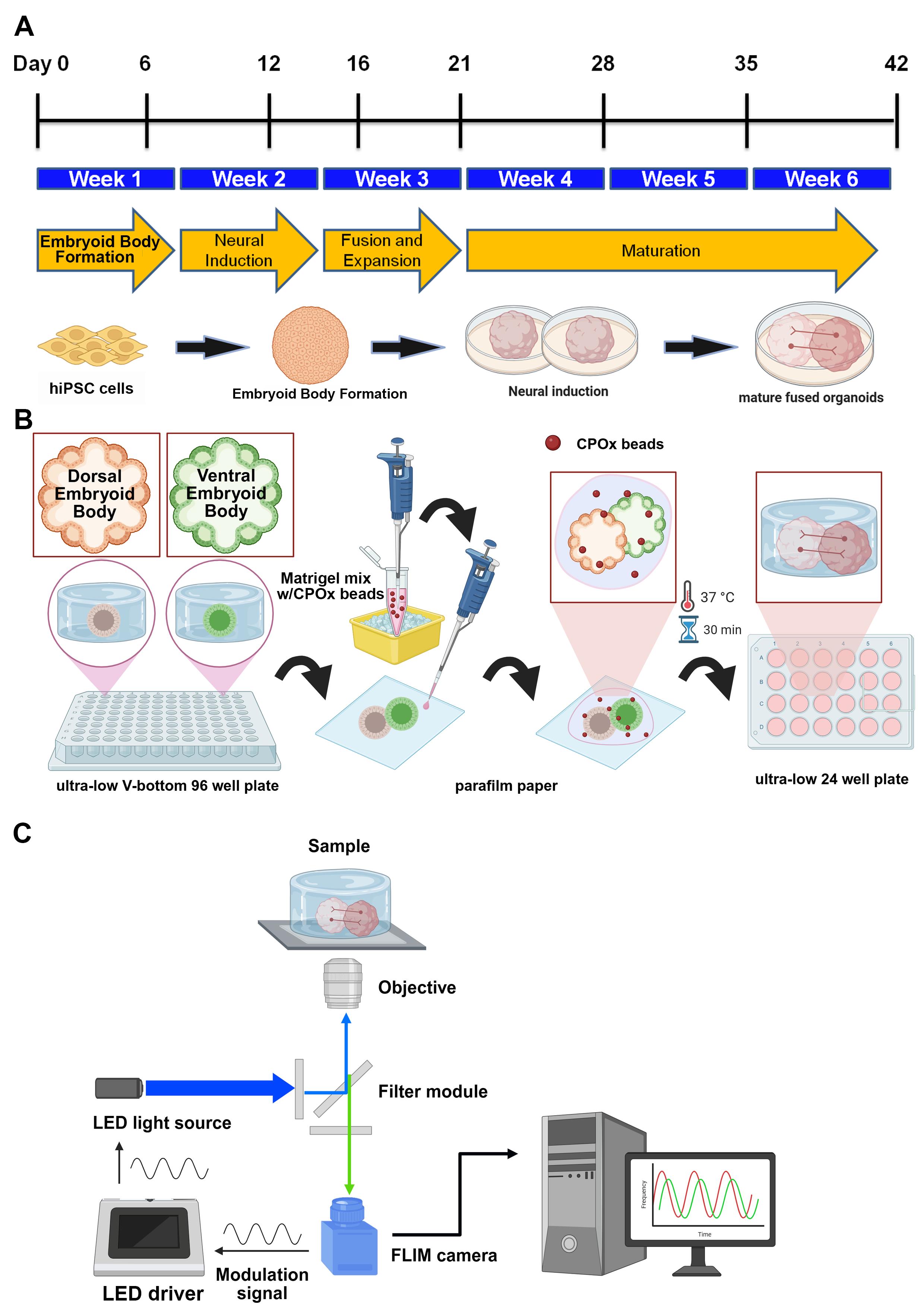
Workflow and timeline for fused human cerebral organoids (hCOs) generation. (A) Experimental timeline of dorsal/ventral embryoid bodies (EBs) patterning from human induced pluripotent stem cells (hiPSCs). Cerebral organoids were fused at day 12 and cultured for up to six weeks. (B) Schematic illustration for the incorporation of CPOx microbeads (oxygen sensor) during organoids fusion. (C) Schematic illustration for oxygen tension measurement through frequency-domain fluorescence lifetime microscopy (FD-FLIM).
Background
Oxygen availability is a central regulator of neural development, shaping stem/progenitor proliferation, neuronal differentiation, and metabolic state in the embryonic cortex [1–4]. Direct, longitudinal measurement of tissue oxygen in the developing human brain has been technically prohibitive. Human cerebral organoids (hCOs) offer an accessible, human-relevant platform to interrogate oxygen dynamics over time [5,6] and have been widely applied across neurological disease modeling contexts [6–8].
Approaches to monitor intra-organoid oxygen include needle-type optical fiber microsensors [6], which provide spatial oxygen profiles but are disruptive and unsuitable for repeated measurements over weeks. Non-disruptive, lifetime-based optical methods using oxygen-sensitive probes with phosphorescence lifetime imaging microscopy (PLIM)/fluorescence lifetime imaging microscopy (FLIM) mitigate intensity and ambient-noise confounds [9,10]. However, conventional time-domain lifetime implementations often require high excitation doses that risk photocytotoxicity in long-term live imaging, which makes it disadvantageous for live organoid observation over an extended period. In contrast, widefield frequency-domain (FD-FLIM) enables rapid, low-dose lifetime acquisition, making it suitable for longitudinal tracking of embedded oxygen sensors [11,12].
Building on this framework, our recent study used ruthenium-based oxygen-sensitive microbeads with FD-FLIM to identify a discrete developmental window (weeks 4–6) of markedly elevated intra-organoid oxygen tension that coincides with rapid neurogenesis and shifts in energy homeostasis [5]. Hypoxia or genetic perturbation of neuroglobin (NGB) attenuates this oxygen elevation and impairs neurogenesis, establishing a functional link between oxygen tension, metabolic programs, and developmental outcomes in hCOs. This protocol operationalizes that framework—detailing (i) hCO generation, (ii) bead co-embedding at fusion, and (iii) FD-FLIM configuration, acquisition, and analysis—so that other laboratories can reproduce longitudinal intra-organoid oxygen measurements and apply them to questions in human neurodevelopment, genetic perturbation (e.g., NGB), disease modeling, and microenvironmental manipulation.
Materials and reagents
Biological materials
1. Human induced pluripotent stem cells (hiPSCs) (RIKEN Bioresource Center, Cell No. HPS0076, clone 409B2)
Reagents
1. StemflexTM (Thermo Fisher Scientific, catalog number: A3349401)
2. Matrigel (hESC-qualified; coating) (Corning, catalog number: 354277)
3. Accumax (Sigma-Aldrich, catalog number: A7089)
4. AggreWellTM embryoid body (EB) formation medium (STEMCELL Technologies, catalog number: 05893)
5. DMEM/F12 (Thermo Fisher Scientific, catalog number: 12660012)
6. Neurobasal (Thermo Fisher Scientific, catalog number: 21103049)
7. N2 supplement (Thermo Fisher Scientific, catalog number: 17502048)
8. B27 supplement (without vitamin A) (Thermo Fisher Scientific, catalog number: 12587010)
9. B27 supplement (with vitamin A) (Thermo Fisher Scientific, catalog number: 17504044)
10. GlutaMAX (Thermo Fisher Scientific, catalog number: 35050061)
11. MEM-NEAA (Thermo Fisher Scientific, catalog number: 11140050)
12. Heparin (Sigma-Aldrich, catalog number: H0878)
13. ROCK inhibitor Y-27632 (Sigma-Aldrich, catalog number: SCM075)
14. Cyclopamine A (Sigma-Aldrich, catalog number: 239803)
15. IWP-2 (Sigma-Aldrich, catalog number: I0536)
16. SAG (Sigma-Aldrich, catalog number: 566660)
17. 2-Mercaptoethanol (Thermo Fisher Scientific, catalog number: 21985023)
18. Insulin (Sigma-Aldrich, catalog number: I9278)
19. DPBS (Ca2+/Mg2+-free) (Thermo Fisher Scientific, catalog number: 14190144)
20. Bovine serum albumin (BSA) (Sigma-Aldrich, catalog number: A9418)
21. CellMaskTM plasma membrane stains (Thermo Fisher Scientific, catalog number: C10046)
22. Ruthenium-based phosphorescent microbeads (CPOx beads) (Colibri Photonics, catalog number: CPOx-50-RuP)
23. Tris(4,7-diphenyl-1,10-phenanthroline)ruthenium(II) bis(perchlorate) [Ru(dpp)3(ClO4)2] (Toronto Research Chemicals, catalog number: TRC-T884520-500mg)
Solutions
1. Aggregation medium (see Recipes)
2. Neural Induction (NI) medium for dorsal patterning (see Recipes)
3. Neural Induction (NI) medium for ventral patterning (see Recipes)
4. CPOx beads stock solution (see Recipes)
5. CPOx-containing Matrigel solution (see Recipes)
6. hCOs expansion medium (see Recipes)
7. hCOs maturation medium (see Recipes)
Recipes
Note: The basal medium can be stored at -20 °C for six months and thawed immediately before use. However, as presented in the following recipes, all culture media can be stored for up to two weeks at 4 °C. The small molecules Y-27632, Cyclopamine A, IWP-2, and SAG should be added right before use. CPOx-containing Matrigel solution should be manipulated at 4 °C to prevent premature solidification of Matrigel.
1. Aggregation medium
| Reagent | Final concentration | Quantity or volume |
| AggreWellTM EB formation medium | 10 mL | |
| ROCK inhibitor Y-27632 (10 mM) | 10 μM | 10 μL |
2. Neural induction (NI) medium for dorsal patterning
| Reagent | Final concentration | Quantity or volume |
| DMEM/F12 medium | 10 mL | |
| GlutaMAX (100×) | 1:100 | 100 μL |
| MEM-NEAA (100×) | 1:100 | 100 μL |
| Heparin (1 mg/mL) | 1 μg/mL | 10 μL |
| N2 (100×) | 1:100 | 100 μL |
| Cyclopamine A (5 mM) | 5 μM | 10 μL |
3. Neural induction (NI) medium for ventral patterning
| Reagent | Final concentration | Quantity or volume |
| DMEM/F12 medium | 10 mL | |
| GlutaMAX | 1:100 | 100 μL |
| MEM-NEAA (100×) | 1:100 | 100 μL |
| Heparin (1 mg/mL) | 1 μg/mL | 10 μL |
| N2 (100×) | 1:100 | 100 μL |
| IWP-2 (5 mM) | 2.5 μM | 5 μL |
| SAG (10 mM) | 100 nM | 1 μL |
4. CPOx beads stock solution
| Reagent | Final concentration | Quantity or volume |
| DPBS | 1 mL | |
| CPOx (10 mg) | 10 mg/mL | |
| BSA (100%) | 1% | 10 μL |
5. CPOx-containing Matrigel solution
| Reagent | Final concentration | Quantity or volume |
| Matrigel | 100 μL | |
| CPOx beads stock solution (10 mg/mL) | 500 μg/mL | 5 μL |
6. hCOs expansion medium
| Reagent | Final concentration | Quantity or volume |
| DMEM/F12 medium | 25 mL | |
| Neurobasal | 25 mL | |
| GlutaMAX (100×) | 1:100 | 500 μL |
| MEM-NEAA (100×) | 1:200 | 250 μL |
| 2-mercaptoethanol (55 mM) | 19.25 μM | 17.5 μL |
| Insulin (10 mg/mL) | 2.5 μg/mL | 12.5 μL |
| N2 (100×) | 1:200 | 250 μL |
| B27 without vitamin A (50×) | 1:100 | 500 μL |
7. hCOs maturation medium
| Reagent | Final concentration | Quantity or volume |
| DMEM/F12 medium | 25 mL | |
| Neurobasal | 25 mL | |
| GlutaMAX (100×) | 1:100 | 500 μL |
| MEM-NEAA (100×) | 1:200 | 250 μL |
| 2-mercaptoethanol (55 mM) | 19.25 μM | 17.5 μL |
| Insulin (10 mg/mL) | 2.5 μg/mL | 12.5 μL |
| N2 (100×) | 1:200 | 250 μL |
| B27 with vitamin A (50×) | 1:100 | 500 μL |
Laboratory supplies
1. 6-well plates (Corning, catalog number: 3516)
2. Ultra-low-attachment 96-well round-bottom plates (Corning, catalog number: 7007)
3. Ultra-low-attachment 24-well plates (Corning, catalog number: 3473)
4. Microscope glass slide (Paul Marienfeld GmbH & Co. KG, catalog number: 1000000)
5. Microscope cover glass (diameter: 18 mm) (Paul Marienfeld GmbH & Co. KG, catalog number: 0111580)
Equipment
1. CO2-resistant shaker (Thermo Fisher Scientific, catalog number: 88881101B)
2. DMI6000 B inverted microscope (objective: 5×) (Leica Microsystems, catalog number: DMI6000B)
3. Hamamatsu ORCA-R2 cooled CCD camera (Hamamatsu Photonics K.K., catalog number: C10600-10B)
4. Dual-tap complementary metal-oxide semiconductor (CMOS) FLIM camera (Excelitas Technologies Corp., catalog number: PCO.FLIM)
5. High-power light-emitting diode (LED, nominal wavelength: 470 nm) (Thorlabs, catalog number: M470LP-C2)
6. LED driver (Thorlabs, catalog number: DC2200)
Software and datasets
1. Leica Application Suite X (LAS X) life science microscope software (Leica Microsystems, version: 3.4.2.18368)
2. Look@FLIM (version: 1.0.836-7, https://www.fish-n-chips.de/Look@FLIM/setup/, access date: 07/03/2025)
3. MATLAB (The MathWorks, Inc., version: 9.2.0.556344; R2017a)
4. ImageJ (U.S. National Institutes of Health)
5. SPSS (IBM Corp., version: 16)
6. Sigma plot (Grafiti, version: 14)
7. BioRender (https://app.biorender.com/)
8. AutoCAD (Autodesk Inc., version: 2020)
Procedure
Timing
• Section A: hCO generation to fusion day (day 0–12): ~12 days (EB formation through day 6; neural induction at day 6 when EBs > 500 μm; patterning day 6–12)
• Section B: Bead embedding at fusion: ~1 h hands-on
• Section C/D/E: Imaging configuration and acquisition: ~30–60 min setup; ~5–10 min per bead ROI
A. Generate human cerebral organoids (days 0–12)
1. EB formation (days 0–5):
a. Dissociate hiPSC colonies with Accumax to single cells. Seed 12,000 cells/well into ultra-low-attachment 96-well round-bottom plates in 150 μL of AggreWellTM EB formation medium with 10 μM Y-27632 (ROCK inhibitor). Do not disturb the plate for at least 24 h. After 24 h, small EBs (100–200 μm in diameter) should be observed with a layer of unincorporated cells around the central EB.
b. On days 2 and 4, exchange the media by removing ~75% of the media in each well and adding 150 μL of fresh AggreWellTM EB formation medium (without Y-27632).
Critical: Achieving uniform cell suspension and seeding density is essential for generating consistent, uniform embryoid body (EB) size, which directly impacts later neurogenesis.
2. Neural induction (days 5–12):
a. Monitor EB diameter under brightfield microscopy. When EBs exceed ~500 μm, carefully remove ~75% of the medium from each well and replace with prewarmed NI medium. Avoid disturbing the aggregates.
Note: The diameter of the EBs was directly quantified under brightfield microscopy using a calibrated ocular micrometer.
b. Continue culture in NI medium and apply regional cues:
• Dorsal identity: Add Cyclopamine A 5 μM (SHH inhibitor) for 6 days. Refresh NI with small molecules every other day.
• Ventral identity: Add IWP-2 2.5 μM (WNT inhibitor) with SAG 100 nM (SHH agonist) for 6 days. Refresh NI with small molecules every other day.
Critical: EBs that grow irregular, non-circular/elliptical shapes or fail to generate an expanded radialized neuroepithelium should be discarded.
3. Fusion (day 12):
a. Embed one dorsal EB with one ventral EB together in a single cold Matrigel droplet (see Section B for optional CPOx addition).
b. Transfer to ultra-low-attachment 24-well plates with hCOs expansion medium.
c. After 4 days of stationary culture, switch to hCOs maturation medium and place on a shaker for maturation.
Critical: Place the 24-well plate on an orbital shaker inside the incubator. Set the shaker speed to 90–100 rpm [6–8] to ensure adequate nutrient exchange and oxygen delivery without causing excessive shear stress to the developing organoids.
B. Embed CPOx beads at the time of fusion (day 12)
1. Thaw Matrigel on ice. Prepare CPOx bead stock solution at 10 mg/mL (DPBS with 1% BSA). Keep on ice.
2. Mix bead stock 1:20 (v/v) with cold Matrigel immediately (CPOx-containing matrigel) prior to fusion.
3. In a single Matrigel droplet, co-embed one dorsal EB with one ventral EB with bead-mixed Matrigel. Position organoids so that the neuroepithelial surfaces oppose and gently touch to promote tissue continuity; avoid bubbles. Polymerize for ≥30–40 min at 37 °C.
Caution: Matrigel must be kept on ice at all times before polymerization. Premature solidification will prevent proper embedding and fusion.
C. Basic configuration settings for FD-FLIM imaging acquisition
1. PCO.FLIM camera setup:
a. Switch on the camera and launch the Look@FLIM control and acquisition software on the connected workstation.
b. Once the camera is detected and operational, Look@FLIM enables control via the Camera menu.
c. Navigate to the SEQUENCE CONFIGURATION tab. This tab contains three configuration sections:
In the Modulation section:
• Under Source Select, choose Internal to configure the internal direct digital synthesizer to generate modulation signals.
• Under Output Waveform, select Sinusoidal to produce a sinusoidal modulation output from the camera.
• Set the Master Frequency to 50 kHz, optimized for lifetime measurements of CPOx beads.
• Leave Relative Phase at its default value (0°) to avoid manual phase offset adjustments between the camera’s modulation signal and any external output.
In the Phase Sequence section:
• Set Phase Number to 16, which captures 16 evenly spaced phase points across one full 360° modulation cycle.
Note: Available options are 2, 4, 8, and 16; higher phase numbers improve waveform fidelity.
• Set Phase Symmetry to Singular, so that only one phase sequence is acquired.
• Set Tap Select to Both, enabling readout from both tap A and tap B for enhanced signal quality.
In the Image Processing section:
• Under Asymmetry Correction, select No to disable internal asymmetry correction by the camera.
• Adjust the Exposure Time (in milliseconds) to ensure adequate fluorescence signal intensity.
Note: Refer to the next section of the protocol for optimal exposure time guidance based on fluorophore brightness and sample conditions.
2. LED illumination setup:
a. Connect the high-power LED to the LED driver using the SMA connector located on the rear panel of the driver.
b. Switch on the LED driver.
c. Set the LED driver to External Modulation Mode by selecting the corresponding function on the front panel. In this mode, the sinusoidal modulation signal is supplied externally by the PCO.FLIM camera.
Note: The external voltage signal from the FLIM camera modulates the LED current in synchrony with image acquisition, ensuring proper phase alignment.
d. During the experiment, use the "LED is OFF" button on the driver's front panel to toggle the LED light ON or OFF, as needed.
D. Reference image acquisition using an FD-FLIM camera
1. Preparation of the reference droplet:
a. Place a droplet of an oxygen-sensitive fluorescent dye of 25 μM Ru(dpp)3(ClO4)2 solution onto a microscope slide.
Note: The 25 μM Ru(dpp)3(ClO4)2 solution was used as a reference standard for calculating the lifetimes of the oxygen-sensitive beads. Because instrumental artifacts—such as sensor nonlinearity and limited dynamic range—can arise from the electronic and optical setup, a relative measurement against a sample with a known fluorescence lifetime was performed. This reference measurement corrects for system-dependent deviations and ensures more accurate lifetime determination of the CPOx beads.
b. Gently cover the droplet with a microscope cover glass to seal the sample.
2. Microscope setup:
a. Launch the Leica LAS X life science imaging software to control the stage and imaging parameters of the inverted microscope.
b. Set the objective lens to 5× magnification.
c. Use the following filter settings: excitation (Ex): 420–490 nm and emission (Em): 570–670 nm.
3. Focusing: Adjust the stage to focus on the bottom surface of the Ru(dpp)3(ClO4)2 dye droplet for consistent imaging.
4. Reference image acquisition: Use the Look@FLIM software to acquire a fluorescence image set across multiple phase angles using the PCO.FLIM camera. This image set will serve as the FD-FLIM reference image set for subsequent lifetime analysis.
Caution: Ensure that the selected field of view (FOV) is free of defects or artifacts.
Note: To confirm system stability, acquire several reference image sets at different positions on the sample and check their phasor plots. Refer to the “Oxygen level calculation” section of Data analysis) for details on phasor plot interpretation.
E. CPOx image acquisition using an FD-FLIM camera
1. Sample preparation: Place the 24-well plate containing the organoids with embedded CPOx beads onto the microscope stage.
2. Microscope setup (a schematic of the instrument setup for FD-FLIM is shown in Figure 1A):
a. Use the microscope control software, LAS X, to position the target organoid within the field of view (FOV).
b. Focus the objective lens precisely on the target organoid.
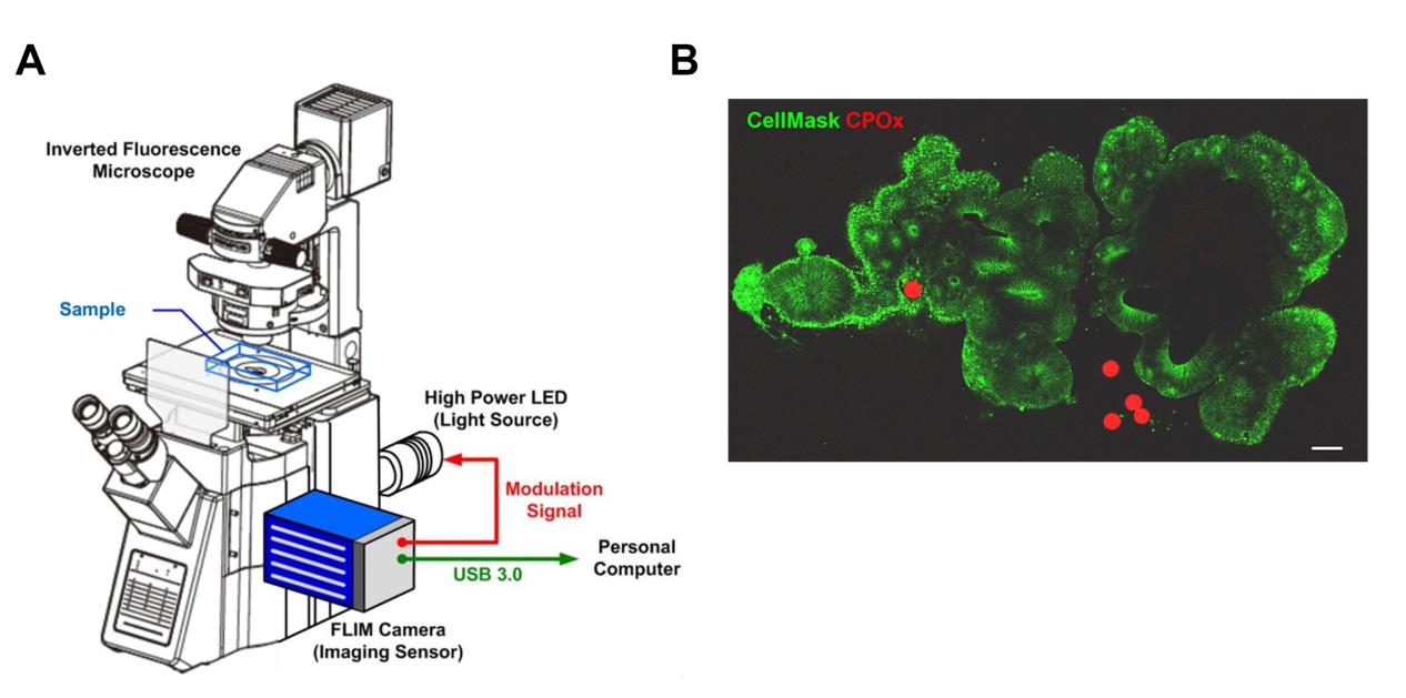
Figure 1. Instrument setup for frequency-domain fluorescence lifetime imaging microscopy (FD-FLIM) and confocal image for validation of CPOx bead localization in human cerebral organoids (hCOs). (A) Schematic of the inverted widefield frequency-domain FLIM system used for live oxygen measurements. The setup includes a 470-nm high-power LED under external modulation, an inverted fluorescence microscope with appropriate excitation/emission filters (Ex 420–490 nm/Em 570–670 nm), and a dual-tap FLIM camera for multi-phase acquisition. (B) Confocal image of a cerebral organoid after 26 days in culture, stained with CellMask (green) to delineate tissue architecture and to localize the oxygen-sensitive CPOx microbeads (red). Scale bar: 100 μm.
3. Live-cell imaging: Acquire a live-cell fluorescence image set using the Leica DMI6000 B inverted microscope equipped with a Hamamatsu monochrome CCD camera. Use filter settings as follows: excitation (Ex): 420–490 nm, Emission (Em): 570–670 nm for CPOx beads and Ex: 608–648 nm, Em: 672–712 nm for CellMaskTM plasma membrane stain.
4. FD-FLIM image acquisition:
a. Based on the live-cell image set, confirm the location of the organoids through CellMask staining and identify the target CPOx beads (Figure 1B).
b. For each CPOx bead, use the Look@FLIM software to acquire a fluorescence image set across multiple phase angles using the PCO.FLIM camera.
c. Repeat this step until all FLIM image sets of the identified CPOx beads are collected.
Caution: For each image set, record and label the following metadata:
i. Time point
ii. Organoid ID
iii. CPOx bead ID(s)
iv. Bead location (e.g., inside organoid or in gel matrix)
v. (Tip) To ensure accurate tracking and future validation, it is recommended to label each CPOx bead in the live-cell image set using bead numbers or ROI markers.
5. Longitudinal image sets: Repeat steps E2–4 every 3 or 7 days, depending on the experimental schedule, until FD-FLIM image sets have been acquired for all intended time points.
Data analysis
Organoid size quantification
Brightfield images were imported into ImageJ software and calibrated using the embedded scale bar. Each organoid was segmented by global thresholding with manual refinement as needed. For each sample, the area was calculated and recorded through the built-in measurement function of ImageJ.
Organoids were classified as healthy hCOs or abnormal hCOs. Brightfield images (Figure 2B) show that healthy hCOs exhibit smooth contours and progressive enlargement across the indicated culture days [5], whereas abnormal hCOs display irregular morphology and limited size increase. The specific characteristics defining abnormal morphology were visually detailed in Figure 2C, which included crop images highlighting two primary defects: extended, excessive cell processes or protrusions (Figure 2C') and irregular, non-smooth boundaries or a failure to form a cohesive, spherical structure (Figure 2C''). Furthermore, the quantitative summary (Figure 2D) demonstrates that healthy hCOs were consistently larger than abnormal hCOs after week 4. This analysis provides an orthogonal growth readout to validate the correlation between organoid growth and intra-organoid oxygen tension measured by the FD-FLIM/CPOx system.
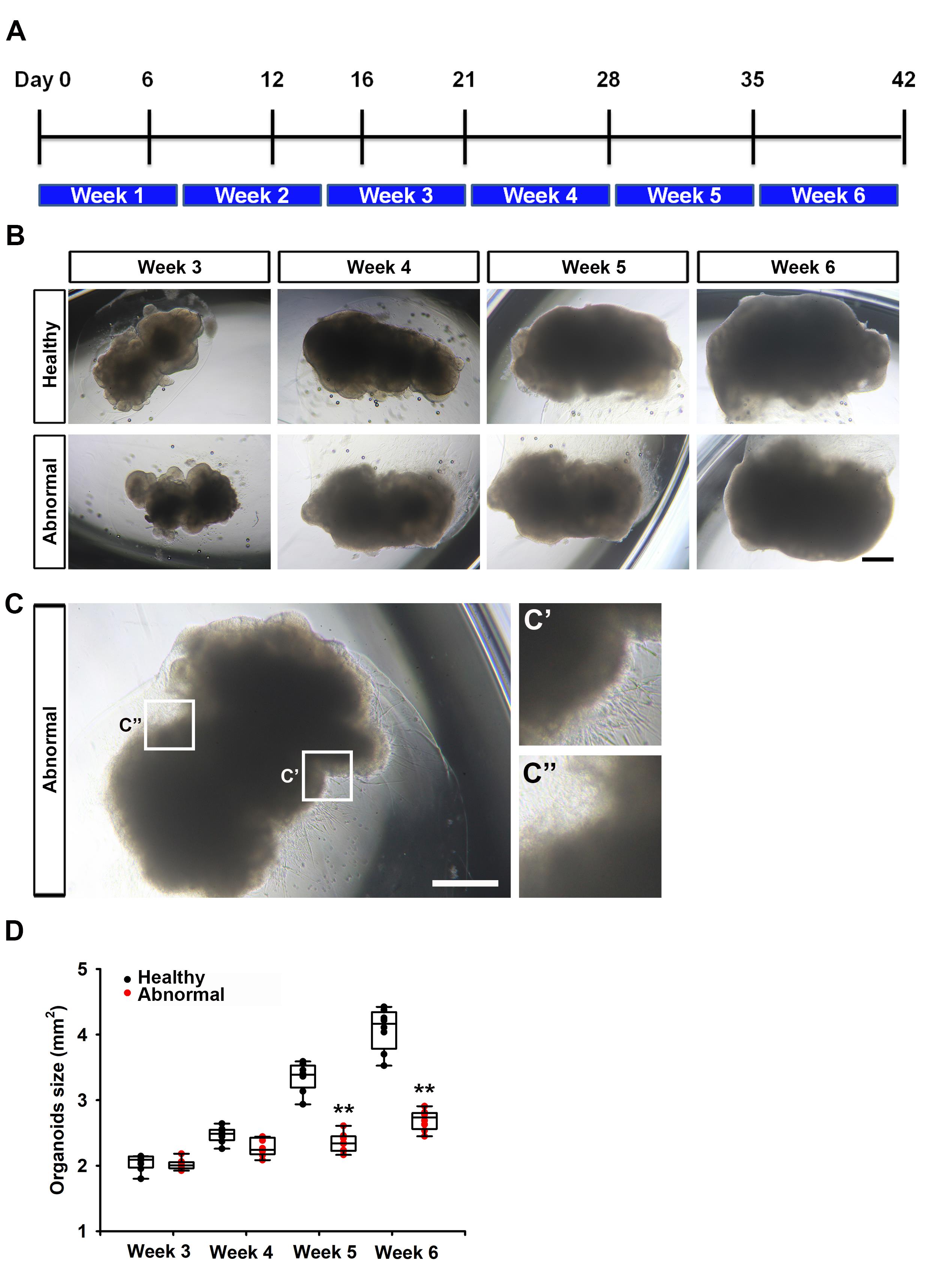
Figure 2. Timeline of human cerebral organoid (hCO) culture and size analysis. (A) Timeline of hCO formation and culture based on the fused cerebral organoid method. (B) Brightfield images of healthy and abnormal hCOs cultured in the Matrigel matrix at different time points (scale bar, 400 μm). (C) Representative brightfield images showcasing the morphological characteristics of abnormal hCOs (scale bar, 400 μm). Crop images from Figure 2C further illustrate these abnormalities: (C') highlights organoids with extended, excessive cell processes or protrusions, and (C'') displays organoids exhibiting irregular, non-smooth boundaries or a failure to maintain a cohesive, spherical structure. (D) Organoid sizes of the hCOs estimated from the captured brightfield images. Data are presented as box plots and mean ± SD with all data points (n = 8).
Oxygen level calculation
The positions of the oxygen-sensitive CPOx beads were identified using a custom MATLAB script (R2017a, MathWorks, Natick, MA). The brightest image in the acquired FLIM dataset was first binarized, and a best-fit circle detection algorithm was applied to locate the beads, taking advantage of their spherical geometry. This process generated an identification matrix marking the pixel locations of each bead for subsequent analysis.
Fluorescence intensity and lifetime of the CPOx beads were affected by molecular oxygen through dynamic quenching, resulting in reduced intensity and shortened lifetime. Lifetime values were calculated following previously described methods [12]. The lifetime profiles were multiplied by the identification matrix on a pixel-by-pixel basis to extract lifetime values corresponding to each bead.
Oxygen concentrations were then estimated from the lifetime variations using the Stern–Volmer equation:
where τ0 and τ are the fluorescence lifetimes in the absence and presence of oxygen, respectively, and Kq is the quenching constant determined from a prior calibration. Calibration was performed using FLIM images of an oxygen-sensitive reference dye solution [25 μM Ru(dpp)3(ClO4)2] with a known lifetime (τ = 1.185 μs). From these calculations, the average lifetime and oxygen concentration of each CPOx bead were obtained. The detailed procedures for bead characterization and calibration are described in the referenced literature, with step-by-step information provided in the Supplementary Information [11]. Overlaid brightfield/fluorescence images (Figure 3A) show CPOx beads (red) distributed in the matrigel and embedded within healthy hCOs. Quantitative results (Figure 3B, C) indicate distinct oxygen profiles among healthy hCOs (intra-organoid beads) [5], abnormal hCOs (intra-organoid beads), and gel-only beads (outside hCOs) [5]. Across the indicated weeks, intra-organoid oxygen levels in healthy hCOs were elevated during weeks 4–6, while abnormal hCOs displayed a flattened curve of oxygen tension; gel-only measurements remained comparatively stable. Data are displayed as mean ± SD and as box plots with all data points overlaid; independent t-tests were used for pairwise comparisons (n = 4; significance thresholds reported in the legend).
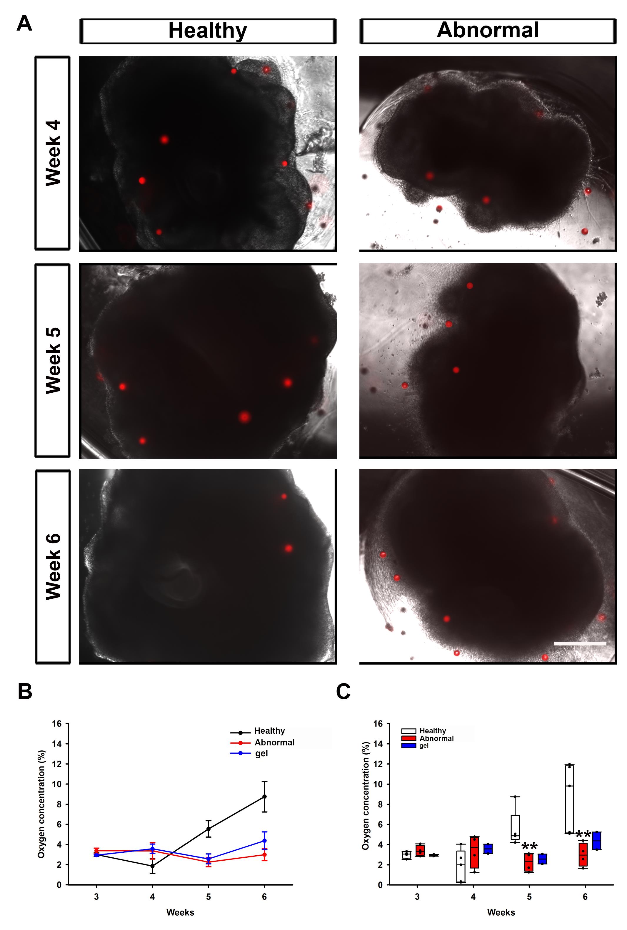
Figure 3. Healthy and abnormal human cerebral organoids (hCOs) with fluorescence oxygen-sensitive microbeads (CPOx) for intra-organoid oxygen tension measurement. (A) Overlaid brightfield and fluorescent images of the healthy and abnormal hCOs cultured with the CPOx microbeads (red) in the matrigel matrix at weeks 4, 5, and 6 (scale bar, 500 μm). (B) Quantitative results of the average oxygen tension values calculated based on the fluorescence lifetime measurement of CPOx beads embedded within the healthy and abnormal hCOs (intra-organoid oxygen tension), or within the matrigel but not embedded within the hCOs (gel oxygen tension). The data are expressed as mean ± SD. (C) Quantitative results of the average oxygen tension values across developmental time points in healthy and abnormal hCOs, as well as within the matrigel but not embedded within the hCOs (gel oxygen tension). An independent T-test was performed for statistical analysis. Data were presented as box plots and mean ± SD with all data points (n = 4, ∗p ≤ 0.05; ∗∗p ≤ 0.01).
Validation of protocol
This protocol has been used and validated in the following research article:
• Liu et al. [5]. Shaping early neural development by timed elevated tissue oxygen tension: Insights from multiomic analysis on human cerebral organoids. Sci Adv 11(11): eado1164. DOI: 10.1126/sciadv.ado1164
General notes and troubleshooting
Troubleshooting
Problem 1: Organoids fail to grow (slow growth or arrest).
Possible causes: Poor hiPSC quality (low pluripotency, mycoplasma); inaccurate seeding density or low viability at EB formation; EBs not reaching the >500 μm threshold before switching to NI; Matrigel quality/temperature issues (premature gelation or insufficient polymerization); overfilled wells limiting gas exchange.
Solutions: Verify hiPSC QC (compact colonies, high N/C ratio, mycoplasma-negative); seed 12,000 cells/well with >90% viability and maintain spherical EBs; neural induction at day 6 when EBs exceed ~500 μm; thaw Matrigel on ice carefully to avoid polymerization; avoid overfilling wells (allow gas exchange)
Problem 2: Few/no beads visible in organoids.
Possible causes: Beads settled before gelation; too low bead concentration.
Solutions: Mix bead/Matrigel gently immediately before plating; confirm a 1:20 ratio of beads to gel; minimize handling time.
Problem 3: Bead drifts between time points.
Possible causes: Mechanical disturbance; partial detachment.
Solutions: Minimize plate movement; annotate bead positions; exclude drifting beads from longitudinal statistics.
Problem 4: Organoids–Matrigel separation after embedding.
Possible cause: Strong pipetting or excessive shaking speed.
Solutions: Add medium along the well wall; avoid touching Matrigel; verify shaker speed daily.
Problem 5: Low signal-to-noise ratio (SNR) leading to poor/unstable phase fitting.
Possible causes: Insufficient excitation light dose, exposure time too short, weak sample fluorescence, suboptimal focus, or incorrect filter set.
Solutions: Increase light dose (raise LED current within safe operating limits) or extend exposure time to accumulate sufficient photons without reaching saturation; verify focus and the correct excitation/emission filters. If needed, enable pixel binning or average multiple acquisitions to further improve SNR.
Acknowledgments
Y.-H.L. and H.-M.W. conceptualized the project, performed experiments, analyzed the majority of the results, wrote the manuscript, and prepared the figures. This work was supported by the National Science and Technology Council (NSTC) Taiwan (Grant 110-2221-E-001-005-MY and 113-2313-B-002-046-MY3), Academia Sinica Career Development Award (Grant AS-CDA-106-M07), and Academia Sinica Neuroscience Core Facility (Grant AS-CFII-110-101). This protocol was used in [5]. The graphical overview was created in BioRender (https://BioRender.com/0tns243), and the schematic illustration of the inverted widefield frequency-domain FLIM system (Figure 1A) was created in AutoCAD.
Competing interests
The authors declare no competing interests.
Ethical considerations
This study has not used human or animal subjects. The usage of commercially available human induced pluripotent stem cells (RIKEN Bioresource Center, Cell No. HPS0076, clone 409B2) has been approved by the Institutional Biosafety Committee of the Academia Sinica.
References
- Lange, C., Turrero Garcia, M., Decimo, I., Bifari, F., Eelen, G., Quaegebeur, A., Boon, R., Zhao, H., Boeckx, B., Chang, J., et al. (2016). Relief of hypoxia by angiogenesis promotes neural stem cell differentiation by targeting glycolysis. EMBO J. 35(9): 924–941. https://doi.org/10.15252/embj.201592372
- Zhang, K., Zhu, L. and Fan, M. (2011). Oxygen, a Key Factor Regulating Cell Behavior during Neurogenesis and Cerebral Diseases. Front Mol Neurosci. 4: 5. https://doi.org/10.3389/fnmol.2011.00005
- Simon, M. C. and Keith, B. (2008). The role of oxygen availability in embryonic development and stem cell function. Nat Rev Mol Cell Biol. 9(4): 285–296. https://doi.org/10.1038/nrm2354
- Horie, N., So, K., Moriya, T., Kitagawa, N., Tsutsumi, K., Nagata, I. and Shinohara, K. (2008). Effects of oxygen concentration on the proliferation and differentiation of mouse neural stem cells in vitro. Cell Mol Neurobiol. 28(6): 833–845. https://doi.org/10.1007/s10571-007-9237-y
- Liu, Y. H., Chung, M. T., Lin, H. C., Lee, T. A., Cheng, Y. J., Huang, C. C., Wu, H. M. and Tung, Y. C. (2025). Shaping early neural development by timed elevated tissue oxygen tension: Insights from multiomic analysis on human cerebral organoids. Sci Adv. 11(11): eado1164. https://doi.org/10.1126/sciadv.ado1164
- Pasca, A. M., Park, J. Y., Shin, H. W., Qi, Q., Revah, O., Krasnoff, R., O'Hara, R., Willsey, A. J., Palmer, T. D. and Pasca, S. P. (2019). Human 3D cellular model of hypoxic brain injury of prematurity. Nat Med. 25(5): 784–791. https://doi.org/10.1038/s41591-019-0436-0
- Qian, X., Nguyen, H. N., Song, M. M., Hadiono, C., Ogden, S. C., Hammack, C., Yao, B., Hamersky, G. R., Jacob, F., Zhong, C., et al. (2016). Brain-Region-Specific Organoids Using Mini-bioreactors for Modeling ZIKV Exposure. Cell. 165(5): 1238–1254. https://doi.org/10.1016/j.cell.2016.04.032
- Lancaster, M. A., Renner, M., Martin, C. A., Wenzel, D., Bicknell, L. S., Hurles, M. E., Homfray, T., Penninger, J. M., Jackson, A. P. and Knoblich, J. A. (2013). Cerebral organoids model human brain development and microcephaly. Nature. 501(7467): 373–379. https://doi.org/10.1038/nature12517
- Finikova, O. S., Lebedev, A. Y., Aprelev, A., Troxler, T., Gao, F., Garnacho, C., Muro, S., Hochstrasser, R. M. and Vinogradov, S. A. (2008). Oxygen microscopy by two-photon-excited phosphorescence. Chemphyschem. 9(12): 1673–1679. https://doi.org/10.1002/cphc.200800296
- Esipova, T. V., Barrett, M. J. P., Erlebach, E., Masunov, A. E., Weber, B. and Vinogradov, S. A. (2019). Oxyphor 2P: A High-Performance Probe for Deep-Tissue Longitudinal Oxygen Imaging. Cell Metab. 29(3): 736–744 e737. https://doi.org/10.1016/j.cmet.2018.12.022
- Chang, D. M., Hsu, H. H., Ko, P. L., Chang, W. J., Hsieh, T. H., Wu, H. M. and Tung, Y. C. (2024). Rapid time-lapse 3D oxygen tension measurements within hydrogels using widefield frequency-domain fluorescence lifetime imaging microscopy (FD-FLIM) and image segmentation. Analyst. 149(6): 1727–1737. https://doi.org/10.1039/d3an01625k
- Wu, H. M., Lee, T. A., Ko, P. L., Liao, W. H., Hsieh, T. H. and Tung, Y. C. (2019). Widefield frequency domain fluorescence lifetime imaging microscopy (FD-FLIM) for accurate measurement of oxygen gradients within microfluidic devices. Analyst. 144(11): 3494–3504. https://doi.org/10.1039/c9an00143c
Article Information
Publication history
Received: Aug 31, 2025
Accepted: Oct 10, 2025
Available online: Oct 23, 2025
Published: Nov 20, 2025
Copyright
© 2025 The Author(s); This is an open access article under the CC BY-NC license (https://creativecommons.org/licenses/by-nc/4.0/).
How to cite
Readers should cite both the Bio-protocol article and the original research article where this protocol was used:
- Liu, Y. H. and Wu, H. M. (2025). Characterizing Tissue Oxygen Tension During Neurogenesis in Human Cerebral Organoids. Bio-protocol 15(22): e5507. DOI: 10.21769/BioProtoc.5507.
- Liu, Y. H., Chung, M. T., Lin, H. C., Lee, T. A., Cheng, Y. J., Huang, C. C., Wu, H. M. and Tung, Y. C. (2025). Shaping early neural development by timed elevated tissue oxygen tension: Insights from multiomic analysis on human cerebral organoids. Sci Adv. 11(11): eado1164. https://doi.org/10.1126/sciadv.ado1164
Category
Neuroscience > Development > Morphogenesis
Cell Biology > Cell imaging > Fluorescence
Biological Engineering
Do you have any questions about this protocol?
Post your question to gather feedback from the community. We will also invite the authors of this article to respond.