- Protocols

- Articles and Issues
- For Authors
- About
- Become a Reviewer

Enhancement of RNA Imaging Platforms by the Use of Peptide Nucleic Acid-Based Linkers
Published: Vol 16, Iss 9, May 5, 2026 DOI: 10.21769/BioProtoc.5453 Views: 1465
Reviewed by: Marion HoggAnonymous reviewer(s)
Original research article
The authors used this protocol in:
Feb 2025
Advertisement


Protocol Collections
Comprehensive collections of detailed, peer-reviewed protocols focusing on specific topics


Related protocols
Abstract
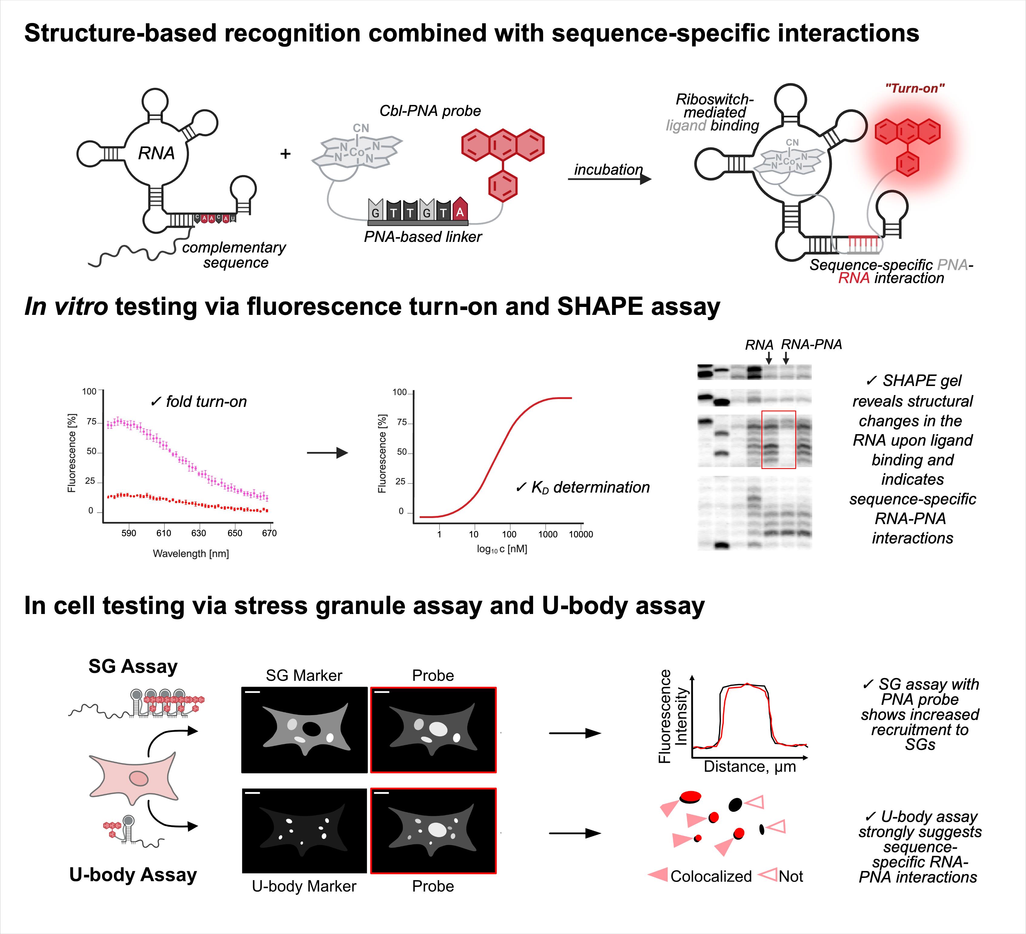
RNA imaging techniques enable researchers to monitor RNA localization, dynamics, and regulation in live or fixed cells. While the MS2-MCP system—comprising the MS2 RNA hairpin and its binding partner, the MS2 coat protein (MCP)—remains the most widely used approach, it relies on a tag containing multiple fluorescent proteins and has several limitations, including the potential to perturb RNA function due to the tag’s large mass. Alternative methods using small-molecule binding aptamers have been developed to address these challenges. This protocol describes the synthesis and characterization of RNA-targeting probes incorporating a peptide nucleic acid (PNA)-based linker within the cobalamin (Cbl)-based probe of the Riboglow platform. Characterization in vitro involves a fluorescence turn-on assay to determine binding affinity (KD) and selective 2′-hydroxyl acylation analyzed by primer extension (SHAPE) footprinting analysis to assess RNA-probe interactions at a single nucleotide resolution. To show the advancement of PNA probes in live cells, we present a detailed approach to perform both stress granule (SG) and U-body assays. By combining sequence-specific hybridization with structure-based recognition, our approach enhances probe affinity and specificity while minimizing disruption to native RNA behavior, offering a robust alternative to protein-based RNA imaging systems.
Key features
• Contains four parts, describing I) cobalamin-PNA probe synthesis, II) fluorescence turn-on assay, III) SHAPE assay, and IV) stress granule (SG) and U-body assays.
• Enables high-specificity RNA imaging through avidity, using cobalamin-based probes that incorporate peptide nucleic acid (PNA) linkers for sequence-specific hybridization with the RNA tag.
• Increases the dynamic range for the stress granule (SG) assay used in the field to evaluate a fluorescent RNA tag’s ability to visualize RNA localization.
• Provides insights on how to adapt the described procedures to other RNA-small molecule pairs.
Keywords: CobalaminGraphical overview
Background
The ability to visualize macromolecules in live cells has significantly advanced our understanding of cellular processes. While protein imaging has benefited from a wide range of genetically encoded fluorescent tags, live-cell RNA imaging remains more technically challenging and less developed. The most widely used tool for RNA visualization, the MS2-MCP system [1,2], relies on the binding of fluorescent proteins to engineered stem loops appended to the RNA of interest. Although powerful, this system suffers from several limitations, including potential perturbation of RNA function, limited signal-to-noise ratio, and challenges with multiplexing [3–5].
To address these issues, alternative RNA imaging tools have been developed that utilize RNA aptamers capable of binding small-molecule fluorophores or fluorophore-quencher conjugates. Among these, systems such as Peppers [6], RhoBAST [7], Spinach [8], Mango [9], and Riboglow [10] offer genetically encodable tags that fluoresce upon binding to their cognate ligands. Riboglow, in particular, uses a well-folding bacterial class-II cobalamin (Cbl)-binding riboswitch [11] as the RNA aptamer and a Cbl-fluorophore conjugate as the probe. In the Riboglow system, RNAs of interest are tagged with 1–4 copies of a 102-nt (33 kDa) cobalamin riboswitch that binds ~1:1 with 4.1 kDa Cbl-fluorophore probe conjugates. In contrast, the MS2-MCP system typically uses twelve or more 23-nt (7.4 kDa) MS2 stem loops that bind ~1:2 with ~40-kDa MCP-fluorescent protein conjugates. Thus, the Riboglow system introduces less total mass to an RNA of interest, potentially reducing interference with its native function. Further, upon aptamer binding, the fluorophore is spatially separated from the conjugated quencher (here, cobalamin), leading to fluorescence activation. While this system improves signal responsiveness and flexibility, its modular design has historically relied on polyethylene glycol (PEG) linkers, which are chemically inert and primarily serve as spacers.
Our recent work addresses a limitation in existing RNA imaging probe design by replacing the PEG linker in the Riboglow platform with a short peptide nucleic acid (PNA) sequence capable of base pairing with the RNA target [12]. PNAs are synthetic DNA mimics with neutral backbones, offering high binding affinity and resistance to nucleases [13]. By incorporating a six-nucleotide PNA linker complementary to a single-stranded region of the RNA aptamer (outside the Cbl-binding pocket), we introduce an additional recognition mechanism that enhances probe-RNA affinity through avidity. This dual-binding design improves affinity and enables detection of truncated aptamer variants with significantly higher sensitivity. Compared to existing methodologies, this approach offers several advantages: a) increased probe affinity through sequence-specific hybridization, b) enhanced modularity and design flexibility via tunable PNA sequences, c) improved performance in live-cell imaging, particularly in detecting RNA localized to membrane-less organelles such as stress granules (SGs), and d) compatibility with shorter or mutated RNA aptamers that would otherwise compromise probe binding [12].
The pipeline described here enables a thorough and detailed examination of the efficiency of an RNA imaging platform that combines sequence-specific hybridization with structure-based recognition. We divided the protocol into four parts (I–IV), which can be used independently or as sequential parts of the overall workflow. To enhance readability and usability, each section includes its own set of required materials, procedure description, data analysis, notes, and troubleshooting information (if applicable). We describe in detail the Cbl-PNA-based probe synthesis (Part I), in vitro testing against relevant RNA via fluorescence turn-on assay (Part II), and SHAPE gel experiments (Part III) [12]. Cell-based studies (Part IV) focus on an SG assay and a U-body assay to evaluate the ability of the Cbl-PNA probes to visualize RNA localization and dynamics [12]. The SG assay protocol described here improves upon the assay used in the field [6,10,14–20] by increasing the dynamic range of the resultant data [12]. The U-body assay protocol largely follows similar protocols already present in the literature [10,17], but we demonstrate that this assay can be used to quantify the effects of each binding mode in live cells [12].
The assays described here are not limited to Cbl probes and native cobalamin riboswitches (here, env8); they can be adapted to any RNA-probe pair. It should be noted that the in vitro fluorescence turn-on assay to determine the dissociation constant requires that the probe exhibit an increase in fluorescence upon binding to the RNA.
Part I: Cobalamin-PNA probe synthesis
Materials and reagents
Reagents
1. 1-(2-aminoethyl)-1H-pyrrole-2,5-dione, TFA salt (Ambeed, catalog number: A275035)
2. 1,1-Carbonyldi-(1,2,4-triazole) (CDT) (Chem-Impex, catalog number: 14114)
3. 6-(tritylthio)hexanoic acid (BroadPharm, catalog number: BP-25464)
4. ATTO590 alkyne (ATTO-TEC, catalog number: AD590)
5. Copper(I) iodide (CuI) (Sigma-Aldrich, catalog number: 792063)
6. Cyanocobalamin (Sigma-Aldrich, catalog number: V2876)
7. Fmoc-Lys(N3)-OH (Chem-Impex, catalog number: 29756)
8. N,N-Diisopropylethylamine (DIPEA) (Acros Organics, catalog number: 115220250)
9. PNA monomers: Fmoc-A(Bhoc)-OH (PNA Bio, catalog number: FMA-1001), Fmoc-C(Bhoc)-OH (PNA Bio, catalog number: FMC-1001), Fmoc-G(Bhoc)-OH (PNA Bio, catalog number: FMG-1001), and Fmoc-T-OH (PNA Bio, catalog number: FMT-1001)
10. Reagents for coupling reactions on the resin: 1-hydroxy-7-azabenzotriazole (HOAt) (aablocks, catalog number: AA0032PK), 2-(7-aza-1H-benzotriazole-1-yl)-1,1,3,3-tetramethyluronium hexafluorophosphate (HATU) (Ambeed, catalog number: A633512), 2,4,6-collidine (Ambeed, catalog number: A208876), 2,6-lutidine (TCI, catalog number: L0067), 4-dimethylaminopyridine (DMAP) (Ambeed, catalog number: A538667), and 4-methylmorpholine (NMM) (TCI, catalog number: M0370)
11. Reagents for Fmoc deprotection and cleavage solution: m-cresol (Sigma-Aldrich, catalog number: C85727), piperidine (Chem-Impex, catalog number: 02351), trifluoroacetic acid (Sigma-Aldrich, catalog number: T6508), triisopropylsilane (TIS) (Ambeed, catalog number: A187865)
12. Rink amide resin, 0.3–0.6 meq/g, 100–200 mesh (Chem-Impex, catalog number: 12662)
13. Solvents: acetonitrile (MeCN) (HPLC grade) (Fisher Chemical, catalog number: A998-4), dichloromethane (DCM) (Sigma-Aldrich, catalog number: 270997), diethyl ether (Et2O) (VWR, catalog number: BDH1121-1LPC), dimethyl formamide (DMF) (Acros Organics, catalog number: 348430010), dimethyl sulfoxide (DMSO) (Sigma-Aldrich, catalog number: 276855), ethyl acetate (AcOEt) (Fisher Chemical, catalog number: E145-4), H2O (HPLC grade) (Macron, catalog number: 6795-10), methanol (MeOH) (VWR, catalog number: BDH1135-4LP), N-Methyl-2-pyrrolidone (NMP) (Thermo Scientific, catalog number: 364381000), potassium phosphate monobasic buffer (pH = 7) (Fisher Chemical, catalog number: SB107-500)
14. Tris[(1-benzyl-1H-1,2,3-triazol-4 yl)methyl]amine (TBTA) (Sigma-Aldrich, catalog number: 678937)
Solutions
1. Cleavage solution (see Recipes)
2. Coupling solution (see Recipes)
3. Fmoc deprotection solution (see Recipes)
Recipes
1. Cleavage solution
Caution: TFA, TIS, and m-cresol are hazardous reagents that are corrosive, toxic, or flammable; handle them in a fume hood with appropriate personal protective equipment (PPE) and avoid inhalation or skin contact. Use a 1 oz glass bottle with a cap to store the cleavage solution.
| Reagent | Final concentration | Volume of stock |
|---|---|---|
| TFA | 95% | 5.7 mL |
| TIS | 2.5% | 150 μL |
| m-cresol | 2.5% | 150 μL |
| Total | n/a | 6 mL |
2. Coupling solution
The coupling solution is prepared using dry solvents. Follow standard dry-lab techniques when handling and transferring solvents. Store the coupling solution in a capped 2 oz glass bottle and purge with inert gas between coupling steps to preserve the solvents’ integrity. Handle solvents in a fume hood with appropriate PPE.
| Reagent | Final concentration | Volume of stock |
|---|---|---|
| DMF | 50% | 10 mL |
| NMP | 50% | 10 mL |
| Total | n/a | 20 mL |
3. Fmoc deprotection solution
The Fmoc deprotection solution is prepared using dry DMF. Follow standard dry-lab techniques when handling and transferring solvents. Store the solution in a capped 6 oz glass bottle and purge with inert gas between deprotection steps to preserve the solvents’ integrity.
Caution: Piperidine is toxic, volatile, and corrosive; handle it in a fume hood with appropriate PPE.
| Reagent | Final concentration | Volume of stock |
|---|---|---|
| DMF | 80% | 64 mL |
| Piperidine | 20% | 16 mL |
| Total | n/a | 80 mL |
Laboratory supplies
1. C18-reversed phase silica gel, LiChroprep RP-18 25-40 μm (Millipore Sigma, catalog number: 1.09303.0100)
2. Conical tubes 15 mL (VWR, catalog number: 89039-664)
3. Conical tubes 50 mL (VWR, catalog number: 89039-656)
4. Cotton wool (any reputable vendor)
5. Microcentrifuge tubes 1.5 mL (VWR, catalog number: 20170-038)
6. Microcentrifuge tubes 2 mL (VWR, catalog number: 20170-022)
7. Needles (BD PrecisionGlide, catalog number: 305167)
8. Nitrogen, compressed (Airgas, catalog number: NI UHP300)
9. Oil bath with mineral oil (Fisher Scientific, catalog number: O122-1)
10. Parafilm (Millipore Sigma, catalog number: P7793)
11. Pasteur pipettes (Millipore Sigma, catalog number: Z627992)
12. Pasteur pipette bulbs (Millipore Sigma, catalog number: Z111597)
13. Polypropylene syringes for peptide synthesis equipped with a filter and cap (Peptideweb, catalog number: PPV012L and PPVLC1)
14. Sterile, filtered, low-retention pipette tips: 1,000 μL (VWR, catalog number: 76322-154), 200 μL (VWR, catalog number: 76322-150), 10 μL (VWR, catalog number: 76322-528), 20 μL (VWR, catalog number: 76322-134), 2 μL (VWR, catalog number: 76327-214)
15. Syringes: 50 mL (BD, catalog number: 309654), 20 mL (Chemglass, catalog number: CG-3080-08), 10 mL (Chemglass, catalog number: CG-3080-06), 5 mL (Chemglass, catalog number: CG-3080-04), 1 mL (Chemglass, catalog number: CG-3080-01)
16. Test tubes (Millipore Sigma, catalog number: Z740988)
17. Weighing paper (Fisher Scientific, catalog number: 09-898-12A)
Equipment
1. Set of adjustable micropipettes covering a range of 0.1–1,000 μL (e.g., 0.1–2 μL, 2–20 μL, 20–200 μL, 100–1,000 μL from any reputable vendor)
2. Alarm timer (Santa Cruz, catalog number: sc-201632)
3. Analytical balance (Denver Instrument, catalog number: TB-224)
4. Centrifuge and rotor for 15–50 mL conical tubes (Sorvall Instruments, RC-5B Refrigerated Superspeed Centrifuge; Piramoon Technologies, Inc., FIBERLite F15-8x50c Fixed Angle Rotor)
5. Compressed air line (integrated with laboratory fume hood system)
6. Cuvette for spectrophotometric measurement, lightpath 10 mm (Fisher Scientific, catalog number: 14-385-914B)
7. Freezer (-20 °C, any reputable vendor)
8. Glass bottles with a cap: 1 oz (ULINE, catalog number: S-20888), 2 oz (ULINE, catalog number: S-20889), 6 oz (ULINE, catalog number: S-24699), 8 oz (ULINE, catalog number: S-23396)
9. Glass vial 2 mL with a cap (Agilent, catalog numbers: 5182-0716 and 5182-0717)
10. HPLC system equipped with a UV-vis detector (Agilent Technologies, model: 1260 Infinity)
11. HPLC analytical column 100-5-C18, 250 mm × 4.6 mm (Kromasil, catalog number: K08670357)
12. HPLC semipreparative column 100-5-C18, 250 mm × 10 mm (Kromasil, catalog number: K08670648)
13. Laboratory glassware: glass adapter (Chemglass, catalog number: CG-1014-01) glass column (Chemglass, catalog number: CG-1188-10), glass stopper (Chemglass, catalog number: CG-3000-14), round bottom flask 5 mL (Chemglass, catalog number: CG-1506-80), round bottom flask 100 mL (Chemglass, catalog number: CG-1506-05), round bottom flask 250 mL (Chemglass, catalog number: CG-1506-17), Schlenk line (Chemglass, catalog number: AF-0451), Schlenk tube (Chemglass, catalog number: AF-0537-01)
14. Magnetic stirrer with hot plate (IKA, model: C-MAG HS 7)
15. Magnetic stirring bar (Chemglass, model: CG-2005-30)
16. Mini centrifuge (Benchmark, model: C1008-C)
17. Peptide shaker (Peptideweb, model: LPS360PRO)
18. Refrigerator (-4 °C, any reputable vendor)
19. Rotary evaporator (BUCHI, model: Rotavapor R-300)
20. Spectrophotometer UV-Vis (Agilent, model: Cary 60 G6860A)
21. Stainless steel laboratory spatula for weighing solid reagents (any reputable vendor)
22. Test tube rack (VWR, catalog number: 89215-778)
23. Vacuum pump (Labconoco, model: 117 A65312906)
24. Vortex mixer (Fisher Scientific, model: 02215370)
Procedure
The synthesis of an exemplary Cbl-PNA-based fluorescent probe with ATTO dye has been divided into three sections (Section A, B, and C) (Figure 1; a simplified structure of cobalamin is shown for clarity).
Critical: The synthesis of cobalamin-based probes requires preexisting experience in synthetic organic chemistry and HPLC purification techniques.
Caution: All hazardous chemicals used in this procedure must be handled and disposed of in accordance with institutional, local, and federal regulations. Synthesis should be performed in a fume hood with appropriate PPE.
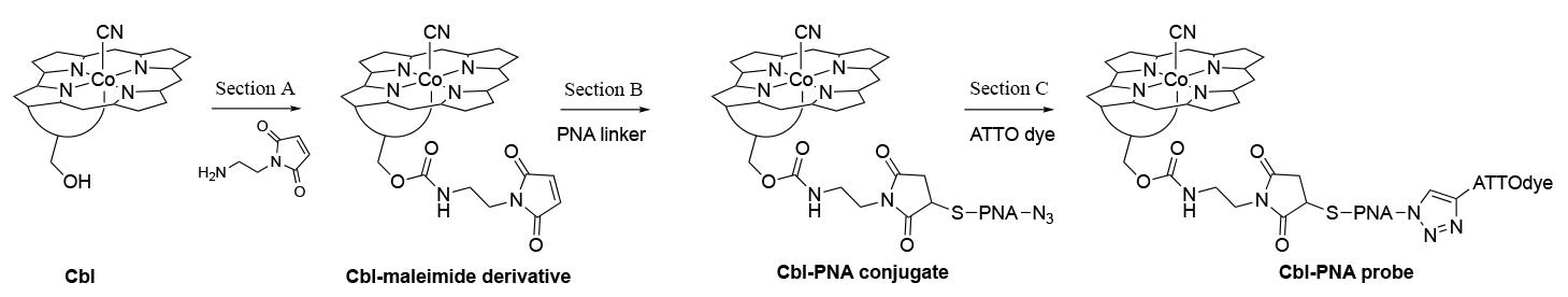
Figure 1. General scheme of Cbl-PNA-based probe synthesis
We will begin by describing the synthetic approach for the PNA linker that will be used in Section B of the synthesis (Figure 1).
Synthesis of PNA linkers bearing terminal azide and thiol groups
This procedure is adaptable to the synthesis of PNA linkers with various base compositions and terminal azide and thiol functionalities (see Figure 2). Steps 6 and 9 provide guidance on the synthesis of a 6-base PNA linker specifically for the Cbl-PNA-ATTO590 probe.
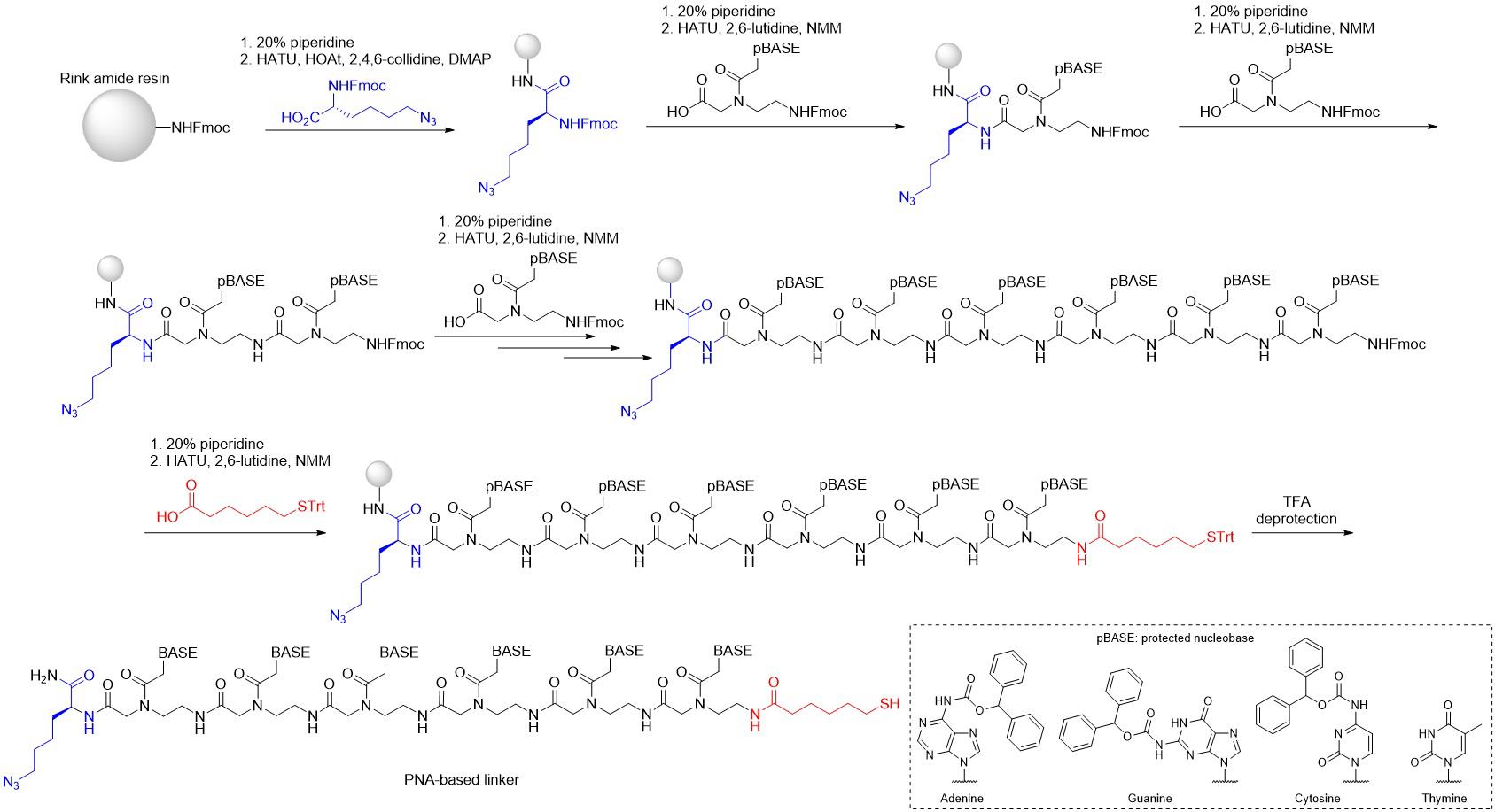
Figure 2. Synthesis of 6-base PNA linker with terminal azide and thiol functionalities (N3-PNA-SH) using Fmoc chemistry
1. Weigh 125 mg (50 μmol) of Rink amide resin into a polypropylene syringe equipped with a filter and cap.
Critical: Use a needle to aspirate any solvents or solutions into the syringe. Remove the needle whenever disposing wash residues and use a cap whenever mixing is required. Use separate needles for each solvent and solution to avoid contamination. We suggest transferring approximately 200 mL of anhydrous DMF and DCM into separate glass bottles and using them throughout the synthetic process (refill if necessary). Prepare an 8 oz glass waste bottle for collecting wash solutions.
2. Wash the resin vigorously with DCM (3 mL) and DMF (3 mL), alternating between solvents. Discard the wash solutions after each wash. Manual mixing is sufficient in this step.
3. Fmoc deprotection: Add Fmoc deprotection solution to the syringe with resin (20% piperidine in DMF, 3 mL) and mix using a peptide shaker (1 × 5 min followed by 1 × 15 min; discard the solution between washes). Wash the resin consecutively with 2× DCM, 5× DMF, and 3× DCM (between and after deprotection steps, 3 mL per wash, discard the wash solutions after each wash).
Critical: Use a timer to precisely track the duration of each step.
4. Addition of the first monomer, Fmoc-Lys(N3)-OH: Dissolve Fmoc-Lys(N3)-OH (59 mg, 3 equiv., relative to resin loading) and HATU (57 mg, 3 equiv.) in 1 mL of a DMF/NMP mixture (1:1, v/v, see Recipes) in a 2 mL microcentrifuge tube. Add HOAt (20 mg or 150 μL of 1 M DMA solution, 3 equiv.), collidine (40 μL, 6 equiv.), and a catalytic amount of DMAP (e.g., a few crystals or a small spatula tip) and vortex the tube until fully dissolved. Spin down using a minicentrifuge (3–5 s at 2,000× g), add the prepared solution to the syringe with resin, and mix for 2 h using a peptide shaker. Afterward, discard the solution and wash the resin consecutively with 3× DMF and 3× DCM (3 mL per wash, discard the wash solutions after each wash).
Note: If needed, the synthesis of the PNA linker can be paused before any Fmoc deprotection step (e.g., after steps 4, 7, or 11). Wrap the syringe tightly in Parafilm and store at 4 °C. Before resuming, rinse the resin with 3 mL of DCM followed by 3 mL of DMF.
5. Repeat step 3 above.
6. Addition of the PNA monomer: Dissolve Fmoc-PNA(Bhoc)-OH [2.5 equiv., PNA = A, C, G, or T. Critical: To synthesize PNA linker for Cbl-PNA-ATTO590, start from Fmoc-A(Bhoc)-OH monomer, 91 mg] and HATU (44 mg, 2.3 equiv.) in 1 mL of a DMF/NMP mixture (1:1, v/v) in a 2 mL microcentrifuge tube. Add NMM (14 μL, 2.5 equiv.) and 2,6-lutidine (22 μL, 3.75 equiv.) and vortex until fully dissolved. Spin down using a minicentrifuge (3–5 s at 2,000× g), add the resulting solution to the resin, and mix for 40 min using a peptide shaker. Discard the solution and wash the resin consecutively with 3× DMF and 3× DCM (3 mL per wash, discard the wash solutions after each wash).
7. Repeat step 6 to achieve maximum coupling efficiency.
8. Fmoc deprotection: Add Fmoc deprotection solution (20% piperidine in DMF, 3 mL) and shake vigorously using a peptide shaker (2 × 2 min; discard the solution between washes). Wash the resin consecutively with 2× DCM, 5× DMF, and 3× DCM (between and after deprotection steps, 3 mL per wash, discard the wash solutions after each wash).
Critical: Do not exceed 2 min of deprotection time to avoid byproduct formation. Manual mixing is sufficient during each of 2 min deprotection steps.
9. Repeat steps 6–8 until the desired PNA sequence is assembled.
Note: To synthesize 6-base PNA linker for Cbl-PNA-ATTO590, add PNA monomers in the following order: Fmoc-A(Bhoc)-OH (91 mg, 2.5 equiv.), Fmoc-T(Bhoc)-OH (63 mg, 2.5 equiv.), Fmoc-G(Bhoc)-OH (93 mg, 2.5 equiv.), Fmoc-T(Bhoc)-OH (63 mg, 2.5 equiv.), Fmoc-T(Bhoc)-OH (63 mg, 2.5 equiv.), and Fmoc-G(Bhoc)-OH (93 mg, 2.5 equiv.)
10. Addition of the last monomer, 6-(tritylthio)hexanoic acid: Dissolve 6-(tritylthio)hexanoic acid (59 mg, 3.0 equiv.) and HATU (53 mg, 2.8 equiv.) in 1 mL of a DMF/NMP mixture (1:1, v/v) in a 2 mL microcentrifuge tube. Add NMM (17 μL, 3.0 equiv.) and 2,6-lutidine (26 μL, 4.5 equiv.) and vortex until fully dissolved. Spin down using a minicentrifuge (3–5 s), add the prepared solution to the resin, and mix for 30 min using a peptide shaker. Afterward, discard the solution and wash the resin consecutively with 3× DMF and 3× DCM (3 mL per wash, discard the wash solutions after each wash).
11. Repeat step 10 to achieve maximum coupling efficiency.
Critical: Step 12 below requires ice-cold Et2O: prepare two 50 mL conical tubes with Et2O (45 mL) and chill them at -20 °C for at least 1 h prior to step 12.
12. Deprotection and cleavage from the resin: Add the cleavage solution to the syringe with resin (TFA/TIS/m-cresol, 95:2.5:2.5, v/v/v, 3 mL, see Recipes) and mix for 1 h using a peptide shaker (Caution: Use caution when handling this corrosive solution). Carefully take the cap off the syringe and transfer the resulting solution into a 50 mL conical tube containing 45 mL of ice-cold Et2O. A white pellet will precipitate. Wash the resin with the remaining 2 mL of cleavage solution (manual mixing for 30 s) and transfer this wash to the same conical tube with Et2O. Centrifuge (10 min, 6,000 rpm) and carefully discard the supernatant. Add the second portion of the ice-cold Et2O into the conical tube with the pellet and vortex vigorously for 30 s. Centrifuge (10 min, 6,000 rpm), carefully discard the supernatant, and air dry. Subsequently, transfer the pellet to a 2 mL microcentrifuge tube with spatula and dry under vacuum.
Note: The crude PNA linker has sufficient purity to be successfully used in Section B without additional purification. For HPLC purification method, see Wierzba et al. [12].
13. Confirm the molecular weight of the obtained PNA linker via mass spectrometry.
A. Synthesis of cobalamin derivative with maleimide functionality
Section A describes the first step in the synthesis of the Cbl-PNA-based probe (Figure 3).
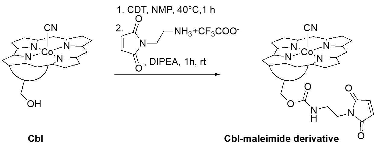
Figure 3. Synthesis of maleimide-functionalized cobalamin derivative
1. Dissolve cobalamin (70 mg, 0.05 mmol, 1 equiv.) in dry NMP (3.0 mL) in a Schlenk tube equipped with a glass stopper and a magnetic stir bar under a nitrogen atmosphere. Stir at 40 °C under a nitrogen atmosphere until fully dissolved (use oil bath and magnetic stirrer with hot plate).
Critical: Add cobalamin to the preheated solvent and wait until the cobalamin is fully dissolved before proceeding to the next step. Full dissolution usually takes approximately 5–15 min.
2. Add solid CDT (21 mg, 2.5 equiv.) to the tube under nitrogen and continue stirring at 40 °C for 1 h.
3. Remove the oil bath and allow the solution to cool to room temperature while stirring. Subsequently, add 1-(2-aminoethyl)-1H-pyrrole-2,5-dione as the TFA salt (12.7 mg, 1 equiv.) in one portion, along with DIPEA (13 μL, 1.5 equiv.), under nitrogen. Continue stirring for 1 h at room temperature (RT).
4. Transfer the reaction mixture into a 15 mL conical tube containing 10 mL of AcOEt (Note: Use a Pasteur pipette and a minimal(!) amount of MeOH to transfer any remaining residue). A red precipitate will form. Centrifuge at 4,000× g and air-dry the pellet. Redissolve it in MeOH (2–3 mL), precipitate by adding Et2O (10 mL), centrifuge at 4,000× g, and air-dry.
Critical: If the supernatant remains red, concentrate it using a rotary evaporator under reduced pressure at 40 °C. Repeat the precipitation step by dissolving the residue in MeOH (2 mL), transferring it into a 15 mL conical tube containing 10 mL of Et2O, centrifuging, and air-drying. Combine the resulting pellet with the first batch of precipitate.
5. Purify the product via reverse-phase column chromatography: Suspend 40–50 mL of C18 reversed-phase silica gel in MeOH (enough to form a gel-like suspension) and pour it into a glass column secured with cotton wool. Pack the column firmly using compressed air. Carefully exchange MeOH for H2O to prepare the column for loading. Once MeOH has been fully replaced with H2O (by passing at least three full column volumes), carefully load the crude product (dissolved in approximately 5 mL of H2O) onto the column using a Pasteur pipette. For even distribution, it is convenient to leave a 1–2 cm layer of H2O above the stationary phase and dispense the sample into this layer. After sample loading, secure the top of the column with cotton wool and elute with approximately 50 mL of H2O. Use gentle external pressure throughout the elution process. Next, replace H2O with the eluent—a mixture of MeCN and H2O, gradually increasing from 10% to 25% v/v. Adjust the gradient as needed once red band separation becomes visible. Collect the most intense red band in fractions in glass tubes.
6. Transfer the fractions containing the product into a round-bottom flask, evaporate the solvent using a rotary evaporator under reduced pressure at 40 °C, and dry under vacuum to obtain a red powder, ready for use in Section B.
B. Synthesis of cobalamin-PNA conjugate
Section B describes the second step in the synthesis of the Cbl-PNA-based probe (Figure 4). The PNA linker used in the following step is a six-base sequence, N3-ATGTTG-SH (derived from the original Cbl-PNA-ATTO590 probe) [12]. However, any other PNA linker equipped with a terminal thiol (–SH) group can be used in this step.
Figure 4. Schematic representation of Cbl-PNA conjugate synthesis
1. Dissolve the Cbl-maleimide derivative from Section A (15.2 mg, 10 μmol, 2 equiv.) in a potassium phosphate monobasic buffer (pH = 7, 650 μL) in a 2 mL centrifuge tube. Use a vortex mixer if necessary. When fully dissolved, spin down using a minicentrifuge (3–5 s at 2,000× g).
2. In a separate 2 mL centrifuge tube, dissolve the 6-base PNA linker (9.8 mg, 5 μmol, 1 equiv.) in DMSO (650 μL). Use a vortex mixer if necessary. When fully dissolved, spin down using a minicentrifuge (3–5 s at 2,000× g).
3. Combine both by adding the Cbl solution to the PNA solution and mix using a vortex mixer for 30 min.
Critical: The order of addition is crucial, as the PNA linker is insoluble in the buffer and tends to precipitate if added in reverse. Do it slowly and, preferentially, dropwise via micropipette or a Pasteur pipette.
4. Transfer the reaction mixture to a round-bottom flask and concentrate it using a rotary evaporator under reduced pressure at 40 °C.
5. Dilute the reaction mixture with MeOH (up to 5 mL), then transfer it into a 50 mL conical tube containing Et2O (45 mL). A red pellet will precipitate. Centrifuge and air-dry the pellet.
6. Purify the product via reverse-phase column chromatography.
Note: Follow the same procedure as for the purification of the Cbl-maleimide derivative, but use 30 mL of C18 reversed-phase silica gel.
7. Transfer the fractions containing the product into a round-bottom flask, evaporate the solvent using a rotary evaporator under reduced pressure at 40 °C, and dry under vacuum to obtain a red powder, ready for use in Section C.
C. Synthesis of cobalamin-PNA probe
The final step in the synthesis of the Cbl-PNA-based probe is shown in Figure 5. Here, we present the synthesis of the Cbl-PNA-ATTO590 probe, as it has been the most thoroughly tested and the most universally applicable in the cellular work presented in this protocol. Other ATTO propargylamides may be used (e.g., ATTO488 propargylamide) [12], but the synthetic step requires optimization with respect to time, temperature, and catalyst loading.
Figure 5. Schematic representation of Cbl-PNA probe synthesis
1. Prepare the catalyst solution: Dissolve CuI (1 mg, 5 μmol) and TBTA (5 mg, 10 μmol) in DMF (250 μL) in a 1.5 mL microcentrifuge tube. Stir for 20 min using a vortex mixer.
2. In a 2 mL glass vial equipped with a cap and a stir bar, dissolve the Cbl-PNA conjugate (7 mg, 2 μmol, 2 equiv., from Section B) in DMSO (20 μL), then dilute with DMF (200 μL).
Critical: DMSO is required, as Cbl-PNA conjugates exhibit poor solubility in DMF.
3. In a separate 1.5 mL microcentrifuge tube, dissolve the ATTO590 propargylamide (0.73 mg, 1 μmol, 1 equiv.) in DMF (30 μL). Use a vortex mixer if necessary. When fully dissolved, spin down using a minicentrifuge (3–5 s at 2,000× g).
4. Add the ATTO590 propargylamide solution to the solution of the Cbl-PNA conjugate.
5. Add the catalyst solution (from C1) to the Cbl-PNA conjugate solution with ATTO dye (from C4). Place the vial in an oil bath and stir at 35 °C overnight.
Note: Cover the vial with aluminum foil to protect it from prolonged light exposure.
6. Dilute the reaction mixture with MeOH (5 mL), then transfer it into a 50 mL conical tube containing Et2O (45 mL). A dark blue pellet will precipitate. Centrifuge the precipitate and air-dry.
7. Dissolve the crude product in a minimal amount of DMSO (up to 50 μL) and purify via semipreparative RP-HPLC. Conditions: column, Kromasil 100-5-C18, 250 mm × 10 mm; detection, UV/Vis (λ = 254 nm, 361 nm, and 590 nm); pressure, 20 MPa; temperature, 22 °C, flow 3 mL/min. The method is presented in Table 1.
Note: Reactions involving Cbl-PNA conjugates typically require a high catalyst loading, which leads to the formation of a byproduct in which an iodine atom is incorporated into the triazole ring. This byproduct forms alongside the desired product in approximately a 1:1 ratio. As a result, two peaks are observed on the chromatogram (at 590 nm). The first peak corresponds to the desired Cbl-PNA-ATTO590. Although the byproduct demonstrates comparable performance to the desired probe (data not shown), all experiments in Wierzba et al. [12] were conducted using the purified probe, which does not contain iodine.
Table 1. HPLC purification method for Cbl-PNA probes with ATTO590 dye
| Time (min) | H2O + 0.02% TFA | MeCN |
|---|---|---|
| Initial | 90 | 10 |
| 5 | 90 | 10 |
| 23 | 35 | 65 |
| 24 | 20 | 80 |
| 27 | 20 | 80 |
| 28 | 90 | 10 |
| 30 | 90 | 10 |
8. Transfer the fractions containing the product into a round-bottom flask, evaporate the solvent using a rotary evaporator under reduced pressure at 40 °C, and dry under vacuum to obtain a purple powder.
9. Store in a microcentrifuge tube as a solid at -20 °C or prepare DMSO aliquots for in vitro testing and cell work (see below).
To determine Cbl-PNA-ATTO590 probe concentrations:
1. Dissolve the purified pellet in 100 μL of dry DMSO.
2. Dilute the stock solution in ultrapure water using the following dilution factors: 1:500, 1:1,000, and 1:2,000.
3. Measure the absorbance of the resulting solutions using a spectrophotometer. Use ultrapure water as the blank for background subtraction.
Critical: The goal is to keep absorbance values within the linear range of A = 0.2–0.8. If the absorbance is too high, further dilute the sample accordingly. The suggested dilution factors are only a starting point and may need to be adjusted.
4. Calculate the concentration for each dilution using the Beer-Lambert law: A = ε × l × c, where ε = 120,000 M-1·cm-1 is the extinction coefficient for ATTO590 (source: ATTO-TEC), c is the concentration in mol/L, and l is the path length in cm (typically 1 cm). Average the concentrations obtained from three independent measurements to determine the concentration of the initial DMSO stock solution.
5. For fluorescence turn-on assay, dilute the initial stock to 100 μM, for the cell work, dilute the initial stock to 400 μM. Use dry DMSO.
6. Store all DMSO aliquots at -20 °C and protect from prolonged light exposure during handling.
Note: It is recommended to store all Cbl probes in dry DMSO at -20 °C. The probe stock solution can be frozen and thawed multiple times without a loss in quality. Overall, the Cbl-PNA-ATTO590 probe remains stable for an extended period (>12 months) when stored in dry DMSO at -20 °C and protected from prolonged light exposure.
Part II: Fluorescence turn-on assay
Materials and reagents
Reagents
1. 4-(2-hydroxyethyl)-1-piperazineethanesulfonic acid (HEPES) (GoldBio, catalog number: H-400-1) (1 M, pH 8.0, aqueous solution adjusted with 10 N NaOH, minimum required: 2.5 mL)
2. Cobalamin probe (here, Cbl-PNA-ATTO590, generated in-house) [12]
3. Magnesium chloride hexahydrate (MgCl2·6H2O) (Sigma-Aldrich, catalog number: 63068) (2 M, aqueous solution, minimum required: 250 μL)
4. Nonidet P-40 (Sigma-Aldrich, catalog number: N-6507) or substitute
5. Potassium chloride (KCl) (Millipore Sigma, catalog number: P3911) (4 M aqueous solution, minimum required 12.5 mL)
6. RNA of interest, 40 μM dissolved in ultrapure water (here, wild type env8 cobalamin riboswitch aptamer, env8-FL-3′antiPNA, generated in-house) [12]
7. Sodium hydroxide (NaOH) (Fisher Scientific, catalog number: S318)
8. Solvents: DMSO (Sigma-Aldrich, catalog number: 276855), ultrapure water (from Milli-Q® Benchtop Lab Water Purification System)
Solutions
1. 10× RNA buffer (see Recipes)
3. Background subtraction buffer (see Recipes)
Recipes
1. 10× RNA buffer
RNA buffer 10× is prepared using 4 M aqueous KCl stock solution, 3 M aqueous NaCl stock solution, 2 M aqueous MgCl2 stock solution, and 1 M aqueous HEPES (pH 8, adjusted with 10 N NaOH) stock solution. Use a 50 mL conical tube. After combining all reagents, mix the buffer using a vortex mixer. Store at room temperature (RT).
| Reagent | Final concentration | Volume of stock |
|---|---|---|
| KCl | 1 M | 12.5 mL |
| NaCl | 100 mM | 1.67 mL |
| MgCl2 | 10 mM | 0.25 mL |
| HEPES (pH 8) | 500 mM | 2.5 mL |
| Ultrapure H2O | n/a | 33.08 mL |
| Total | n/a | 50 mL |
2. Background subtraction buffer
Preparation of background subtraction buffer requires 10× RNA buffer (Recipe 1) and 1% aqueous Nonidet P-40 solution (prepare by adding 10 μL of 100% Nonidet P-40 into 990 μL of ultrapure water). Use a 2 mL microcentrifuge tube. After combining all reagents, mix the buffer using a vortex mixer. Store at RT.
| Reagent | Final concentration | Volume of stock |
|---|---|---|
| 10× RNA buffer | 1× | 100 μL |
| DMSO | 10% | 100 μL |
| 1% aqueous Nonidet P-40 solution | 0.01% | 10 μL |
| ultrapure H2O | n/a | 790 μL |
| Total | n/a | 1 mL |
Laboratory supplies
1. 384-well plate (Corning, catalog number: 3575) with lid (Corning, catalog number: 3935)
2. Bucket filled with crushed ice to maintain samples at 0–4 °C
3. Conical tubes 15 mL (VWR, catalog number: 89039-664)
4. Conical tubes 50 mL (VWR, catalog number: 89039-656)
5. Microcentrifuge tubes 0.6 mL (SealRite, catalog number: 1605-0099)
6. Microcentrifuge tubes 2 mL (VWR, catalog number: 490004-458)
7. Sterile, filtered, low-retention pipette tips: 1,000 μL (VWR, catalog number: 76322-154), 200 μL (VWR, catalog number: 76322-150), 10 μL (VWR, catalog number: 76322-528), 20 μL (VWR, catalog number: 76322-134), 2 μL (VWR, 76327-214)
8. Tubes 5 mL (Eppendorf, catalog number: 0030119401)
Equipment
1. Set of adjustable micropipettes covering a range of 0.1–1,000 μL (e.g., 0.1–2 μL, 2–20 μL, 20–200 μL, 100–1,000 μL)
2. Microcentrifuge tube rack (MSE Supplies, model: R1050)
3. Microplate reader (BMG Labtech, model: CLARIOstar plus)
4. Dry block heater set at 95 °C (Benchmark, model: Z742507)
5. Milli-Q® Benchtop Lab Water Purification Systems (Millipore Sigma, model: Milli-Q Biocel)
6. Mini centrifuge (Benchmark, model: C1008-C)
7. Vortex mixer (Fisher Scientific, catalog number: 02215370)
Software and datasets
1. GraphPad Prism [version 10.3.0 (507) released July 30, 2024; GraphPad Software], used for data plotting and curve fitting. This is commercial software and requires a paid license. Free alternatives include SciDAVis or LabPlot.
2. Microsoft Excel [version 16.97.2 (25052611); released May 27, 2025; Microsoft 365]. Used for background correction and normalization. This is commercial software and requires a paid license. Free alternatives include Google Sheets.
Procedure
The fluorescence turn-on assay enables the determination of the equilibrium dissociation constant KD and the fold turn-on of the probe upon binding to RNA. Affinity is assessed by titrating increasing amounts of RNA into a solution containing a constant concentration of the Cbl probe, and KD is determined by fitting the fluorescence data to a quadratic binding equation [12]. This procedure is not limited to Cbl probes and env8 riboswitches; it can be adapted to any RNA-small molecule probe pair, provided that the probe exhibits an increase in fluorescence upon RNA binding. Depending on the expected KD range, both the probe concentration and RNA input can be adjusted without altering the overall structure of the protocol. A helpful resource for optimizing assay conditions is Jarmoskaite et al. [21], which provides guidance on selecting the appropriate regime for KD determination. Figure 6 presents the general roadmap for the fluorescence turn-on assay.
Critical: When comparing the behavior of the same probe against different sets of RNAs, we strongly recommend standardizing all RNA stock concentrations to the same level (e.g., 40 μM). Similarly, when comparing the behavior of different probes against the same RNA, we recommend bringing all probe stock concentrations to the same level (e.g., 100 μM). This helps minimize pipetting errors and ensures consistency across reactions.
Figure 6. General roadmap for the fluorescence turn-on assay. (A–C) Equipment and reagent preparation (steps 1–5 of the procedure). (D) Step-by-step overview of the experimental procedure (steps 6–14 of the procedure).
1. Prepare 16 numbered 0.6 mL microcentrifuge tubes (Figure 6A). Table 2 represents the volumes of reagents for each titration point; the calculation process is described in detail in the following steps of the procedure.
Notes:
1. This procedure describes the titration between Cbl-PNA-ATTO590 and wild-type env8 cobalamin riboswitch aptamer (env8-FL-3’antiPNA) [12].
2. Every titration point contains 1 nM of Cbl-PNA probe (here, Cbl-PNA-ATTO590), 1× RNA buffer, 0.01% of Nonidet P-40 (v/v, prevents the dye from sticking to the tubes and 384-well plate), 10% DMSO (v/v, enhances probe solubility), and variable amount of RNA (dependent on the titration point).
3. The master mix used in the procedure contains Cbl-PNA probe, RNA buffer, DMSO, and Nonidet P-40.
4. The final volume of each titration point is 120 μL, of which 55 μL is pipetted twice onto a Corning 384-well plate, resulting in two technical replicates per titration point.
5. The RNA stock concentration used in this study is 40 μM (solvent: ultrapure water), and the Cbl-PNA probe stock concentration is 100 μM (solvent: dry DMSO).
Table 2. Volumes of reagents for each titration point
| Titration point | cRNA (nM) | VRNA (μL) (stock dilution) | VH2O (μL) | VMMix (μL) | VTotal = VRNA+VH2O+VMMix |
| 1 | 0 | 0 | 15 | 105 | 120 |
| 2 | 0.01 | 3 (1:100,000) | 12 | ||
| 3 | 0.05 | 15 (1:100,000) | 0 | ||
| 4 | 0.1 | 3 (1:10,000) | 12 | ||
| 5 | 0.2 | 6 (1:10,000) | 9 | ||
| 6 | 0.3 | 9 (1:10,000) | 6 | ||
| 7 | 0.5 | 15 (1:10,000) | 0 | ||
| 8 | 0.75 | 2.25 (1:1,000) | 12.75 | ||
| 9 | 1 | 3 (1:1,000) | 12 | ||
| 10 | 1.5 | 4.5 (1:1,000) | 10.5 | ||
| 11 | 2 | 6 (1:1,000) | 9 | ||
| 12 | 3 | 9 (1:1,000) | 6 | ||
| 13 | 5 | 15 (1:1,000) | 0 | ||
| 14 | 10 | 3(1:100) | 12 | ||
| 15 | 20 | 6 (1:100) | 9 | ||
| 16 | 50 | 15 (1:100) | 0 |
2. Thaw RNA stock (here, env8-FL-3’antiPNA, 40 μM) on ice and prepare RNA dilutions in ultrapure H2O (Figure 6B).
How to calculate the volume of the RNA stock solution in each reaction (Table 2, VRNA)?
Example for titration point 16:
cRNA stock = 40 μM
VTotal = 120 μL
cRNA for point 16 = 50 nM
VRNA for point 16 = (cRNA/cRNA stock) × VTotal = [(50/1,000)/40] × 120 = 0.15 μL of RNA stock solution or 15 μL of RNA stock solution diluted at a 1:100 ratio (see VRNA in Table 2 for the RNA volumes at the remaining titration points).
Critical: The volume of the master mix (VMMix) remains constant for each titration point (Table 2). However, since different volumes of RNA dilutions are used, additional water must be added to each microcentrifuge tube to equalize the final volume of 120 μL. Use the highest RNA dilution volume as a reference (in this case, 15 μL from titration point 16). Add this amount of water (15 μL) to the first microcentrifuge tube, which contains no RNA (titration point 1). For the remaining tubes, subtract the RNA volume from 15 μL and add the resulting volume of water accordingly (see column VH2O in Table 2 for the calculated values).
How much of each RNA dilution is required?
Prepare five numbered 0.6 mL microcentrifuge tubes for RNA dilutions. Begin by preparing a 1:10 dilution of the RNA stock solution (40 μM), then perform serial 10-fold dilutions using ultrapure water to achieve the desired concentrations. Use the 1:10 dilution to prepare the 1:100 dilution and continue accordingly. Prepare 30% excess of each dilution to ensure sufficient volume for subsequent steps. Perform all dilutions in 0.6 mL microcentrifuge tubes. The required RNA volumes for the titration are summarized in Table 2.
3. Incubate the RNA dilutions (prepared in step 2) in a dry block heater preheated to 95 °C for 3 min.
4. Immediately transfer the tubes to ice and incubate for at least 10 min.
Note: Steps 3 and 4 allow for proper folding of the RNA.
5. Prepare master mix (MMix) during RNA incubation (Figure 6C). Begin by estimating the number of reactions. There are 16 titration points, but it is advisable to add extra volume in case of any repeats. Adding an extra 25% results in 20 reactions of volume 120 μL. The master mix contains Cbl-PNA probe, 10× RNA buffer, DMSO, Nonidet P-40, and ultrapure H2O.
How much probe do I need for the master mix?
cprobe stock = 100 μM (in dry DMSO)
cprobe in titration reaction = 1 nM
Vprobe stock for 20 reactions = [(cprobe in reaction/cprobe stock) × VTotal] × No of reactions = [(1/(100 × 1,000)) × 120] × 20 = 0.024 μL or 2.4 μL of probe stock solution diluted at a 1:100 ratio in dry DMSO
How much 10× RNA buffer do I need for the master mix?
The reaction contains 1× RNA buffer, and the total reaction volume is 120 μL, so in each reaction, there is 12 μL of 10× RNA buffer. Multiply 12 μL by the volume of the reactions:
V10× RNA buffer = 12 μL × 20 = 240 μL
How much DMSO do I need for the master mix?
The final DMSO concentration in the reaction is 10%, so there is 12 μL of DMSO in each 120 μL reaction, analogous to the 10× RNA buffer.
VDMSO = 12 μL × 20 = 240 μL
How much Nonidet P-40 do I need for the master mix?
Use 1% aqueous solution of Nonidet P-40. The final concentration of Nonidet P-40 in the reaction is 0.01%, so there is 1.2 μL of 1% Nonidet P-40 in each 120 μL reaction. For 20 reactions:
V1%Nonidet P-40 = 1.2 μL × 20 = 24 μL
How much ultrapure H2O do I need for the master mix?
This is the remaining amount of water to obtain the expected volume and concentrations for all the ingredients.
VH2O in the master mix for 20 reactions= [VTotal – (Vprobe stock for 20 reactions/20) – V10× RNA buffer – VDMSO – V1% Nonidet P-40 – (VRNA+VH2O)) × 20 = [120 – (2.4/20) – 12 – 12 – 1.2 – 15] × 20 = 1593.6 μL
Prepare master mix by pipetting all the required reagents into a 5 mL microcentrifuge tube in the following order: ultrapure water (1593.6 μL), 10× RNA buffer (240 μL), DMSO (240 μL), 1% Nonidet P-40 (24 μL), and Cbl probe (2.4 μL of probe stock solution diluted at a 1:100 ratio in dry DMSO). Mix thoroughly using a vortex mixer. Avoid prolonged light exposure.
6. Pipette water volumes (VH2O) into microcentrifuge tubes 1–16 according to the amounts shown in Table 2.
7. Pipette 105 μL of the master mix into each of the microcentrifuge tubes 1–16.
VMMix/reaction = VMMix/No of reactions = 2100/20 = 105 μL
Critical: Mix the master mix using a vortex mixer after every 3 microcentrifuge tubes to maintain concentration consistency. The presence of Nonidet P-40 in the master mix will cause foaming during mixing, which may result in slightly challenging pipetting. To improve reproducibility, we recommend pipetting slowly and gently once the master mix has been freshly mixed. Slow pipetting is generally recommended for all solutions containing a surfactant.
8. Spin down the RNA dilutions from step 2 using a minicentrifuge (3–5 s at 2,000× g) and pipette them into microcentrifuge tubes according to the volumes listed in Table 2 (VRNA), proceeding from tube 1 to tube 16.
9. Spin down all microcentrifuge tubes using a minicentrifuge (3–5 s at 2,000× g).
10. Mix each reaction tube using a vortex mixer, then plate 55 μL of each reaction into a 384-well plate in duplicate, proceeding from tube 1 to tube 16 (Figure 6D).
Note: See the Critical note for step 7.
11. Pipette one buffer well (55 μL) for background subtraction purposes (background subtraction buffer, see Recipes).
12. Cover the plate and incubate at room temperature in the dark for 1 h before reading.
13. Read the plate using a plate reader.
Method for CLARIOstar plus microplate reader for the probes with ATTO590: Choose Fluorescence Intensity-Spectral Scan. Scan over Emission. Wavelength settings: excitation at 590 ± 8 nm and fluorescence emission from 615 ± 10 to 675 nm (spectrum resolution = 1 nm). Download the data as an Excel file (.xlsx format).
14. Repeat steps 1–13 to obtain results in triplicate (3 × 2 technical replicates = 6).
Data analysis
Plot the data following the instructions below.
1. Background correction: subtract the fluorescence values of a correction buffer (from step 11) at each wavelength and integrate the fluorescence values over all wavelengths (summarize the fluorescence level of each titration point across the whole spectrum).
Note: Use MS Excel.
2. To combine replicates, normalize each replicate to values between 0 and 100, where 0 is the value of the lower baseline and 100 is the value of the upper baseline.
Note: Use MS Excel.
3. Plot the corrected and integrated fluorescence values versus log(cRNA[nM]) in GraphPad Prism. Choose Create XY and choose options X: Numbers, Y: Enter N replicate values in side-by-side subcolumns, where N is the number of replicates (here, N = 3 × 2 technical replicates = 6).
4. Calculate KD using the following method in GraphPad Prism: Go to Analyze data, choose XY analyses, and proceed with Nonlinear regression (curve fit). Use the quadratic binding equation with one transition to fit the data: 𝑌 = 𝑚 + (𝑛 – 𝑚) × (((𝑐 + 𝑥 + 𝐾) – 𝑠𝑞𝑟𝑡(𝑠𝑞𝑟(𝑐 + 𝑥 + 𝐾) – (4 × 𝑐 × 𝑥)))/(2 × 𝑐)), where Y is the corrected integrated fluorescence value, m is the lower baseline, n is the upper baseline, c is the probe concentration, x is the RNA concentration, and K is the KD. When defining the equation, substitute c for 1 (as probe concentration is 1 nM). Set Rules for initial values as follows: m = 200000, n = 5,000,000, K = 0.001, and Rule to Initial value, to be fit. KD values, along with error values, can be found in the Results section.
5. To calculate probe fold turn-on upon binding to the RNA, divide the fluorescence value obtained from titration point 16, at cRNA = 50 nM (for Cbl-PNA-ATTO590), by the fluorescence value obtained for the free probe (titration point 1).
Part III: SHAPE assay
Materials and reagents
Reagents
1. 4-(2-hydroxyethyl)-1-piperazineethanesulfonic acid (HEPES) (GoldBio, catalog number: H-400-1) (1 M, pH 8.0, adjusted with 10 N NaOH, minimum required: 4 mL)
2. 10× T4 polynucleotide kinase (PNK) reaction buffer (New England Biolabs, catalog number: B0201S)
3. Alconox (Sigma-Aldrich, catalog number: 242985)
4. Ammonium persulfate (APS) (Sigma-Aldrich, catalog number: A3678) (10% w/v aqueous solution, minimum required: 500 μL)
5. Boric acid (Fisher Bioreagents, catalog number: BP168)
6. Bromophenol blue (Acros Organics, catalog number: 403140100)
7. Deoxynucleotide (dNTP) solution mix (New England Biolabs, catalog number: N0447L)
8. Dideoxynucleotide triphosphates (ddNTPs) (Millipore Sigma, catalog number: 3732738001)
9. Dimethyl sulfoxide (DMSO) (Sigma-Aldrich, catalog number: 276855)
10. Dithiothreitol (DTT) (Sigma-Aldrich, catalog number: D0632)
11. Ethanol (EtOH) (Decon Labs, catalog number: 2716, 200 proof)
12. Ethylenediaminetetraacetic acid disodium salt dihydrate (EDTA) (GoldBio, catalog number: E-210) (50 mM aqueous solution, pH 8.0, adjusted with 10 N NaOH, minimum required: 10 mL)
13. Formamide (Fisher Chemicals, catalog number: F84-1)
14. Glass water repellent (Rain-X, catalog number: 800002250)
15. Glycogen (20 mg/mL) (Thermo Fisher Scientific, catalog number: R0551)
16. Hydrochloric acid (HCl) (Fisher Chemical, catalog number: A144)
17. Ligands of interest (here, Cbl-PNA conjugate, generated in-house) [12]
18. Magnesium chloride hexahydrate (MgCl2·6H2O) (Sigma-Aldrich, catalog number: 63068) (2 M, 0.2 μm sterile filtered aqueous solution, minimum required: 105 μL)
19. N-methylisatoic anhydride (NMIA) (Thermo Fisher Scientific, M25; this has been discontinued, and the replacement needs to be high purity)
20. Potassium chloride (KCl) (Millipore Sigma, catalog number: P3911) (2 M, aqueous solution) (minimum required: 65 μL)
21. Reverse transcription primer resuspended to 100 μM (IDT, custom DNA oligo 5′-GAACCGGACCGAAGCCCG-3′)
22. Reverse transcriptase Superscript III, SSII (Thermo Fisher Scientific, catalog number: 18080093)
23. RNA of interest (1 μM) (here, env8-FL-3’antiPNA with additional 5′ and 3′ sequences, called a structure cassette, generated in-house) [12]
24. SequaGel UreaGel 29:1 concentrate (National Diagnostics, catalog number: EC-828)
25. SequaGel UreaGel buffer (National Diagnostics, catalog number: EC-835)
26. SequaGel UreaGel diluent (National Diagnostics, catalog number: EC-840)
27. Sodium acetate (NaOAc) (RPI, catalog number: S22020) (3 M, 0.2 μm sterile filtered aqueous solution, minimum required: 20 μL)
28. Sodium chloride (NaCl) (Thermo Scientific, catalog number: 327300010) (3 M, 0.2 μm sterile filtered aqueous solution, minimum required: 2 mL)
29. Sodium hydroxide (NaOH) (Fisher Scientific, catalog number: S318) (10 N and 4 N, aqueous solutions, minimums required: 100 mL and 5 μL)
30. T4 Polynucleotide Kinase (PNK) (New England Biolabs, catalog number: M0201)
31. Tetramethylethylenediamine (TEMED) (Sigma-Aldrich, catalog number: T9281)
32. Tris base (GoldBio, catalog number: T-400-1)
33. Tris-HCl (Fisher Bioreagents, catalog number: BP153) (1 M pH 8.3 and 1 M unbuffered, 0.2 μm sterile filtered aqueous solutions, minimums required: 85 μL and 400 μL)
34. Ultrapure H2O (from Milli-Q® Benchtop Lab Water Purification System)
35. Xylene cyanol (Sigma-Aldrich, catalog number: X4126)
36. γ-[32P]-ATP (5 mCi) (Revvity, catalog number: BLU035C005MC)
Solutions
1. 0.5× TE pH 8.0 (see Recipes)
2. 3.33× fold buffer (see Recipes)
3. Acid stop mix (see Recipes)
4. Enzyme mix (see Recipes)
5. Stop dye (see Recipes)
6. Tris borate EDTA, TBE (4×) (see Recipes)
Recipes
1. 0.5× TE pH 8.0
Dissolve Tris base and EDTA in about 400 mL of ultrapure H2O. Adjust pH with HCl to 8.0. Bring the solution to final volume. Filter sterilize with 500 mL of 0.2 μm filter unit. Store at RT.
| Reagent | Final concentration | Quantity or volume |
|---|---|---|
| Tris base | 5 mM | 0.303 g |
| EDTA | 0.5 mM | 0.093 g |
| Ultrapure H2O | n/a | Volume to 500 mL |
2. 3.33× fold buffer
Filter sterilize with a 0.2 μm syringe filter. Store at RT.
| Reagent | Final concentration | Quantity or volume |
|---|---|---|
| HEPES pH 8.0 (1 M) | 333 mM | 3.33 mL |
| MgCl2 (2 M) | 20 mM | 100 μL |
| NaCl (3 M) | 333 mM | 1.11 mL |
| Ultrapure H2O | n/a | 5.46 mL |
| Total | n/a | 10 mL |
3. Acid stop mix
| Reagent | Final concentration | Quantity or volume |
|---|---|---|
| Unbuffered Tris-HCl (1 M) | 0.14 M | 400 μL |
| Stop Dye | 86% | 2.5 mL |
| Total | n/a | 2.9 mL |
4. Enzyme mix
It remains stable when stored at -20 °C but is not tolerant to freeze-thaw cycles. Storing 30 μL aliquots is recommended; good for 5 reactions each.
| Reagent | Final concentration | Quantity or Volume |
|---|---|---|
| KCl (2 M) | 250 mM | 62.5 μL |
| Tris HCl (1 M, pH 8.3) | 167 mM | 83.5 μL |
| dNTPs (10 mM) | 1.67 mM | 83.5 μL |
| DTT (100 mM) | 17 mM | 85.0 μL |
| MgCl2 (2 M) | 10 mM | 2.5 μL |
| Ultrapure H2O | n/a | 183 μL |
| Total | n/a | 500 μL |
5. Stop dye
| Reagent | Final concentration | Quantity or volume |
|---|---|---|
| Formamide (100%) | 67.5% | 33.75 mL |
| TBE (4×) | 0.5× | 6.25 mL |
| EDTA (50 mM, pH 8.0) | 50 mM | 10 mL |
| Bromophenol blue | 0.05% | 25 mg |
| Xylene cyanol | 0.05% | 25 mg |
| Total | n/a | 50 mL |
6. Tris borate EDTA, TBE (4×)
| Reagent | Final concentration | Quantity or volume |
|---|---|---|
| Tris base | 356 mM | 172.5 g |
| Boric acid | 356 mM | 88 g |
| EDTA | 10 mM | 15 g |
| Ultrapure H2O | n/a | Volume to 4 L |
Laboratory supplies
1. Bucket filled with crushed ice to maintain samples at 0–4 °C
2. Cling film (GLAD or any reputable vendor)
3. Conical tubes 15 mL (VWR, catalog number: 89039-664)
4. Filter unit 500 mL, 0.2 μm (Corning, catalog number: 430758)
5. General-purpose laboratory labeling tape (VWR, catalog number: 89097 series)
6. Individual PCR tubes (VWR, catalog number: 732-0548)
7. Kimwipes (KIMTECH, catalog number: 34155)
8. Luer-Lok syringe 50 mL (BD, catalog number: 309653)
9. Microcentrifuge tubes 1.5 mL (VWR, catalog number: 20170-038)
10. MicroSpin G-25 column (Cytiva, catalog number: 27532501)
11. Needle 21 G (BD, catalog number: 305165)
12. Razor blade (Staples or any reputable vendor)
13. Serological pipette 25 mL (Fisherbrand, catalog number: 13-678-11)
14. Shipping tape, 2 in wide (Scotch or any reputable vendor)
15. Sterile, filtered, low-retention pipette tips + boxes: 1,000 μL (VWR, catalog number: 76322-154), 200 μL (VWR, catalog number: 76322-150), 10 μL (VWR, catalog number: 76322-528), 20 μL (VWR, catalog number: 76322-134), 2 μL (VWR, catalog number: 76327-214)
16. Syringe filter 0.2 μm (VWR, catalog number: 28145-477)
17. Weighing papers (Fisher Scientific, catalog number: 09-898-12A)
18. Whatman 3MM Chr chromatography paper, 46 × 57 cm (Cytiva, catalog number: 3030-917)
Equipment
1. Set of adjustable micropipettes covering a range of 0.1–1,000 μL (e.g., 0.1–2 μL, 2–20 μL, 20–200 μL, 100–1,000 μL from any reputable vendor)
2. Amersham Typhoon biomolecular imager (Cytiva, catalog number: 29187191)
3. Analytical balance (Denver Instrument, model: TB-224)
4. Beaker 500 mL (Chemglass, catalog number: CG-8048-600)
5. Benchtop centrifuge (Eppendorf, model: 5424)
6. Binder clips 51 mm (Staples or any reputable vendor)
7. Central vacuum system (house vacuum)
8. Desiccator (Millipore Sigma, model: BAF424002121)
9. Dry block heater set at 90 °C (Benchmark, model: Z742507)
10. Filter flask with side arm 500 mL (Chemglass, model: CG-1550-04)
11. Freezer (-20 °C, any reputable vendor)
12. Geiger counter (Ludlum Measurements, model: 3 survey meter)
13. Gel dryer (Bio-Rad, model: 583) with water aspirator (Heidolph brinkmann, model: B-169)
14. Graduated cylinder 500 mL (Chemglass, catalog number: CG-8248-500)
15. Magnetic stirrer (IKA, model: C-MAG HS 7)
16. Owl Aluminum-Back Sequencer System, gel rig (Thermo Fisher Scientific, model: S3S)
17. pH meter (Mettler Toledo, model: SevenCompact pH/Ion S220)
18. Pipette controller (Eppendorf, model: Easypet 3 EP4430000018)
19. Plexiglass shielding (Thermo Fisher Scientific, catalog number: 6700-2418)
20. Porta trace light box (Gagne, catalog number: 1824)
21. Power supply (Bio-Rad, model: PowerPac HV Pover Supply 1645056)
22. Rubber stopper for 24/40 standard taper outer joint (any reputable vendor)
23. Rubber tubing (1/4 in. ID, 3/8 in. OD, latex or silicone, any reputable vendor)
24. Sequencing system spacer sets and glass plates: blank glass, 45 cm length × 35 cm width × 3/16 in. thickness (Thermo Fisher Scientific, catalog number: S2S-45G); notched glass, 45 cm length × 35 cm width × 3/16 in. thickness (Thermo Fisher Scientific, catalog number: S2S-45R); spacer set, 45 cm length × 1 cm width × 0.04 cm thickness (Thermo Fisher Scientific, catalog number: S2S-SA4); well comb (Thermo Fisher Scientific, catalog number: S2S-20A)
25. Stir bar (Chemglass, catalog number: CG-2001P-07)
26. Storage phosphor screen (Amersham Biosciences, model: ALT 21573)
27. Tube rack for 15/50 mL conical tubes (any reputable vendor)
28. Thermocycler (Bio-Rad, model: MJ Mini PTC 11-48)
29. Vortex mixer (Fisher Scientific, catalog number: 02215370)
Software and datasets
1. Amersham Typhoon Control Software [version 3.0.0.2 (310), 2021, Cytiva]. Used to capture images of the phosphor screen. This is commercial software and requires a paid license. Other imagers should include their own commercial software.
2. Semi-Automated Footprinting Analysis (SAFA) software (version v11b, Stanford). Used to analyze the phosphor screen image. This is a free software available at https://simtk.org/frs/?group_id=69.
Procedure
To examine RNA–PNA interactions, we employed a chemical probing method known as SHAPE (Selective 2′-Hydroxyl Acylation analyzed by Primer Extension) [22,23]. This technique utilizes small electrophilic molecules—specifically, N-methylisatoic anhydride (NMIA)—that react with the 2′-hydroxyl groups of flexible, unpaired nucleotides (Figure 7A). When a nucleotide participates in stable secondary structures, such as helices formed through base pairing, its 2′-hydroxyl group becomes less reactive to NMIA. We assessed the structural flexibility of env8 RNA in the presence and absence of Cbl-PNA conjugate by mapping NMIA reactivity via radiolabeled primer extension, followed by resolution of the resulting cDNA products on a sequencing gel (Figure 7) [12].
The procedure below outlines a general approach for performing a SHAPE assay with the Cbl-PNA conjugate and the env8 riboswitch. Here, we present an approach for testing a single ligand, but the number of ligands can be increased. The concentration of a ligand in the assay depends on KD of the RNA-ligand pair. To examine RNA structural changes induced by ligand binding, a saturating ligand concentration should be used. We recommend using a 1,000-fold KD excess to ensure saturation. This procedure can be adapted for other RNA-ligand pairs and is based on previous works [23,24].
Caution: The assay involves the handling of radioactive materials. Proper user training and the use of personal PPE, including appropriate shielding, are required.

Figure 7. General roadmap for the SHAPE assay
A. NMIA reaction
The RNA of interest will be subjected to the following set of conditions (for summary, see Table 3):
• Reaction 1–2: sequencing reactions with ddNTPs.
Note: ddNTPs are used in a sequencing (ladder) reaction to generate reference lanes that help identify the exact nucleotide positions of reverse transcriptase stops on the gel. Two sequencing (ddNTP) reactions may be sufficient for mapping, but more or fewer can be used (the second column in Table 3 represents the use of two different ddNTPs).
• Reaction 3: Control reaction without NMIA
• Reaction 4: Reaction with NMIA in the absence of ligand (provides a baseline SHAPE reactivity profile of the unbound RNA, reflecting its native structural flexibility; Figure 7A)
• Reaction 5: Reaction with NMIA in the presence of ligand, here, Cbl-PNA conjugate (reveals structural changes in the RNA upon ligand binding by highlighting differences in nucleotide flexibility compared to the unbound state; Figure 7A)
Critical: The reaction, as written, uses a final concentration of 0.1 μM RNA and 30 μM ligand (ligand concentration is dependent on RNA-ligand KD; see introduction to the Procedure above). It is recommended to use RNA stock of 1 μM in 0.5× TE (here, env8-FL-3′antiPNA with additional 5′ and 3′ sequences, called a structure cassette) [12] and 300 μM stock solution of desired Cbl ligand (here, Cbl-PNA conjugate, dissolved in dry DMSO). If you wish to use different stock concentrations of RNA and ligand, adjust the volumes of 0.5× TE and ligand solvent in Table 3 accordingly.
Table 3. Reagent volumes in NMIA reaction
| Reagent/Reaction | 1–2. ddNTPs | 3. -NMIA (DMSO) | 4. -ligand (+NMIA) | 5. +ligand (+NMIA) |
|---|---|---|---|---|
| 0.5× TE | 4 μL | 4 μL | 4 μL | 4 μL |
| RNA (1 pmol) | 1 μL | 1 μL | 1 μL | 1 μL |
| Fold buffer | 3 μL | 3 μL | 3 μL | 3 μL |
| Ligand | 0 μL | 0 μL | 0 μL | 1 μL |
| Ligand solvent | 1 μL | 1 μL | 1 μL | 0 μL |
| NMIA | 0 μL | 0 μL | 1 μL | 1 μL |
| DMSO | 1 μL | 1 μL | 0 μL | 0 μL |
| Total volume | 10 μL | 10 μL | 10 μL | 10 μL |
1. Determine the amount of RNA required. For 5 reactions (10 μL each) at 0.1 μM final concentration, prepare 5 μL of 1 μM RNA stock in 0.5× TE. Add 20% extra to account for pipetting loss, resulting in a total of 6 μL.
2. Fold the RNA of interest for all NMIA reactions (6 μL of 1 μM) in a PCR tube by incubating in a dry block heater at 90 °C for 3 min and then plunging into an ice bath for 10 min.
Note: Folding procedures may vary between RNAs. The one described here works well for env8 RNA.
3. In five individual PCR tubes, add 0.5× TE, folding buffer, ligand, and ligand solvent (here, DMSO) as specified in Table 3.
Critical: Use 1 μL of 300 μM ligand DMSO stock for reaction number 5 to obtain a final ligand concentration of 30 μM.
4. Add 1 μL of folded RNA (from step A2) to each PCR tube (from step A3) and incubate at room temperature for 10 min to allow ligand binding.
Note: Ligand binding procedures vary between RNAs. The one described here works well for cobalamin and env8 RNA.
5. Prepare the NMIA solution by dissolving the equivalent of 4.6 mg of NMIA per 200 μL of anhydrous DMSO (making 130 mM NMIA).
Critical: Prepare NMIA solution just before adding to the reactions. If prepared too much ahead of time, hydrolysis may begin and inactivate the NMIA. Ensure that DMSO is anhydrous.
Notes:
1. About 1 mg of NMIA will be sufficient for over 40 reactions.
2. 130 mM is the solubility limit for NMIA in DMSO. This concentration can be lowered if less reactivity is desired. If more reactivity is desired, increase NMIA volume in the reactions.
6. Add NMIA and DMSO (control) to appropriate reaction tubes as specified in Table 3 and incubate in a thermocycler for five NMIA half-lives at desired temperature, according to the equation:
Half-life (min) = 360 × exp[-0.102 × temperature [°C]]
Notes:
a. Five half-lives at 37 °C: 42 min (use this approach for Cbl ligands and env8 RNA).
b. Five half-lives at 25 °C: 2 h 21 min.
c. Higher temperatures will give faster reactions but may not be ideal for binding. This is where a different electrophile such as 1M7 may be desirable, as it has a shorter half-life.
Pause point: Reactions can be stored at -20 °C once the NMIA reaction is complete or can continue to reverse transcription.
B. Reverse transcription
Caution: From this point forward, radioactive materials will be used. Ensure proper training of users and proper use of PPE and protective equipment such as shielding.
1. Thaw 10× T4 PNK buffer, reverse transcription primer, and γ-[32P]-ATP.
Caution: Keep the γ-[32P]-ATP vial in its protective container.
Note: The reverse transcription primer used here has the sequence 5′-GAACCGGACCGAAGCCCG-3′, which facilitates annealing to the 3′ end of the RNA structure cassette.
2. Combine in a PCR reaction tube:
a. 1 μL of 100 μM reverse transcription primer
b. 2 μL of 10× T4 PNK buffer
c. 1 μL of γ-[32P]-ATP
d. 2 μL of T4 PNK enzyme
e. 13 μL of ultrapure H2O
3. Incubate reaction tube at 37 °C in thermocycler for 45 min.
4. Toward the end of the reaction incubation, prepare a microspin G-25 column. Mix using a vortex mixer to resuspend resin. Loosen the cap one-quarter turn and twist off the bottom closure. Place column in collection tube. Spin for 1 min at 735× g. Place column in fresh 1.5 mL microcentrifuge tube, discarding the flowthrough.
5. At end of the reaction incubation, add an equal volume of ultrapure H2O (20 μL) and apply the entire reaction volume (40 μL) to the prepared microspin G-25 column.
Critical: Pipette onto the top and center of resin, being careful not to disturb resin bed.
6. Spin the microspin G-25 column for 2 min at 735× g. The labeled reverse transcription primer will collect in the microcentrifuge tube, and the unincorporated labeled nucleotide will remain in the column.
7. Dispose used column in radiation waste.
8. Ethanol-precipitate radiolabeled reverse transcription primer. Add 200 μL of 100% EtOH, 4 μL of 3 M NaOAc, and 1 μL of 20 mg/mL glycogen to microcentrifuge tube with radiolabeled reverse transcription primer. Store at -20 °C with proper radiation protection overnight.
Pause point: Radiolabeled reverse transcription primer can be left to ethanol-precipitate at -20 °C as long as needed or until radiation decays.
9. After ethanol precipitation, pellet the radiolabeled primer. Spin for 30 min at max speed in a benchtop centrifuge at 4 °C.
10. Aspirate the liquid, leaving the pellet to dry for at least 30 min.
Caution: Liquid goes into radiation waste.
11. Resuspend radiolabeled reverse transcription primer in 200 μL of 0.5× TE.
Pause point: Resuspended radiolabeled reverse transcription primer can be stored at -20 °C until use, until radiation decays.
12. Thaw as many tubes of enzyme mix as needed (see Recipes, 5 NMIA reactions per tube if stored in 30 μL aliquots), NMIA reactions, ddNTPs, and radiolabeled reverse transcription primer on ice.
13. Add 3 μL of radiolabeled reverse transcription primer to each NMIA reaction and incubate at 65 °C for 5 min in a thermocycler. From this point, tubes should stay in the thermocycler until the end of step B20.
14. Change the thermocycler temperature to 35 °C and incubate reactions for 20 min.
Note: This anneals the primer to the RNA.
15. In the last few minutes of the 35 °C incubation above, prepare the enzyme mix (see Recipes) + reverse transcriptase (SSIII). Combine all thawed tubes of enzyme mix in one 1.5 mL microcentrifuge tube. Add 2.5 μL of SSIII per 30 μL of enzyme mix, ensuring to fully mix by pipetting. Do not use vortex mixer. This will result in 0.5 μL of SSIII per reaction.
16. At the end of the 35 °C incubation, change the thermocycler temperature to 52 °C and incubate for 1 min.
Critical: This is important for good primer extension.
17. During the 1 min 52 °C incubation, add 3 μL of ddNTPs to appropriate reactions (here, reactions 1 and 2, use ddATP and ddGTP).
18. After the 1 min 52 °C min incubation, add 6.5 μL of the enzyme mix + SSIII made in step B15 to each reaction. Mix by pipetting. Incubate at 52 °C for 5 min.
19. After the 5 min 52 °C incubation, increase the thermocycler temperature to 95 °C and add 1 μL of 4 N NaOH to each reaction. Incubate for 5 min to degrade the RNA.
20. After initial 95 °C incubation, add 29 μL of acid stop mix to each reaction (see Recipes). Incubate for 5 min, still at 95 °C.
Pause point: Reverse transcription reactions can be stored at -20 °C until ready to run on a gel or until radiation decays.
C. Sequencing gel
Critical: For this section of the protocol, it is important not to touch the gel-facing side of the gel glass plates. This helps prevent the plates from getting dirty and causing bubbles to form while casting the gel. Touch only the sides and backs of the plates.
1. Clean one side of each gel glass plate (blank and notched), spacers, and well comb with 70% EtOH and Kimwipes.
2. Treat glass plates with Rain-X. Spray Rain-X on the side of the notched glass plate cleaned in step C1. Wipe down with Kimwipes. Spray Rain-X on the bottom inch of the side of the blank glass plate cleaned in step C1. Wipe down with Kimwipes. Clean both glass plates again with 70% EtOH and Kimwipes. Use lab tape to mark the non-cleaned and Rain-X-treated sides of the glass plates.
Note: Glass plates do not need to be treated with Rain-X every time a gel is run. It is sufficient to treat about every 5 runs, or if gels start sticking to the notched plate when pulling plates apart in step C14.
3. Assemble gel cast using glass plates, spacers, and binder clips. See Figure 8. The notched plate goes on top. Use at least two binder clips per side. Another pair could be placed at the bottom of the plates in Figure 8.
Figure 8. Assembled gel cast with glass plates, spacers, and binder clips. The gel cast is placed on two pipette tip boxes to elevate the glass plates from the benchtop and a tray to minimize spilling onto the benchtop when the gel is poured.
4. Prepare a 12% gel mix in a filter flask with the side arm:
a. 48 mL of SequaGel UreaGel 29:1 concentrate
b. 42 mL of SequaGel UreaGel diluent
c. 10 mL of SequaGel UreaGel buffer
5. Place the side-arm flask under vacuum to degas for about 5 min. Use a rubber stopper to create a seal at the top of the side-arm flask. Use rubber tubing to connect the side-arm of the flask to the vacuum port.
Note: This removes oxygen from the acrylamide gel mix, which can interfere with gel polymerization.
6. While the gel mix is degassing, tape the bottom of the gel cast using clear shipping tape and set up the cast to pour the gel into. Use two layers of shipping tape in an offset manner so that one is higher on the front plate and one is higher on the back plate. See Figure 9A. Move at least two binder clips (one per side) on top of the tape. Prop the glass plates up on two small pipette tip boxes, then elevate the top of the gel cast a little higher with a tall tube rack. Place a large pipette tip box at the bottom of the gel cast to keep the plates from slipping. This creates a gentle slope, so the gel mix moves to the bottom of the plates slowly to avoid bubbles. See Figure 9B.
Critical: It is important to avoid bubbles and wrinkles in the tape and to fold the corners tightly to prevent the gel mix from leaking.
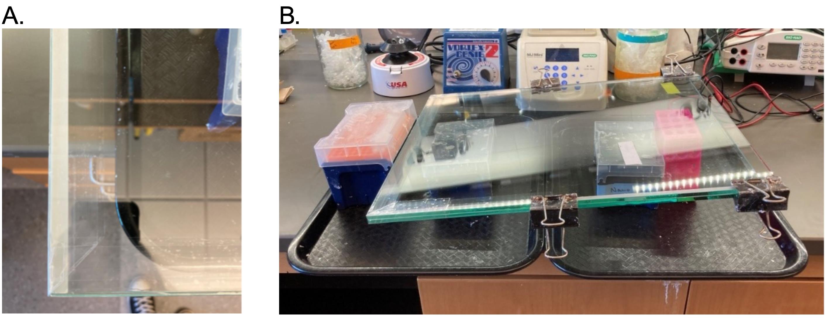
Figure 9. Taping of the gel cast and gel cast setup for gel pouring. (A) Shipping tape sealing the bottom of the gel cast (corner shown). The first layer of tape is shorter and offset to be higher on the front plate. The second layer of tape is longer and offset to be higher on the back plate. (B) Gel cast setup for gel pouring. The gel cast is balanced on a small pipette tip box on the left and a slightly taller tube rack on the right to create a gentle slope for gel pouring into the cast. Additional tip boxes provide stability.
7. Once the gel cast is set up and the gel mix is degassed, add 50 μL of TEMED and 500 μL of 10% w/v APS to the gel mix.
Critical:
1. Polymerization will begin once APS is added, so move to the next step quickly.
2. Avoid creating air bubbles in the gel mix, but also thoroughly mix the TEMED and APS throughout the gel mix before pouring. This can be done by simultaneously swirling the flask and the pipette tip.
8. Pour the gel using a 25 mL serological pipette and pipette controller.
Critical:
1. Pipet slowly to avoid overflow out of the top of the gel cast, but quickly enough to maintain the flow, and avoid bubble formation.
2. Knocking on the plates can help keep the flow even and knock out bubbles.
3. If bubbles are created, they can be moved using another gel spacer, although this can also cause more bubbles to form. The gel cast can also be stood up vertically to bring bubbles to the top, although this can cause a lot of leaking.
9. Once the gel cast is full (there will be some leftover), put in the well comb. Once the comb is in, put on more binder clips to hold the plates and comb together. Otherwise, the wells may not form cleanly.
Critical: It is important to have extra gel mix at the top of the plates before putting in the comb to avoid introducing bubbles with the comb.
10. Allow the gel to polymerize for at least 30 min. Lie flat for even gel thickness.
Pause point: Once polymerized, the gel can be stored overnight for use the next day. Wrap with damp paper towels and cling film to prevent drying and store at RT.
11. Set up polymerized gel in the Owl Aluminum-Back Sequencer Gel Rig and fill top and bottom buffer reservoirs with 1× TBE (dilute 4× TBE with ultrapure H2O).
12. Preheat polymerized gel by running at 55 W for at least 45 min.
13. Load 6 μL of each reverse transcription reaction and run the gel at 55 W.
Notes:
1. Run time depends on RNA length and what area of the RNA needs visualization. For an RNA of about 160 nucleotides, run times of 4–6 h are common.
2. Blow out the wells using a Luer-Lok syringe with a 21-gauge needle before loading. If there are many reactions to load, blow out the wells multiple times throughout loading, as such small wells fill with urea quickly, which makes sample loading more difficult.
14. Once the gel is done running, take the gel down. Check reservoirs for radioactivity with a Geiger counter before disposing of the running buffer. Pull plates apart by taking out spacers and using a razor blade to pry them apart. The gel should stick to the blank plate. Cover the gel on the blank plate with filter paper and then flip everything over so the filter paper is on the bench top (bottom to top: filter paper, gel, plate). Lift the bottom of the blank plate (the area that is Rain-X treated). The gel should stick to the filter paper. Gently pull the blank plate up from the gel + filter paper. The gel should transfer to the filter paper. Cut the gel + filter paper down to the area of interest. Cover the gel + filter paper with cling film (bottom to top: filter paper, gel, cling film).
Critical:
1. Lift the blank glass plate slowly from the gel + filter paper, as the thin gel will rip very easily.
2. Check the gel with the Geiger counter after transferring to the filter paper to ensure there is radioactivity in the expected areas.
15. Dry filter paper + gel + cling film on the gel dryer.
Note: Specifics on vacuum pressure and dry time will depend on the gel dryer. For the gel dryer listed in Equipment, 45 min at about 15 inches Hg vacuum pressure and 80 °C is sufficient.
16. While the gel is drying, clean gel glass plates, spacers, and well comb with 1% Alconox, warm water, and Kimwipes. Rinse with ultrapure H2O and spray with 70% EtOH to dry.
17. Once the gel is dry, expose to the storage phosphor screen. Ensure the screen is blank before exposure by putting on a light box for 5 min. Tape the filter paper + gel + cling film inside the storage phosphor screen cassette to keep the position stable. Dependent on the radioactivity level, overnight exposure is sufficient for imaging. Longer exposure, up to two weeks, may improve resolution.
18. Image the storage phosphor screen using the Amersham Typhoon. Use the Phosphor Imaging scanning mode. Select the scanning area corresponding to the exposed area of the screen. Set pixel size to 100 μm. Set the photo multiplier tube (PMT) to 950. Save image as a .gel file.
Notes:
1. Pixel size can be changed depending on the desired resolution.
2. PMT settings can be changed based on radioactivity level, but the screen can only be imaged once per exposure.
3. Additional file types can be saved based on preference. The recommended file type is necessary for SAFA analysis.
19. If additional exposure is not required, dispose of the filter paper + gel + cling film in radiation waste and blank storage phosphor screen by exposing to the light box for about 10 min.
Data analysis
SHAPE gels are analyzed by the Semi-Automated Footprinting Analysis (SAFA) software [25], available for free download at https://simtk.org/frs/?group_id=69. Analysis generally follows the published user’s manual, available at https://simtk.org/docman/?group_id=69. For gel image quantification, follow the steps for loading a gel image file, defining lanes, aligning the gel, loading a sequence file, choosing cleavage sites, assigning bands, and quantifying. When defining lanes, the best results are achieved when all lanes are defined manually. When choosing cleavage sites and assigning bands, the best results are achieved when all bands are assigned manually. After quantification, save the data in .txt format. For data normalization, follow the steps for visualizing and normalizing data. Remove non-data lanes and normalize to invariant residues across bands using the automated set invariant residues utility (t). Save the normalized data in .txt format. Calculate the degree of protection (DOP) by the ligand for a region of the RNA using the equation:
DOP = - ((L – N)/N)
Where L is the sum of the quantified peak areas of all bands of the region in the +ligand lane, and N is the sum of the quantified peak areas of all bands of the region in the +NMIA lane. Remember that bands in non-ddNTP lanes will be offset by one position from the ddNTP lane bands (for example, an NMIA lane band at the same horizontal position as a ddNTP band at position 5 corresponds to NMIA reactivity at RNA position 4). DOP values between different ligands can be statistically compared using unpaired t-tests, given sufficient replicates.
Part IV: Stress granule (SG) and U-body assay
Materials and reagents
Biological materials
SG assay
1. Co-transfection fluorescent protein plasmid, such as NLS-TagBFP (Addgene, catalog number: 55265), if using stable cells that express an SG marker fusion protein
2. Construct with Riboglow array that localizes to SGs, such as (1/2)NORAD-A(4×) (Addgene, catalog number: 199208) (see Section A of the Procedure) [20]
3. SG marker fusion protein plasmid, such as pEGFP-C1-G3BP1-WT (Addgene, catalog number: 135997), if transiently transfecting
4. U-2 OS cells (ATCC, catalog number: HTB-96) stably expressing an SG marker fusion protein or U-2 OS cells (ATCC, catalog number: HTB-96) to be transiently transfected with the SG marker fusion protein later
U-body assay
1. Construct with truncated Riboglow aptamer that localizes to U-bodies, such as env8-AD-5’antiPNA-U1 (Addgene, catalog number: 233011) (see Section A of the Procedure) [12]
2. U-2 OS cells (ATCC, catalog number: HTB-96)
3. U-body marker fusion protein plasmid, such as EGFP-SMN1 (Addgene, catalog number: 37057) that also acts as a co-transfection fluorescent protein plasmid
Reagents
SG assay and U-body assay
Note: Reagents only required for one of these assays (not both) are noted below.
1. D-PBS, powder, no calcium, no magnesium (Gibco, catalog number: 21600069)
2. Fetal bovine serum (FBS) (Alta Biologicals, catalog number: F-05000-DR, aliquots from different lots were used over the course of experiments)
3. FluoroBrite DMEM (Thermo Fisher Scientific, catalog number: A1896701)
4. McCoy’s 5A, powder, with L-glutamine, without sodium bicarbonate, suitable for cell culture (Sigma-Aldrich, catalog number: M4892)
5. Opti-MEM reduced serum medium, no phenol red (Invitrogen, catalog number: 11058021)
6. Penicillin-Streptomycin (P/S) (10,000 U/mL) (Invitrogen, catalog number: 15140163)
7. Riboglow probe (here, Cbl-PNA-ATTO590, generated in-house) [12]
8. Sodium bicarbonate, powder, suitable for cell culture (Sigma-Aldrich, catalog number: S5761)
9. Solvents: DMSO (Sigma-Aldrich, catalog number: 276855) and ultrapure water (from Milli-Q® Benchtop Lab Water Purification System)
10. TransIT-LT1 transfection reagent (MirusBio, catalog number: MIR 2304)
11. Trypan Blue 0.4% (Gibco, catalog number: 15250061)
12. Trypsin-EDTA 0.05% (Gibco, catalog number: 25300054)
Specific to SG assay
1. Sodium (meta)arsenite ≥90% (Sigma-Aldrich, catalog number: S7400)
Caution: Sodium arsenite is toxic. Dispose of any solutions containing sodium arsenite in hazardous chemical waste. Use appropriate PPE when handling.
Specific to U-body assay
1. NucBlue live-cell stain (Life Technologies, catalog number: R37605)
2. Thapsigargin, ≥97% (Calbiochem, catalog number: 586005)
Caution: Thapsigargin is toxic. Dispose of any solutions containing thapsigargin in hazardous chemical waste. Use appropriate PPE when handling.
Solutions
SG assay & U-body assay
Note: Solutions only required for one of these assays (not both) are noted below.
1. Cell culture media (McCoy’s 5A) (see Recipes)
2. Cell culture media without antibiotics [McCoy’s 5A (10% FBS)] (see Recipes)
3. Complete cell culture media [McCoy’s 5A (10% FBS, 1× P/S)] (see Recipes)
4. D-PBS with no Mg2+ or Ca2+ (see Recipes)
5. Imaging media [FluoroBrite DMEM (10% FBS)] (see Recipes)
6. Riboglow probe 200 μM in DMSO (see Recipes)
Specific to SG assay
1. Complete cell culture media with 0.5 mM arsenite (see Recipes)
2. Imaging media with 0.5 mM arsenite (see Recipes)
3. Riboglow probe, 5 μM in D-PBS with 2.5% DMSO (see Recipes)
4. Sodium arsenite, 50 mM (100×, see Recipes)
Specific to U-body assay
1. Complete cell culture media with thapsigargin (see Recipes)
2. Imaging media with thapsigargin (see Recipes)
3. Riboglow probe 50 μM in D-PBS with 25% DMSO (see Recipes)
4. Thapsigargin, 1 mM (100×, see Recipes)
Recipes
SG assay & U-body assay
1. Cell culture media (McCoy’s 5A)
Dissolve sodium bicarbonate powder in approximately 400 mL of McCoy’s 5A without sodium bicarbonate. Adjust pH to 7.2 with HCl and NaOH, if necessary. Bring to 500 mL with McCoy’s 5A without sodium bicarbonate. Sterilize by passing through a 0.22-μm filter into a sterile container. Store at 4 °C.
| Reagent | Final concentration | Quantity or volume |
|---|---|---|
| Sodium bicarbonate | 2.2 g/L | 1.1 g |
| McCoy’s 5A without sodium bicarbonate | n/a | Up to 500 mL |
| Total | n/a | 500 mL |
2. Cell culture media without antibiotics [McCoy’s 5A (10% FBS)]
Store at 4 °C. Prewarm to 37 °C before use.
| Reagent | Final concentration | Quantity or volume |
|---|---|---|
| McCoy’s 5A | 90% (v/v) | 45 mL |
| FBS | 10% (v/v) | 5 mL |
| Total | n/a | 50 mL |
3. Complete cell culture media [McCoy’s 5A (10% FBS, 1× P/S)]
Store at 4 °C. Prewarm to 37 °C before use.
| Reagent | Final concentration | Quantity or volume |
|---|---|---|
| McCoy’s 5A | 89% (v/v) | 445 mL |
| FBS | 10% (v/v) | 50 mL |
| P/S (10,000 U/mL) | 1% (v/v), 100 U/mL | 5 mL |
| Total | n/a | 500 mL |
4. D-PBS with no Mg2+ or Ca2+
Dissolve D-PBS powder in approximately 400 mL of ultrapure H2O. Adjust pH to 7.2 with HCl and NaOH, if necessary. Bring to 500 mL with ultrapure H2O. Sterilize by passing through a 0.22 μm filter into a sterile container. Store at room temperature. Do not warm before washing cells.
| Reagent | Final concentration | Quantity or volume |
|---|---|---|
| D-PBS | 1× | 4.775 g |
| Ultrapure H2O | n/a | Up to 500 mL |
| Total | n/a | 500 mL |
5. Imaging media [FluoroBrite DMEM (10% FBS)]
Store at 4 °C. Prewarm to 37 °C before use.
| Reagent | Final concentration | Quantity or volume |
|---|---|---|
| FluoroBrite DMEM | 90% (v/v) | 45 mL |
| FBS | 10% (v/v) | 5 mL |
| Total | n/a | 50 mL |
6. Riboglow probe 200 μM in DMSO
Store all Cbl probes in dry DMSO at -20 °C. The probe stock solution can be frozen and thawed multiple times without a loss in quality. Overall, the ATTO590 probes remain stable for an extended period (>12 months) when stored in dry DMSO at -20 °C and protected from prolonged light exposure. ATTO488 probes are sensitive to freeze-thaw cycles or storage for long periods of time; use within a few weeks of dissolution in DMSO.
| Reagent | Final concentration | Quantity or volume |
|---|---|---|
| Riboglow probe 400 μM in DMSO | 200 μM | 25 μL |
| DMSO | n/a | 25 μL |
| Total | n/a | 50 μL |
Specific to SG assay
1. Complete cell culture media with 0.5 mM sodium arsenite
Make 2 mL/35 mm dish fresh each day for imaging. Prewarm to 37 °C before use.
| Reagent | Final concentration | Quantity or volume |
| McCoy’s 5A (10% FBS, 1× P/S) | 99% (v/v) | 1.98 mL |
| Sodium arsenite 50 mM (100×) | 1% (v/v), 1×, 0.5 mM | 20 μL |
| Total | n/a | 2 mL |
2. Imaging media with 0.5 mM sodium arsenite
Make 2 mL/35 mm dish fresh each day for imaging. Prewarm to 37 °C before use.
| Reagent | Final concentration | Quantity or volume |
|---|---|---|
| FluoroBrite DMEM (10% FBS) | 99% (v/v) | 1.98 mL |
| Sodium arsenite 50 mM (100×) | 1% (v/v), 1×, 0.5 mM | 20 μL |
| Total | n/a | 2 mL |
3. Riboglow probe 5 μM in D-PBS with 2.5% DMSO
Store in aluminum foil during use. Riboglow probes are less stable in aqueous solutions, so do not keep after its first day of use and do not freeze-thaw.
| Reagent | Final concentration | Quantity or volume |
|---|---|---|
| Riboglow probe 200 μM in DMSO | 5 μM | 1 μL |
| D-PBS | n/a | 39 μL |
| Total | n/a | 40 μL |
4. Sodium arsenite 50 mM (100×)
Dissolve sodium (meta)arsenite in approximately 40 mL of ultrapure H2O. Bring up to 50 mL with ultrapure H2O. Aliquot into single-use tubes. Store at -20 °C (recommended near the back of the freezer to avoid freeze-thaw cycles). Aliquots that have not undergone freeze-thaw cycles are good for at least one year. Thaw just before use.
| Reagent | Final concentration | Quantity or volume |
|---|---|---|
| Sodium (meta)arsenite | 50 mM (100×) | 0.325 g |
| Autoclaved ultrapure H2O | n/a | Up to 50 mL |
| Total | n/a | 50 mL |
Specific to U-body assay
1. Complete cell culture media with 10 μM thapsigargin
Make 2 mL/35 mm dish fresh each day for imaging. Prewarm to 37 °C before use.
| Reagent | Final concentration | Quantity or volume |
|---|---|---|
| McCoy’s 5A (10% FBS, 1% P/S) | 99% (v/v) | 1.98 mL |
| Thapsigargin 1 mM (100×) | 1% (v/v), 1×, 10 μM | 20 μL |
| Total | n/a | 2 mL |
2. Imaging media with 10 μM thapsigargin
Make 2 mL/35 mm dish fresh each day for imaging. Prewarm to 37 °C before use.
| Reagent | Final concentration | Quantity or volume |
|---|---|---|
| FluoroBrite DMEM (10% FBS) | 99% (v/v) | 1.98 mL |
| Thapsigargin 1 mM (100×) | 1% (v/v), 1×, 10 μM | 20 μL |
| Total | n/a | 2 mL |
3. Riboglow probe 50 μM in D-PBS with 25% DMSO
Store in aluminum foil during use. Riboglow probes are less stable in aqueous solutions, so do not keep after its first day of use and do not freeze-thaw.
| Reagent | Final concentration | Quantity or volume |
|---|---|---|
| Riboglow probe 200 μM in DMSO | 50 μM | 1 μL |
| D-PBS | n/a | 3 μL |
| Total | n/a | 4 μL |
4. Thapsigargin 1 mM (100×)
Aliquot into single-use tubes. Store at -20 °C (recommended near the back of the freezer to avoid freeze-thaw cycles). Aliquots that have not undergone freeze-thaw cycles are good for at least one year. Thaw just before use.
| Reagent | Final concentration | Quantity or volume |
|---|---|---|
| Thapsigargin | 1 mM (100×) | 0.0325 g |
| Autoclaved ultrapure water | n/a | Up to 50 mL |
| Total | n/a | 50 mL |
Laboratory supplies
SG assay & U-body assay
1. Aspirating pipettes (Falcon, catalog number: 357558)
2. CellStar cell culture dishes, 10 cm (Grenier, catalog number: P7612) or other tissue culture–treated dishes (any reputable vendor)
3. Conical tubes 15 mL (VWR, catalog number: 89039-664)
4. Conical tubes 50 mL (VWR, catalog number: 89039-656)
5. Countess cell counting chamber slides (Invitrogen, catalog number: C10283), if using a Countess automatic cell counter
6. DRIERITE desiccant (DRIERITE, catalog number: 21001)
7. Glass-bottom cell culture dishes 35 mm #1.5 (Ibidi, catalog number: 81218-200) or homemade imaging dishes (described below in Procedure)
a. Glass coverslip 18×18 mm square #1.5 (VWR, catalog number: 16004-326)
b. SYLGARD 184 Silicone Elastomer Kit (Dow, catalog number: 4019862)
c. TC-treated cell culture dishes, 35 mm (Corning, catalog number: 430165)
8. Glass beads ≤106 μm, acid-washed (Sigma-Aldrich, catalog number: G4649)
9. Microcentrifuge tubes 1.5 mL (VWR, catalog number: 20170-038)
10. Microcentrifuge tubes 0.6 mL (VWR, catalog number: 76332-062)
11. Nylon screen, 100 mesh, 3 in. × 3 in. (Ted Pella, Inc., catalog number: 41-3110)
12. pH indicator paper that spans ~pH 7 (any reputable vendor)
13. Serological pipettes: 5 mL (Fisherbrand, catalog number: 13-678-11D), 10 mL (Fisherbrand, catalog number: 13-678-11E), 25 mL (Fisherbrand, catalog number: 13-678-11)
14. Stainless steel laboratory spatula for weighing solid reagents (any reputable vendor)
15. Sterile, filtered, low-retention pipette tips: 1,000 μL (VWR, catalog number: 76322-154), 200 μL (VWR, catalog number: 76322-150), 20 μL (VWR, catalog number: 76322-134), 10 μL (VWR, catalog number: 76322-528), and 2 μL (VWR, catalog number: 76327-214)
16. Tape (any reputable vendor), if making homemade imaging dishes
17. Weighing paper (Fisher Scientific, catalog number: 09-898-12A)
Equipment
SG assay & U-body assay
1. Set of adjustable micropipettes covering a range of 0.1–1,000 μL (e.g., 0.1–2 μL, 2–20 μL, 20–200 μL, 100–1,000 μL)
2. Analytical balance (Denver Instrument, catalog number: TB-224)
3. Biosafety cabinet (any reputable vendor)
4. Centrifuge with swinging bucket for 15–50 mL conical tubes (Beckman, model: GPR Centrifuge, catalog number: 349702)
5. Confocal microscope with high NA objective and appropriate laser lines
a. Nikon Ti-E A1R laser scanning confocal microscope
b. 100× (1.45 NA) Plan Apo Lambda oil objective (Nikon)
c. 405-nm (Coherent OBIS), 488-nm (Coherent OBIS), 561-nm (Coherent Sapphire), and 640-nm (Coherent OBIS) lasers
d. PMT detectors for 405-nm and 488-nm lasers (Nikon), GaAsp PMT for 561-nm and 640-nm lasers (Nikon)
e. Immersion oil Type F (Nikon)
6. Constructed beadloader (described below in Procedure)
7. Countess II automatic cell counter (Life Technologies); not sold by the vendor anymore, upgraded to Countess III Automatic Cell Counter (Invitrogen). Alternatively, use a hemocytometer (any reputable vendor) and manually count cells under a simple microscope with a 10× objective and phase contrast
8. Incubator 37 °C and 5% CO2 (Heracell VIOS 160i CO2 Incubator, Thermo Scientific, catalog number: 51033556)
9. Industrial bench punch (Roper Whitney, catalog number: 131020160) and Type O Round Punch Size 3/8 in. (Roper Whitney, catalog number: 300160375), if making homemade imaging dishes
10. Large plastic bin with a good seal, if making homemade imaging dishes, to keep them sterile outside of the biosafety cabinet (any reputable vendor)
11. Pipet-Aid XP (Drummond Scientific, catalog number: 4-000-101)
12. Shaker (any reputable vendor)
13. Simple microscope with 4× or 10× magnification and phase contrast (any reputable vendor)
14. Small plastic or glass bin with a good seal, to store the beadloader (any reputable vendor)
15. UV sterilization lamp (Cole Parmer, 97505 30 Watts)
16. Vacuum pump and plastic tubing (to be used with aspirating pipettes; GAS, DOA-P704-AA or any reputable vendor)
17. Vortex mixer (Fisher Scientific, catalog number: 02215370)
18. Water bath set to 37 °C (Fisher Scientific, model: Isotemp 120, catalog number: 15-460-20)
Software and datasets
SG assay & U-body assay
1. Fiji (ImageJ2 with common plugins) (ImageJ, Version 2.9.0); we have noted no issues with versions slightly older or slightly newer than this. Used for manually analyzing images. This software is open source and can be downloaded at https://imagej.net/software/fiji/downloads.
2. GraphPad Prism [version 10.3.0 (507) released July 30, 2024; GraphPad Software, San Diego, CA]. Used for data plotting and statistics. This is commercial software and requires a paid license. Free alternatives include SciDAVis or LabPlot.
3. Microsoft Excel [version 16.97.2 (25052611); released May 27, 2025; Microsoft 365]. Used for organizing manually collected data and calculations. This is commercial software and requires a paid license. Free alternatives include Google Sheets.
Procedure
The SG and U-body assays have been divided into three main steps: Preparing the Riboglow-tagged constructs (Figure 10A), preparing imaging dishes and the beadloader (Figure 10B), and preparing the cells for imaging and the imaging process (Figure 10C). This procedure follows portions of other published protocols, but it is published in its entirety here, for convenience [10,12,17,26].
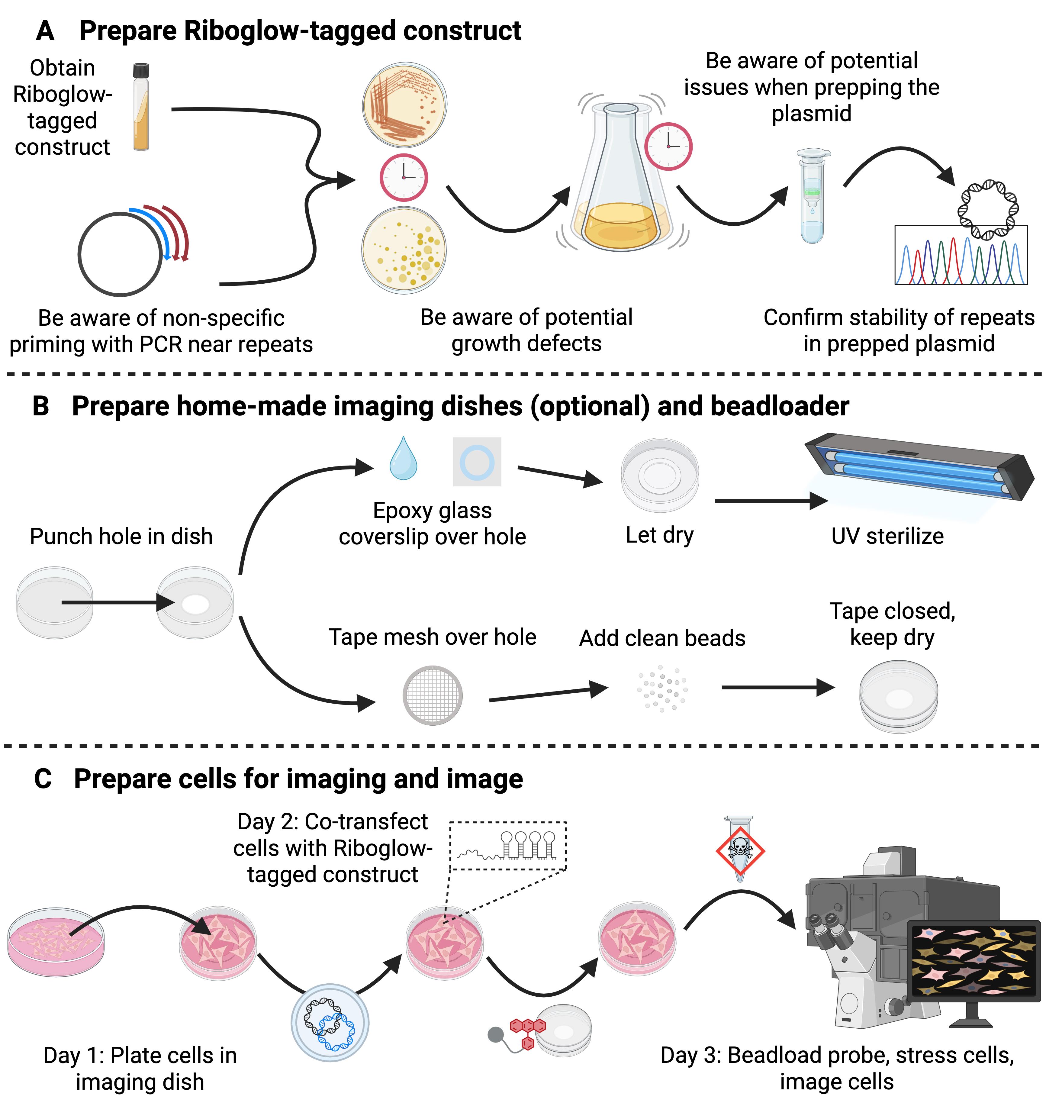
Figure 10. General roadmap for the SG assay and the U-body assay. (A, B) Equipment and preparation steps to complete before the SG or U-body assays. (C) Preparation of cells for imaging, imaging, and image analysis.
In the SG and U-body assays, the protocol is written specifically for the cell line, SG or U-body marker fusion fluorescent proteins, co-transfection markers, Riboglow-tagged RNAs, Riboglow probe and probe concentrations, and stressor concentrations that were used in [12]. However, this protocol is versatile, and many pieces can be exchanged for others if desired. For example, the Riboglow probe and all fluorescent proteins used as SG or U-body marker proteins, or co-transfection markers, can be exchanged to suit the imaging needs. Ensure that the pieces in the new regime contain non-overlapping fluorescence excitation and emission spectra. The RNA of interest used in either assay can also be exchanged by molecular cloning to answer a specific research question. However, in the SG assay, when comparing conditions with the same RNA-of-interest (e.g., different probes, different RNA tags, and different stressors), we strongly recommend using the (1/2)NORAD-4xenv8-3’antiPNA construct with the Cbl-PNA-ATTO590 probe, because this combination significantly increases the dynamic range of the assay [12]. Finally, we advise that the Riboglow probes are beadloaded into cells, since they are not cell-permeable. Beadloading allows for the introduction of the probe into many adherent cells in a dish at one time. Finally, this protocol can also be easily adapted to other RNA-imaging systems, like the MS2-MCP system, by exchanging the Riboglow array for the other tool.
Critical: Steps or notes only required for one of the SG or U-body assays (not both) are noted below.
A. Preparing Riboglow-tagged constructs
Specific for SG assay
Cloning a construct with a Riboglow array:
In lieu of providing an extensive protocol with steps to clone a construct with a Riboglow array (a construct with multiple Riboglow aptamers linked in series), we provide general cloning advice:
1. We have had success with both restriction digest/ligation and Gibson methods when creating constructs with a Riboglow array; however, we recommend restriction digest/ligation methods when altering a piece near the Riboglow array. The repetitive nature of the Riboglow array may make designing specific primers for PCR products near the array difficult and make Gibson cloning more laborious.
2. Because designing specific primers near the edges of the Riboglow array is difficult, we recommend using whole plasmid nanopore sequencing to confirm the desired sequence.
3. After obtaining a positive clone, we recommend transforming your construct into special recombinase-deficient chemically competent E. coli cell lines intended for repetitive sequences, such as NEB Stable (NEB, C3040), before larger-scale preparation or creating glycerol stocks intended for longer-term storage. For each successive preparation of the DNA, we recommend sequencing the plasmid to ensure fidelity.
4. We have noticed growth defects in the (1/2)NORAD construct. When altering this construct, positive clones often do not show up until after an overnight incubation step at 37 °C and an additional day/overnight incubation at room temperature. The colonies containing the (1/2)NORAD construct are also often much smaller than the incorrect colonies that appear after the initial 37 °C overnight incubation. We think this may be due to potential leaky expression of constructs following the CMV promoter in bacteria, but we have no concrete evidence of this yet.
Preparing plasmid DNA of a construct with a Riboglow array:
In lieu of providing an extensive protocol with steps to prepare a DNA plasmid of a construct containing a Riboglow array, we provide general advice to consider while following manufacturer instructions from your chosen DNA plasmid miniprep or midiprep kit:
1. When growing constructs with a Riboglow array, and especially when growing a (1/2)NORAD construct, treat the construct as a low-copy plasmid. Larger cultures for DNA preparation, started from a colony on an agar plate, sometimes result in a bacterial culture with a stringy appearance. To avoid this, we recommend inoculating a small culture and allowing it to grow in a 37 °C shaker-incubator for 4–8 h. Then, inoculate the larger culture with some of the small culture and grow overnight in a 37 °C shaker-incubator for DNA preparation.
2. We have noticed that some constructs with either (1/2)NORAD or a Riboglow array do not consistently midiprep well. Sometimes a construct will prep well, and sometimes it will not. We have not been able to determine what aspects allow them to prep well. In these cases, they have been amenable to miniprep-scale DNA plasmid preparation every time in our hands.
Specific for U-body assay
Cloning a construct with a truncated Riboglow aptamer
In lieu of providing an extensive protocol with steps to clone a construct with a truncated Riboglow aptamer, we provide general cloning advice:
1. We have had success with both restriction digest/ligation and Gibson methods when creating constructs with a Riboglow aptamer; however, we recommend Gibson cloning, when possible, due to its decreased number of background colonies compared to restriction digest/ligation cloning, especially when splitting the vector at the antibiotic resistance gene and DpnI digesting any plasmid that was used as a PCR template.
2. After obtaining a positive clone, it is not necessary to transform your construct into a special recombinase-deficient E. coli competent cell line, as it is for constructs with a longer Riboglow array.
3. We have not noticed any growth defects with the U1 constructs or with constructs containing a single Riboglow aptamer.
Preparing plasmid DNA of a construct with a truncated Riboglow aptamer:
In lieu of providing an extensive protocol with steps to prepare a DNA plasmid of a construct containing a truncated Riboglow aptamer, we provide general advice to consider while following manufacturer instructions from your chosen DNA plasmid miniprep or midiprep kit:
1. When growing constructs with a truncated Riboglow aptamer, treat the construct as a high-copy plasmid unless the plasmid backbone is normally grown as a low-copy plasmid.
2. We have not noticed any issues while midiprepping U1 constructs or constructs containing a single Riboglow aptamer.
B. Making homemade imaging dishes (optional)
1. Remove the lid from 35 mm tissue culture–treated cell culture dishes. Use an industrial hole punch to punch a 3/8 in. hole in the middle of the dish.
2. Mix silicone elastomer according to the manufacturer’s instructions and use a small amount to adhere 18 mm × 18 mm square glass coverslips onto the bottom of the dish.
3. Let the silicone elastomer cure according to the manufacturer’s instructions.
4. In a biosafety cabinet, sterilize both the lids and the bottom of the dishes with a UV lamp for 15 min. Flip the lids and the bottoms of the dishes over. Sterilize again with a UV lamp for 15 min. Combine the lids and bottoms in a sterile plastic bin with a tight-sealing lid before removing everything from the biosafety cabinet to keep the imaging dishes sterile for future use.
C. Making a homemade beadloader
1. Pour approximately 5 mL of acid-washed ≤106 mm glass beads into a 50 mL conical tube. Pour approximately 25 mL of 2 M NaOH into the same conical tube. Mix gently for 2 h with a shaker or rotator.
2. Decant the NaOH solution from the beads. If necessary, spin down the beads by centrifuging at ~1,000× g for 1 min.
3. Rinse the beads with ultrapure water until the water eluent is a neutral pH. Decant the water each time, centrifuging if necessary.
4. Rinse the beads 2–3× with 100% EtOH. Decant the EtOH each time, centrifuging if necessary.
5. In a biosafety cabinet, spread the beads in a thin layer in a 10 cm tissue culture–treated dish. Let dry with the lid off the dish overnight or longer.
6. Sterilize the beads with a UV lamp for 15 min.
7. Make a hole in the bottom of a 35 mm dish. We use an industrial hole punch to make a 3/8 in. hole in the middle of the dish. Tape a small piece of Nylon 100 mesh over the hole.
8. Pour UV-sterilized dry glass beads into the 35 mm dish with the mesh. Keep the remainder of the beads in a tightly sealed container, e.g., a 15 mL conical. Tape the dish’s lid onto the dish to create the beadloader. Use an extra 35 mm dish lid to cover the mesh-covered hole in the beadloader during storage.
Note: After much use, the beadloader can be easily disassembled, and more UV-sterilized dry glass beads can be added before taping the beadloader closed again.
9. Store the beadloader in a small sterile container with desiccant.
D. Preparing cells for imaging
For the timing of each step in the SG assay, see Figure 11. For the timing of each step in the U-body assay, see Figure 12.
Caution: The steps for preparation of the cell line for imaging should be performed in a biosafety cabinet with appropriate PPE. The complete cell culture media includes penicillin/streptomycin; however, every precaution should be taken to ensure that the cells remain sterile during preparation and to protect yourself from potential hazards. 70% EtOH should be used to sterilize items going into and coming out of the biosafety cabinet.
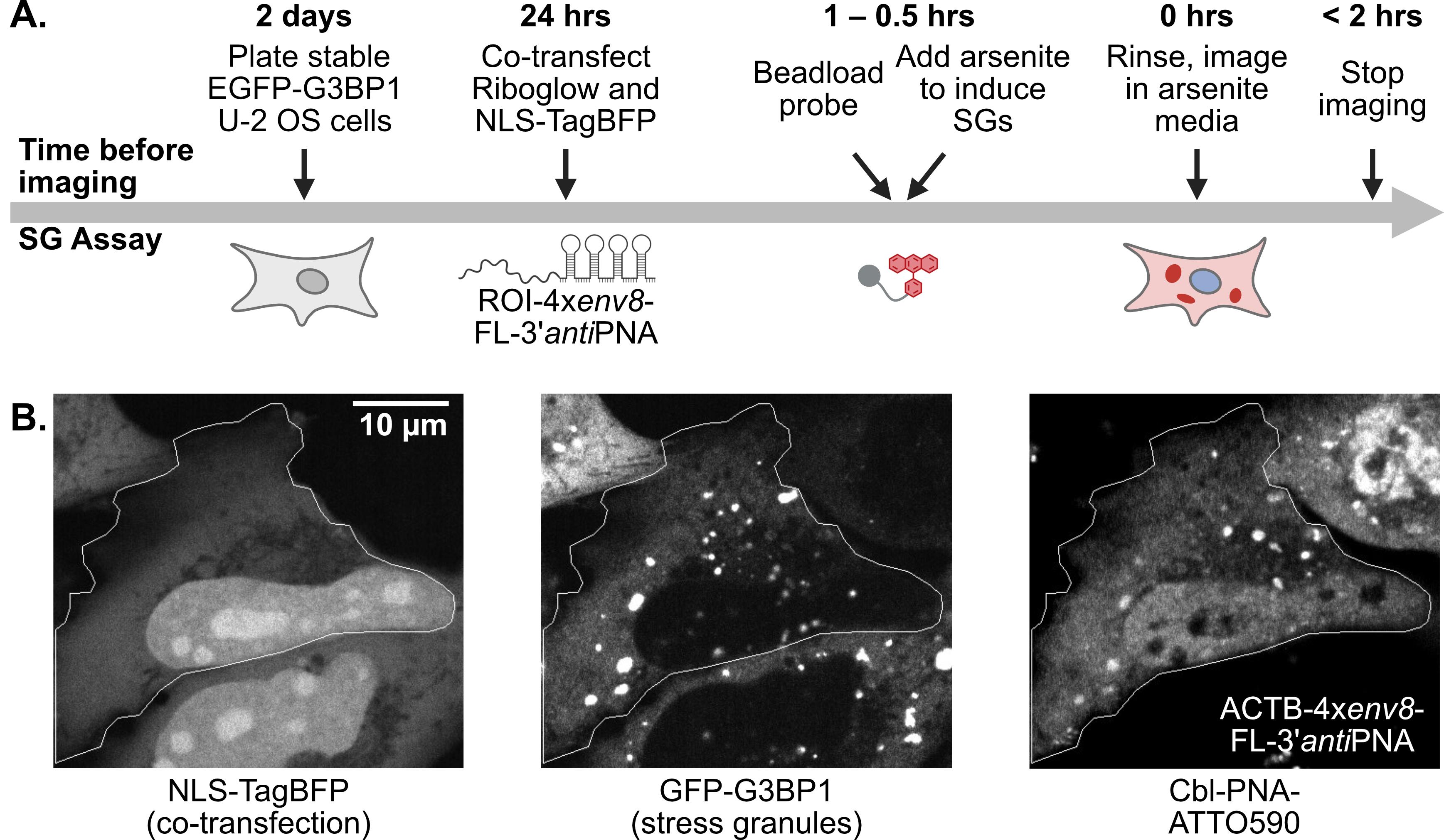
Figure 11. Timing of SG assay. (A) Schematic of the timeline of the SG assay. (B) Example images from the SG assay in U-2 OS cells stably expressing EGFP-G3BP1 co-transfected with NLS-TagBFP and ACTB-4xenv8-FL-3’antiPNA and beadloaded with 5 μM Cbl-PNA-ATTO590. Cell outline in white. Scale bar = 10 μm.
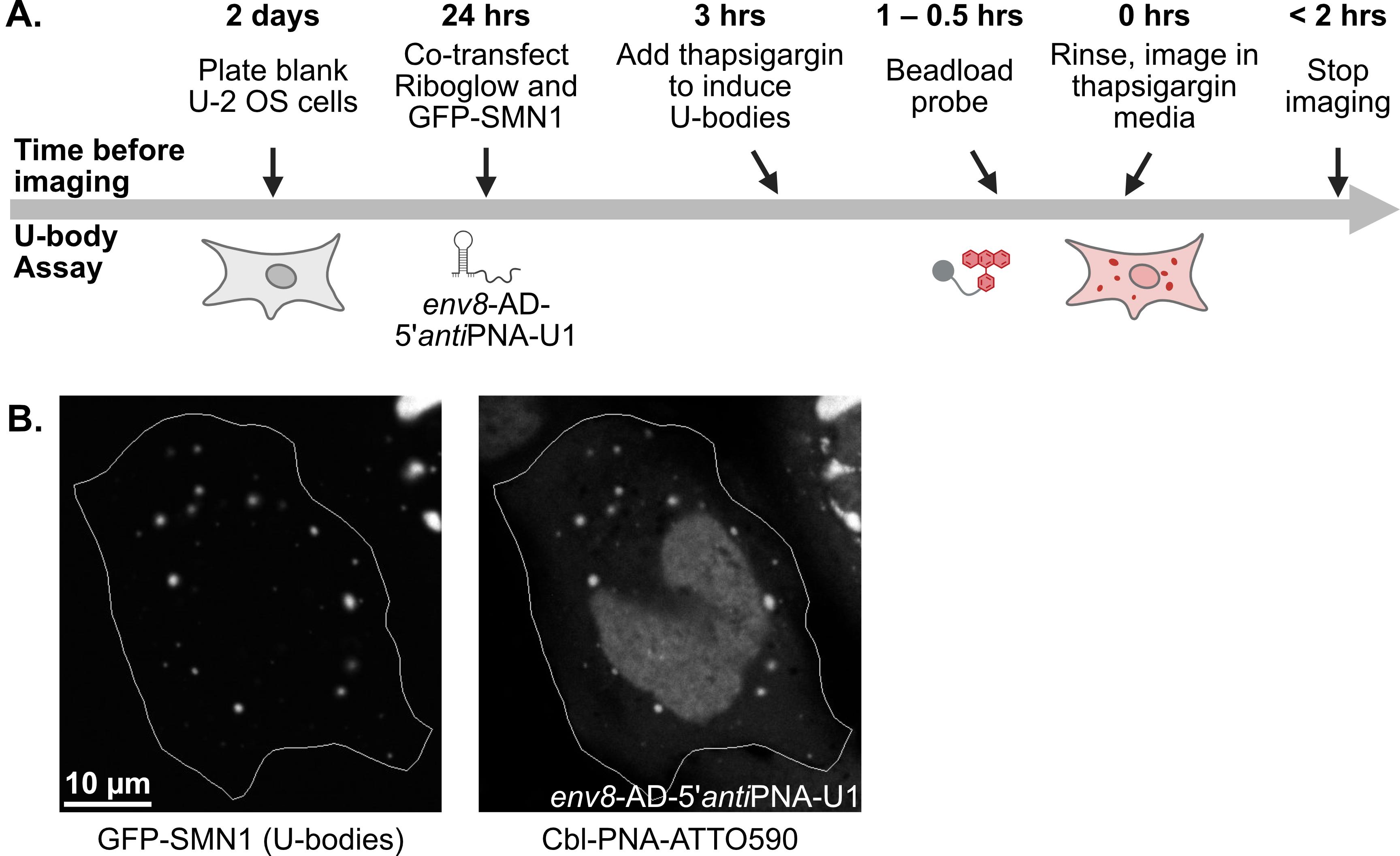
Figure 12. Timing of U-body assay. (A) Schematic of the timeline of the U-body assay. (B) Example images from the U-body assay in U-2 OS cells co-transfected with GFP-SMN1 and env8-AD-5’antiPNA-U1 and beadloaded with 50 μM Cbl-PNA-ATTO590. Cell outline in white. Scale bar = 10 μm.
Day 1 (plating cells into imaging dishes):
1. Prewarm complete cell culture media and trypsin at 37 °C in a water bath.
2. Passage cells as normal, saving approximately 2 million cells for a continuation 10 cm dish.
3. Plate 175,000–185,000 cells into each 35 mm imaging dish, adding prewarmed complete cell culture media up to 2 mL for each dish.
4. Incubate cells at 37 °C and 5% CO2.
Day 2 (transfecting cells with your construct and a co-transfection marker):
1. Plan such that transfection will occur approximately 24 h before imaging. Prewarm complete cell culture media without antibiotics at 37 °C in a water bath. Prewarm TransIT-LT1 and Opti-MEM to room temperature. Thaw plasmid DNA if necessary.
Critical for the SG assay: Transfection for longer than 30 h significantly decreased the dynamic range between a negative control and cells transfected with a Riboglow-tagged construct.
2. Use a simple microscope with a 4× or 10× objective and phase contrast to check the confluency of your cells.
3. SG assay: Combine equimolar amounts (~292 fmol) of your Riboglow-tagged construct plasmid and a co-transfection fluorescent protein plasmid, such as NLS-TagBFP, in a 0.6 mL tube. Mix by pipetting. Prepare the transfection mixtures for each dish separately.
U-body assay: Combine ~448 fmol of the Riboglow-tagged construct plasmid and ~65 fmol of the U-body marker fusion protein plasmid, such as EGFP-SMN1 (which also acts as a co-transfection fluorescent protein plasmid) in a 0.6 mL tube. Mix by pipetting. Prepare the transfection mixtures for each dish separately.
Note for both assays: Co-transfection amounts are based on reference [10], from data shown in Supplemental Figure 17. Co-transfection of 1 μg of NLS-TagBFP (~292 fmol) and 1 μg of mNG-A(1×) results in cells expressing both plasmids 94% of the time. We do not recommend decreasing the molar ratio of construct plasmid:co-transfection plasmid, but you can increase it to ensure that an even higher percentage of cells with the co-transfection plasmid express the construct.
4. Add 100 μL of Opti-MEM to each tube. Mix by pipetting.
5. Add TransIT-LT1 at a ratio of 3 μL of TransIT-LT1 to 1 μg of total DNA to each tube. Pipette five times to mix.
Note: While this ratio provides sufficient transfection efficiencies for this assay, we have not done extensive optimization of this ratio.
6. Incubate the transfection mix at room temperature for 20 min.
7. Aspirate media from cells. Add 2 mL of fresh prewarmed cell culture media without antibiotics to each dish.
8. Add the transfection mixture dropwise on top of the media (holding the pipette above the media, not pipetting into the media).
9. Incubate cells at 37 °C and 5% CO2.
Specific to SG assay
Day 3 (beadloading cells and treating with arsenite):
1. Prewarm complete cell culture media and imaging media to 37 °C in a water bath. Thaw an aliquot of 50 mM (100×) sodium arsenite and an aliquot of 200 μM (40×) Riboglow probe.
2. Freshly prepare complete cell culture media with 0.5 mM arsenite, imaging media with 0.5 mM arsenite, and 5 μM Riboglow probe according to the recipes above.
Note: We could detect a higher enrichment of the Cbl-PNA-ATTO590 probe in SGs in cells expressing a Riboglow-tagged construct when beadloading 10× less probe (0.5 μM); however, we would not recommend this lower probe concentration for the first-generation probes Cbl-4xGly-ATTO590 or Cbl-5xPEG-ATTO590 [12].
3. From 30 min to 1 h before imaging, aspirate media from cells. Pipette 3 μL of 5 μM Riboglow probe onto the cells in the center of the dish. Uncap the beadloader and tap it above the imaging dish of cells to add a single layer of beads. Tap on more beads if necessary. See Video 1.
Note: Lifting and tilting the dish will allow you to see the beads easily.

4. Tap the dish of cells with the probe and beads onto the hood of the biosafety cabinet 7–8×.
Note: We recommend practicing the force necessary for beadloading before performing a full imaging experiment. When we mimic the force that we used in these experiments while tapping the dish on an ordinary lab scale, the scale read ~30–70 g.
5. Carefully add 2 mL of prewarmed complete cell culture media with 0.5 mM arsenite to the dish, pipetting the media into the side of the dish instead of directly on top of the desired cells.
6. Incubate cells at 37 °C and 5% CO2 for 30 min to 1 h.
Critical for SG assay: The rate of SG formation depends on temperature and CO2. Incubating the cells at 37 °C and 5% CO2 ensures that most cells will form SGs during this incubation period before imaging.
Note: At this time, also turn on the microscope and environmental chamber to 37 °C, 5% CO2, and >80% humidity (step 1 in Imaging).
7. Remove the lid from the dish of cells and set it on the hood of the biosafety cabinet. Prop the dish of cells on top of the lid so that the dish is at a slant. Remove the arsenite media from the cells and put it into hazardous chemical waste. See Video 2.
Note: Due to their small size, glass beads are not saved for cleaning and re-use.
8. Rinse the cells 1× with 1 mL of prewarmed imaging media with 0.5 mM arsenite. With a 1,000 μL micropipette, remove the rinse and put it into hazardous chemical waste.
Note: Angling the dish helps in this process.
9. Add a final 1 mL of prewarmed imaging media with 0.5 mM arsenite to the dish. Put the lid back on the dish before moving to imaging.
Critical: Stagger this beadloading process so that cells are in arsenite media for approximately 30 min to 1 h and are beadloaded for approximately 30 min to 3.5 h. After approximately 45 min to 1 h in 0.5 mM arsenite media, most cells have large SGs that are easy to analyze. After approximately 2.5 h in 0.5 mM arsenite media, cells begin to die and are unanalyzable.
Specific to U-body assay
Day 3 (beadloading cells and treating with thapsigargin):
1. Prewarm complete cell culture media and imaging media to 37 °C in a water bath. Thaw an aliquot of 1 mM (100×) thapsigargin and an aliquot of 200 μM (4×) Riboglow probe.
2. Freshly prepare complete cell culture media with 10 μM thapsigargin, imaging media with 10 μM thapsigargin, and 50 μM Riboglow probe according to the recipes above.
3. Three hours before imaging, aspirate media from cells. Add 1 mL of prewarmed complete cell culture media with 10 μM thapsigargin.
4. Incubate cells at 37 °C and 5% CO2.
5. From 30 min to 1 h before imaging, remove media from cells and put it into hazardous chemical waste. Add 3 μL of 50 μM Riboglow probe onto the cells in the center of the dish. Uncap the beadloader and tap it above the imaging dish of cells to add a single layer of beads. Tap on more beads if necessary. See Video 1.
Note: Lifting and tilting the dish will allow you to see the beads easily.
6. Tap the dish of cells with probe and beads onto the hood of the biosafety cabinet 7–8×.
Note: We recommend practicing the force necessary for beadloading before performing a full imaging experiment. When we mimic the force that we used in these experiments while tapping the dish on an ordinary lab scale, the scale read ~30–70 g.
7. Carefully add 1 mL of prewarmed complete cell culture media with 10 μM thapsigargin to the dish, pipetting the media into the side of the dish instead of directly on top of the desired cells.
8. Add 1–2 drops of NucBlue live cell stain to the dish to stain the nucleus (not included in Video 1).
9. Incubate cells at 37 °C and 5% CO2 for 30 min to 1 h.
Note: At this time, also turn on the microscope and environmental chamber to 37 °C, 5% CO2, and >80% humidity (step 1 in Imaging).
10. Remove the lid from the dish of cells and set it on the hood of the biosafety cabinet. Prop the dish of cells on top of the lid so that the dish is at a slant. Remove the thapsigargin media from the cells and put it into hazardous chemical waste. See Video 2.
Note: Due to their small size, glass beads are not saved for cleaning and re-use.
11. Rinse the cells 1× with 1 mL of prewarmed imaging media with 10 μM thapsigargin. Remove the rinse and put it into hazardous chemical waste.
Note: Angling the dish helps in this process.
12. Add a final 1 mL of prewarmed imaging media with 10 μM thapsigargin to the dish. Put the lid back on the dish before moving to imaging.
Critical: Stagger this beadloading process so that cells are in thapsigargin media for approximately 3 h and are beadloaded for approximately 30 min to 3.5 h. After approximately 3 h in 10 μM thapsigargin media, most cells have U-bodies with sharp edges that are easy to analyze. After too long in 10 μM thapsigargin media, cells begin to die and are unanalyzable.
E. Imaging
Specific to SG assay
Day 3 (imaging cells):
In the accompanying paper, we collected images on a Nikon Ti-E A1R laser scanning confocal microscope with a 100× (1.45 NA) Plan Apo Lambda oil objective (Nikon) and 405-nm (Coherent OBIS), 488-nm (Coherent OBIS), 561-nm (Coherent Sapphire), and 640-nm (Coherent OBIS) lasers. The signal from excitation with 405-nm and 488-nm lasers was collected with Nikon PMT detectors, and the signal from excitation with 561-nm and 640-nm lasers was collected with GaAsp PMT detectors [12]. However, other confocal microscopes with a high NA objective should work for this assay.
1. Thirty minutes before imaging, turn on the microscope and the environmental chamber to 37 °C, 5% CO2, and >80% humidity.
Critical: The rate of SG formation depends on temperature and CO2. Incubating the cells at 37 °C and 5% CO2 ensures that most cells will continue to have SGs during imaging.
Note: Allowing a drop of oil to warm on the objective during this period will help to avoid drift during later imaging.
2. When the cells are ready to be imaged, gently place the dish of cells in the stage insert. Align the 100× oil objective (with a drop of oil) to the center of the imaging area. Lower the stage of the microscope until the oil squishes against the glass. Use Perfect Focus and slowly lower the stage until Perfect Focus engages at the approximate focal plane.
Critical: Using a lower magnification/lower NA objective, such as a 20× air (0.75 NA) objective, resulted in significantly decreased dynamic range between a negative control and cells transfected with a Riboglow-tagged construct.
3. Begin imaging in the channel expected to have signal in most cells. Locate a cell, increasing the pinhole size to the maximum value if necessary to aid in finding a fluorescent cell. Use the Perfect Focus Wheel to further refine the stage height.
4. To quickly find cells that contain all necessary components, create a new optical configuration (OC) for scanning the dish (potentially by right-clicking and duplicating a pre-made OC): only select the channels with expected signal (e.g., 405 nm, 488 nm, 561 nm). Make sure Perfect Focus is engaged in the OC. Use the resonant scanner with 2× averaging and a 2.0 AU pinhole to allow for quick scanning and the ability to keep cells in focus across a large scan area (especially important for homemade imaging dishes that are not perfectly level) while retaining sufficient image quality. Use the Scan Large Image function and this new OC to image a wide area (e.g., 9 × 9). Review the resultant image and find cells that are co-transfected with the co-transfection fluorescent protein, beadloaded with Riboglow probe, expressing the SG marker fusion protein, and that have visible SGs in the cytosol. On cells with all the necessary criteria, right-click on the cell and select Move point to center to move the stage to that cell.
5. Begin imaging in the SG marker fusion protein channel and use the Perfect Focus Wheel to focus on the SGs in the cytosol. The edges of most of the SGs should be sharp when focused properly.
Note: Over time, the edges of SGs will often become sharper. The sharp edges of the SG make analysis easier. If you would like to wait to image this cell, you can mark this point on the dish in the Multi-Point Acquisition window.
6. To image this cell, create a new OC (or adjust a pre-made OC): Only select the channels with expected signal (e.g., 405 nm, 488 nm, 561 nm). Adjust the laser powers, gain, pinhole, and dwell time to the specifications in Table 4. Image the cell with Nyquist sampling for the best image.
Note: These imaging settings are what we used, but we did not perform significant optimization before continuing with these settings. Change the settings to whatever works best for your microscope and samples. We recommend keeping a small pinhole to remove out-of-focus light and choosing a laser power and gain that do not lead to saturation of the detector in the Riboglow probe channel. Sharp edges make image analysis easier, and SGs that have saturated the detector in the Riboglow probe channel cannot be included in the analysis.
Critical:
1. If you wish to compare SG enrichment ratios across images, the settings used to collect the Riboglow probe channel must be the same across images. The settings used to collect the channels for the co-transfection of fluorescent protein and SG marker fusion protein can be changed when necessary to avoid saturation of the detector.
2. Images that were taken with a lower magnification/lower NA objective, such as a 20× air (0.75 NA) objective, gave significantly less dynamic range between a negative control with probe only and cells expressing constructs with Riboglow arrays. Images that were taken in a z-stack and then maximum intensity projected into a single image before analysis gave significantly less dynamic range between a negative control with probe only and cells expressing constructs with Riboglow arrays.
7. Repeat this process for more cells in the dish and for more imaging dishes. When done with the imaging dishes, dispose of the arsenite media in hazardous chemical waste.
Table 4. Imaging settings for SG assay
| Experiment | Imaging settings |
|---|---|
| SG assay RNA: ACTB-4xenv8-FL-3’antiPNA Probe: 5 μM Cbl-PNA-ATTO590 or 5 μM Cbl-5xPEG-ATTO590 | 405 nm (NLS-TagBFP): 0.7 (0.065 mW) – 5% (0.090 mW), 90 gain 488 nm (EGFP-G3BP1): 0.5 (0.029 mW) – 1.5% (0.035 mW), 40 gain 561 nm (Cbl-PNA-ATTO590 or Cbl-PEG5-ATTO590): 20% (0.344 mW), 40 gain 2× averaging, 12.1 μs dwell time Nyquist sampling (1.2 AU) defined by 561-nm laser Single plane image |
SG assay RNA: ACTB-4xenv8-FL-3’antiPNA Probe: 5 μM Cbl-4xGly-ATTO590 | 405 nm (NucBlue): 2% (0.072 mW), 90 gain 488 nm (EGFP-G3BP1): 0.5 (0.029 mW) – 2% (0.041 mW), 40 gain 561 nm (Cbl-4Gly-ATTO590): 20% (0.344 mW), 40 gain 646 nm (PB-HaloTag-ACTB-0x + HaloTag-JF669): 0.5 (0.017 mW) – 5% (0.125 mW), 90 gain 2× averaging, 12.1 μs dwell time Nyquist sampling (1.2 AU) defined by 561-nm laser Single plane image |
SG Assay RNA: (1/8)NORAD-3xenv8-FL-3’antiPNA, ACTB-4xenv8-FL-3’antiPNA, or (1/2)NORAD-4xenv8-FL-3’antiPNA Probe: 5 μM Cbl-PNA-ATTO590 | 405 nm (NLS-TagBFP): 1 (0.067 mW) – 10% (0.119 mW), 90 gain 488 nm (EGFP-G3BP1): 0.3 (0.027 mW) – 1.2% (0.034 mW), 40 gain 561 nm (Cbl-PNA-ATTO590): 8% (0.144 mW), 40 gain 2× averaging, 12.1 μs dwell time Nyquist sampling (1.2 AU) defined by 561-nm laser Single plane image |
SG assay RNA: (1/2)NORAD-4xenv8-FL-3’antiPNA Probe: 5 μM Cbl-PNA-ATTO488 | 405 nm (NLS-TagBFP): 2 (0.072 mW) – 10% (0.119 mW), 90 gain 488 nm (Cbl-PNA-ATTO488): 20% (0.198 mW), 30 gain 646 nm (HaloTag-G3BP1 + HaloTag-JF669 ligand): 2 (0.055 mW) – 6% (0.148 mW), 90 gain 2× averaging, 12.1 μs dwell time Nyquist sampling (1.2 AU) defined by 488-nm laser Single plane image |
SG assay RNA: ACTB-4xenv8-FL-3’antiPNA Probe: 0.5 μM Cbl-PNA-ATTO590 or 0.5 μM Cbl-4xGly-ATTO590 | 405 nm (NLS-TagBFP): 0.7 (0.065 mW) – 10% (0.119 mW), 90 gain 488 nm (EGFP-G3BP1): 0.3 (0.027 mW) – 6% (0.075 mW), 40 gain 561 nm (Cbl-PNA-ATTO590 or Cbl-4Gly-ATTO590): 30% (0.512 mW), 40 gain 2× averaging, 12.1 μs dwell time Nyquist sampling (1.2 AU) defined by 561-nm laser Single plane image |
Laser wattages were collected with a PM100A Optical Power Meter (Thorlabs, PM100A) and an S130C 400–1100 nm sensor (Thorlabs, S130C) on the 5 mW setting. Reported wattages were collected just before the objective in the light path (at an open slot on the objective wheel) and are reported as the maximum wattage in the manually scanned area. These wattages are reported here to aid in finding appropriate imaging settings on different microscopes.
Specific to U-body assay
Day 3 (imaging cells):
In the accompanying paper, we collected on a Nikon Ti-E A1R laser scanning confocal microscope with a 100× (1.45 NA) Plan Apo Lambda oil objective (Nikon) and 405-nm (Coherent OBIS), 488-nm (Coherent OBIS), 561-nm (Coherent Sapphire), and 640-nm (Coherent OBIS) lasers. Signals from excitation with 405-nm and 488-nm lasers were collected with Nikon PMT detectors, and signals from excitation with 561-nm and 640-nm lasers were collected with GaAsp PMT detectors [12].
1. Thirty minutes before imaging, turn on the microscope and the environmental chamber to 37 °C, 5% CO2, and >80% humidity.
Note: Allowing a drop of oil to warm on the objective during this period will help to avoid drift during later imaging.
2. When the cells are ready to be imaged, gently place the dish of cells in the stage insert. Align the 100× oil objective (with a drop of oil) to the center of the imaging area. Lower the stage of the microscope until the oil squishes against the glass. Use Perfect Focus and slowly lower the stage until Perfect Focus engages at the approximate focal plane.
Critical: Using a lower magnification/lower NA objective, such as a 20× air (0.75 NA) objective, makes it more difficult to distinguish the small U-bodies in the cytosol.
3. Begin imaging in the 405-nm channel since all cell nuclei are stained with NucBlue. Locate a nucleus, increasing the pinhole size to the maximum value if necessary to aid in finding a nucleus. Use the Perfect Focus Wheel to further refine the stage height.
4. To quickly find cells that contain all necessary components, create a new optical configuration (OC) for scanning the dish (potentially by right-clicking and duplicating a pre-made OC). Only select the channels with expected signal (e.g., 488 nm, 561 nm). Make sure Perfect Focus is engaged in the OC. Use the resonant scanner with 2× averaging and a 2.0 AU pinhole to allow for quick scanning and the ability to keep cells in focus across a large scan area (especially important for homemade imaging dishes that are not perfectly level) while retaining sufficient image quality. Use the Scan Large Image function and this new OC to image a wide area (e.g., 9 × 9). Review the resultant image and find cells that are co-transfected with the U-body marker fusion protein, beadloaded with Riboglow probe, and have visible U-bodies in the cytosol. On cells with all the necessary criteria, right-click on the cell and select Move point to center to move the stage to that cell.
5. Begin imaging in the U-body marker fusion protein channel and use the Perfect Focus Wheel to focus on the U-bodies in the cytosol.
6. To image this cell, create a new OC (or adjust a pre-made OC): Only select the channels with expected signal (e.g., 405 nm, 488 nm, 561 nm). Adjust the laser powers, gain, pinhole, and dwell time to the specifications in Table 5. Image the cell with Nyquist sampling for the best image.
Note: These imaging settings are what we used, but we did not do any significant optimization before continuing with these settings. Change the settings to whatever works best for your microscope and samples. We recommend keeping a small pinhole to remove out-of-focus light and choosing a laser power and gain that does not often lead to saturation of the detector in the Riboglow probe channel.
Critical: If you wish to compare U-body cytosolic colocalization across images, the settings used to collect the Riboglow probe channel must be the same across images. The settings used to collect the channels for the U-body marker fusion protein can be changed when necessary to avoid saturation of the detector.
7. Repeat this process for more cells in the dish and for more imaging dishes. When done with the imaging dishes, dispose of the thapsigargin media in hazardous chemical waste.
Table 5. Imaging settings for U-body assay
| Experiment | Imaging settings |
|---|---|
U-body assay RNA: env8-AD-U1 or env8-AD-5’antiPNA-U1 Probe: 50 μM Cbl-PNA-ATTO590 | 405 nm (NucBlue): 2 (0.072 mW) – 5%, 90 gain 488 nm (EGFP-SMN1): 0.2 (0.023 mW) – 1% (0.031 mW), 20–40 gain 561 nm (Cbl-PNA-ATTO590): 5% (0.093 mW), 40 gain 2× averaging, 12.1 μs dwell time Nyquist sampling (1.2 AU) defined by 561-nm laser Single plane image |
Laser wattages were collected with a PM100A Optical Power Meter (Thorlabs, PM100A) and an S130C 400–1100 nm sensor (Thorlabs, S130C) on the 5 mW setting. Reported wattages were collected just before the objective in the light path (at an open slot on the objective wheel) and are reported as the maximum wattage in the manually scanned area. These wattages are reported here to aid in finding appropriate imaging settings on different microscopes.
Data analysis
SG assay
1. Open the Nikon .nd2 images in Fiji/ImageJ2 using the Bio-Formats Importer.
2. Adjust the contrast, if necessary, with Image ⟶ Adjust ⟶ Brightness/Contrast. Confirm that the cell to be analyzed is expressing the co-transfection fluorescent protein and the SG marker fusion protein, has SGs in the cytosol, and is beadloaded with the Riboglow probe. Exclude any cells that do not meet these four criteria.
Note: With lower amounts of the Riboglow probe, it can be difficult to determine which cells are beadloaded. Cells that show a low autofluorescent signal can be distinguished from beadloaded cells, because beadloaded U-2 OS cells, even faintly beadloaded cells, have brighter nuclei than the surrounding cytosol, while autofluorescent cells do not have bright nuclei. See Figure 13A.
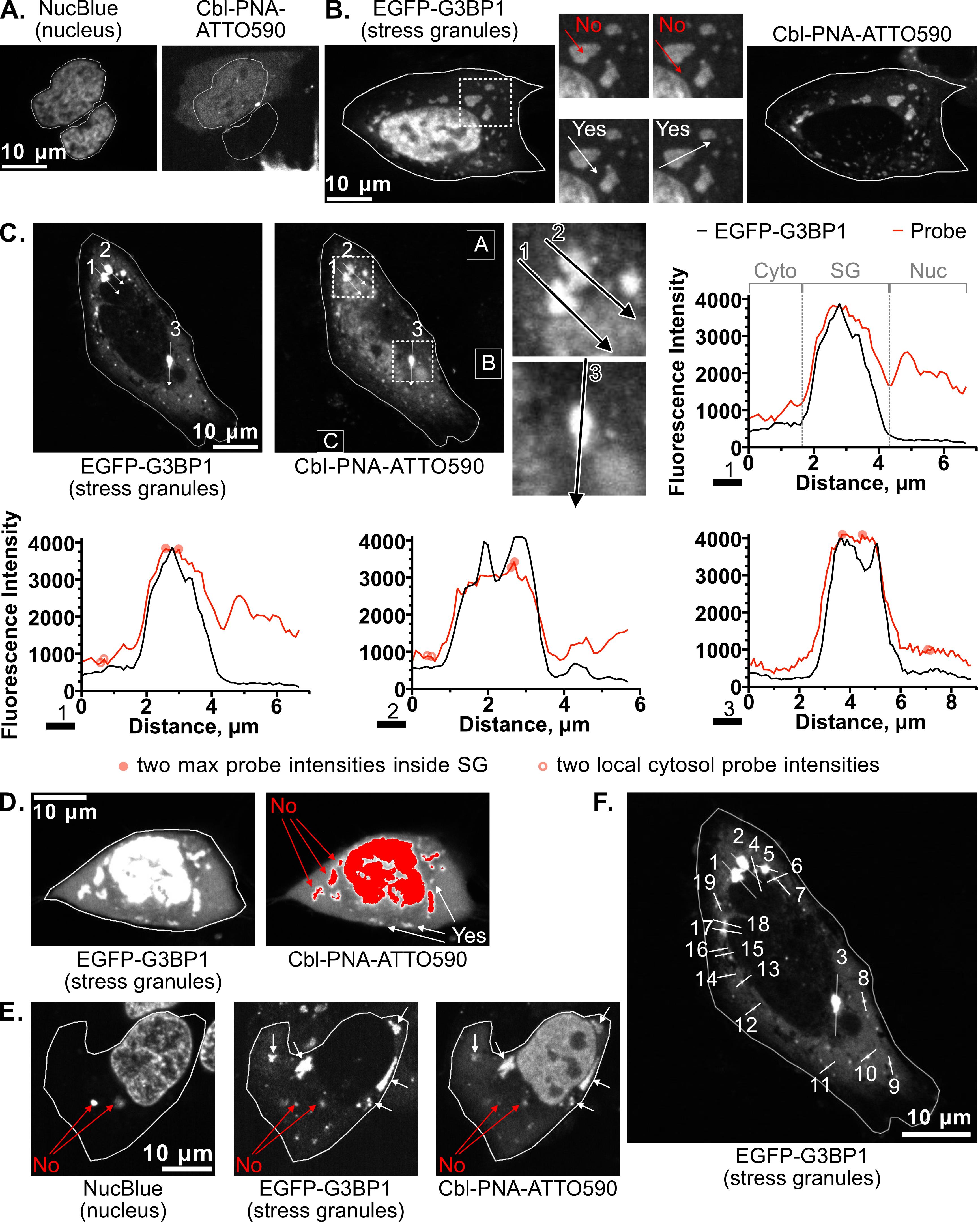
Figure 13. Explanation of data analysis for the SG assay. (A) Example images of two cells stained with NucBlue (left image) and beadloaded with 5 μM Cbl-PNA-ATTO590 (right image). Cells that are beadloaded show a bright nucleus in the probe channel (upper cell), while cells that are not beadloaded (lower cell) do not. Nuclei outlined in white are based on NucBlue signal. (B) Example images of a cell expressing EGFP-G3BP1 (left and middle images) and HaloTag-(1/2)NORAD-6xenv8-FL-3’antiPNA beadloaded with 5 μM Cbl-PNA-ATTO590 (right image). The dashed white rectangle indicates a zoomed-in portion (middle images). Line selections should begin in the cytosol, go through the center of the SG, and end in the cytosol for the best results. Cell outline in white. (C) Example images of a cell expressing EGFP-G3BP1 (left image) and ACTB-4xenv8-FL-3’antiPNA and beadloaded with 5 μM Cbl-PNA-ATTO590 (middle image). Cell outline in white. White arrows 1, 2, and 3 depict example line selections through SGs. White rectangles A, B, and C depict example rectangle selections outside of cells. The dashed white rectangle indicates a zoomed-in portion (right images). Plot on the far right of line selection 1 shows EGFP-G3BP1 signal in black and probe signal in red. The grey dashed lines show suggested segmentation of the line profile into the cytosol, SG, and nucleus, because this line selection begins in the cytosol, goes through the center of the SG, and ends in the nucleus. “Average” probe intensities in the local cytosol should only be chosen from segments of the line selection that correspond to the cytosol. Plots on the bottom of line selections 1, 2, and 3 show EGFP-G3BP1 signal in black and probe signal in red. Filled-in red circles show two maximum probe intensities inside the SG. Open red circles show two suggested “average” probe intensities in the local cytosol. (D) Example images of a cell expressing EGFP-G3BP1 (left image) and HaloTag-(1/2)NORAD-6xenv8-FL-3’antiPNA and beadloaded with 5 μM Cbl-PNA-ATTO590 (right image). Cell outline in white. Red color indicates pixels where the detector is saturated in the probe channel. SGs that contain saturated pixels in the probe channel should not be analyzed. Inclusion of these SGs could lead to falsely low enrichment values. (E) Example images of a cell stained with NucBlue (left image), expressing EGFP-G3BP1 and HaloTag-(1/2)NORAD-6xenv8-FL-3’antiPNA (middle image), and beadloaded with 5 μM Cbl-PNA-ATTO590 (right image). Cell outline in white. Red arrows denote spots that appear in all three channels. These spots should not be included in your analysis, as NucBlue should not stain SGs. When these spots are present, they typically appear in the perinuclear region. White arrows denote some of the SGs in this cell that would be analyzed. Note that their intensity in the probe channel varies significantly from SG to SG. (F) Repeat of the example image in C with white arrows depicting all the SGs that would be analyzed in this image. Cell outline in white. In all images, scale bar = 10 μm.
3. Split the channels of the image with Image ⟶ Color ⟶ Split Channels. Close channels other than the Riboglow probe channel and the SG marker channel, as you do not need them in analysis.
4. Use the line selection tool to draw a line across an SG in the SG marker channel: starting in the cytosol around the SG, going roughly through the center of the SG, and ending in the cytosol around the SG on the other side. Save the line selection in Analyze ⟶ Tools ⟶ ROI Manager. See Figure 13B.
Notes:
1. The center of the SG typically contains the maximum Riboglow probe intensities for downstream analysis.
2. The line selection can be drawn through the center of an SG differently, and each line will likely give slightly different enrichment values. Another group has, instead, successfully analyzed this assay using a selection area inside the SG (more likely to capture the absolute maximum intensity) compared to a selection area in the cytosol [20].
5. Use Analyze ⟶ Plot Profile to plot a line graph of the intensities in the SG marker channel as a function of position on the line selection.
6. Click on the Riboglow probe channel image. Click on the index for the line selection that you just created to populate this selection in this image. Use Analyze ⟶ Plot Profile to plot a line graph of the intensities of the Riboglow probe channel as a function of position on the line selection.
7. Combine the line profiles in the Plot Profile window by Data ⟶ Add from Plot… and select the other Plot Profile window from the drop-down menu. See line profiles for arrows 1, 2, and 3 in Figure 13C.
8. In this combined line profile, find the SG (as defined by high SG marker channel intensities) in the line profile. Now use your mouse to hover over points inside the SG on the line corresponding to the Riboglow probe channel. Find the two maximum intensities inside the SG. Record these two max intensities alongside other information like the image date, the Riboglow-tagged construct, the Riboglow probe, the Riboglow probe concentration, the cell number, and the SG number in a spreadsheet. See filled-in circles in Figure 13C and corresponding values in Figure 14A.
Notes:
1. If the maximum intensity saturates the detector in the probe channel, we recommend excluding this SG from analysis, as it may give falsely low enrichment ratios. See Figure 13D.
2. Selecting the two maximum intensities avoids issues caused by single-pixel intensity spikes that may give falsely high enrichment ratios.
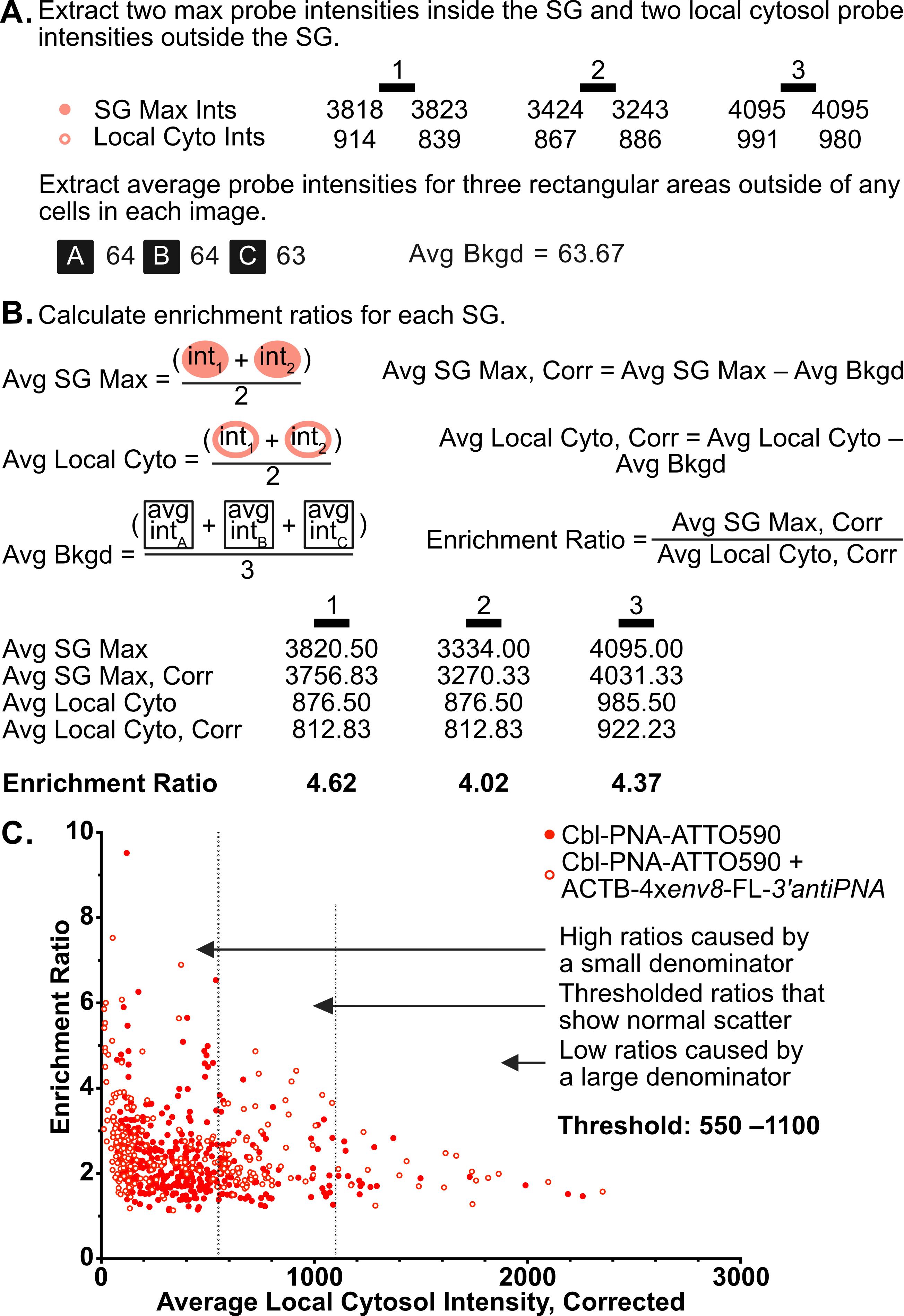
Figure 14. Explanation of calculations and thresholding for the SG assay. (A) Chosen probe intensities for the example line selections 1, 2, and 3, and the mean probe intensity for the example rectangular selections A, B, and C in Figure 13C. (B) Equations to calculate the average maximum probe intensity inside of the SG, the average local cytosol probe intensity outside of the SG, the average background probe intensity outside of any cells in the image, the background-corrected values of the average maximum probe intensity inside of the SG and the average local cytosol probe intensity outside of the SG, and the enrichment ratio. Using these equations and the values in A results in the calculated values shown here. (C) Scatter plot of enrichment ratios as a function of background-corrected average local cytosol probe intensity outside of the SG. Each point is an SG. Dashed lines and arrows depict the regions that correspond to artificially high enrichment ratios caused by a small background-corrected average local cytosol probe intensity, thresholded enrichment ratios that show normally distributed scatter, and artificially low enrichment ratios caused by a large background-corrected average local cytosol probe intensity. For this plot, the threshold would be set from 550 to 1,100 to only keep enrichment ratios that show a normally distributed scatter.
9. In this combined line profile, find two “average” intensities outside of the SG on the line corresponding to the Riboglow probe channel. Compare with the image and avoid any intensities that come from the nucleus (generally, high Riboglow probe intensity) or from the slightly dimmer perinuclear region where the Golgi typically forms (generally, low Riboglow probe intensity) and a higher likelihood of non-SG spots that appear in all three channels. “Average” cytosol intensities can both come from one side, or they can come from each side, of the SG. Avoid obvious peaks or valleys. Record these two “average” local cytosolic intensities in the spreadsheet. See open circles in Figure 13C and corresponding values in Figure 14A. See Figure 13E for an example of why we recommend avoiding the perinuclear region and spots that appear in all three channels.
Notes:
1. We selected and recorded only two “average” intensities from the local cytosol for each SG for speed of analysis. It is also possible to record all intensities from the local cytosol for each SG as we did in the original Riboglow paper’s SG enrichment ratio analysis [10,17].
2. Selection of two “average” values can be biased. We recommend blinding the analysis by asking a colleague to remove identifying information from image names and relabeling the images before analysis, if possible.
10. Repeat this process for all SGs in the cytosol that have well-defined edges and are at least 2 pixels × 2 pixels. See Figure 13F.
Note: RNA does not distribute to each SG uniformly in a cell, so the enrichment ratios of SGs within a cell will be different. See Figure 13E.
11. Use the rectangle selection tool to draw three boxes larger than 15 pixels × 15 pixels outside of any cells in the image. Use Analyze ⟶ Measure to determine the average Riboglow probe intensity in each box to correct for media autofluorescence and background detector noise. Record these mean background intensities in the spreadsheet. See rectangular selections A, B, and C in Figure 13C and corresponding values in Figure 14A.
Note: Media autofluorescence and background detector noise should not change much between images or days.
12. In the spreadsheet, calculate the average maximum probe intensity inside of each SG, the average local cytosol probe intensity outside of each SG, and the average probe intensity outside of any cells in the image. See the corresponding equations and calculation of these values in Figure 14B (from the data extracted from example images in Figure 13C).
13. In the spreadsheet, background-correct for media autofluorescence and detector noise by subtracting the average probe intensity outside of any cells in the image from both the average maximum probe intensity inside of each SG and the average local cytosol probe intensity outside of each SG. See the corresponding equations and calculation of these values in Figure 14B (from the data extracted from example images in Figure 13C).
14. In the spreadsheet, calculate the enrichment ratio by dividing the average maximum probe intensity inside of each SG by the average local cytosol probe intensity outside of each SG. See the corresponding equation and calculation of this value in Figure 14B (from the data extracted from example images in Figure 13C).
15. For each imaging set, plot the enrichment ratio as a function of the background-corrected average local cytosol probe intensity for each SG. Select a threshold that excludes enrichment ratios that are falsely high due to small denominators and excludes enrichment ratios that are falsely low due to large denominators. See Figure 14C for a visual explanation of how to choose a threshold.
Critical: This threshold should be applied to all data that you wish to compare with each other.
Note: We recommend using data from at least two or three different dishes for each condition to control for beadloading efficiency. We recommend analyzing approximately the same number of cells for each condition to control for cell-to-cell variation. We recommend analyzing approximately the same number of SGs for each condition so that no condition has drastically more statistical power than another condition.
16. If you would like, you can perform a Q-test on each thresholded condition to determine if the highest or lowest enrichment value is an outlier and should be removed.
Critical: Do not use a Q-test to remove more than one data point from each data set. You would need a different test to determine if more than one point is an outlier and should be removed.
17. Plot the data in a graphing software. Apply statistical tests with the following recommendations:
Critical:
1. Enrichment ratio data sets typically do not follow a normal distribution, in our hands. Therefore, all statistical tests must account for nonparametric distributions.
2. When comparing two data sets, apply a Kolmogorov-Smirnov test (nonparametric cumulative distribution t-test) to test if the distribution of enrichment ratios for Condition A is statistically higher or lower than the distribution of enrichment ratios for Condition B.
3. When comparing more than two data sets, apply a Kruskal-Wallis test (nonparametric one-way ANOVA) to test if the enrichment ratios for Condition A are statistically higher or lower than the enrichment ratios for Condition B or C.
Note: In the accompanying paper, we compared each condition against each other in our Kruskal-Wallis tests because we wanted to test if the conditions were different from each other. If you are only interested in testing if the conditions are different from another condition (often a negative control), you can perform the Kruskal-Wallis test comparing each condition against another selected condition.
U-body assay
1. Open the Nikon .nd2 images in Fiji/ImageJ2 using the Bio-Formats Importer.
2. Adjust the contrast, if necessary, with Image ⟶ Adjust ⟶ Brightness/Contrast. Confirm that the cell to be analyzed is expressing the U-body marker fusion protein, has U-bodies in the cytosol, and is beadloaded with the Riboglow probe. Throw out any cells that do not meet these three criteria.
3. Split the channels of the image with Image ⟶ Color ⟶ Split Channels. Close channels other than the Riboglow probe channel and the U-body marker channel, as you do not need them in analysis.
4. Open the Cell Counter window with Plugins ⟶ Cell Counter. Click on the U-body marker channel and click Initialize in the Cell Counter window. A new window will appear. Close the original U-body marker channel if it is still open.
5. Synchronize the initialized U-body marker channel and the Riboglow probe channel with Analyze ⟶ Tools ⟶ Synchronize Windows. Click Synchronize All in the pop-up window. A crosshair icon should now appear on both windows and follow your mouse movements.
6. Select Counter Type 1 in the Cell Counter window. Hover your mouse over U-bodies in the U-body marker channel, clicking when the U-body marker fusion protein and the Riboglow probe colocalize. A dot with a counter should appear at this location, and the number next to Counter Type 1 should increase. Repeat for all U-bodies where the U-body marker fusion protein and the Riboglow probe colocalize. See filled-in red triangles in Figure 15A.
Notes:
1. We recommend selecting minimum and maximum values that can be applied to the Riboglow probe channel in each image so that the analysis is internally consistent for what is determined “colocalized” vs. “not colocalized”. This can be done with Set in the Brightness & Contrast window.
2. This visual analysis of “colocalization” is slightly biased. We recommend blinding the analysis by asking a colleague to remove identifying information from image names and relabeling the images before analysis, if possible.
3. Object-based colocalization, like this, does not rely heavily on the intensity of pixels, beyond whether an object can be detected or not. Other colocalization values, like Mander’s overlap coefficient and Pearson correlation coefficient, depend on the intensity of pixels in the channels that you are comparing. Colocalization values that depend on intensity can easily be altered by the size of a U-body, the expression of the Riboglow-tagged construct, and the amount of Riboglow probe that entered the cell, all of which would increase the intensity. We recommend using object-based colocalization for this assay for this reason.
4. You could also apply the data analysis associated with the SG assay to determine the enrichment ratio of the Riboglow probe in U-bodies; however, the manual analysis to determine the enrichment ratio is much more time-intensive than this object-based cytosolic colocalization analysis. We did not use the object-based cytosolic colocalization analysis with the SG assay because the Riboglow probe accumulates in SGs in the absence of expression of the RNA tag at a much higher rate than it does with U-bodies, interestingly.
7. Select Counter Type 2 in the Cell Counter window. Hover your mouse over U-bodies in the U-body marker channel, clicking when the U-body marker fusion protein does not colocalize with the Riboglow probe. A different colored dot with a counter should appear at this location, and the number next to Counter Type 2 should increase. Repeat this for all U-bodies where the U-body marker fusion protein does not colocalize with the Riboglow probe. See open red triangles in Figure 15A.
8. Record the number of U-bodies showing colocalization with the Riboglow probe (Counter Type 1) and the number of U-bodies not showing colocalization (Counter Type 2) alongside other information like the image date, the Riboglow-tagged construct, the Riboglow probe, the Riboglow probe concentration, and the cell number in a spreadsheet.
9. Close all images and counter windows to avoid confusion and repeat this process for all other images to be analyzed.
10. In the spreadsheet, calculate the percent cytosolic colocalization by dividing the number of U-bodies showing colocalization with the Riboglow probe by the total number of U-bodies in the cell (the sum of the number of U-bodies showing colocalization with the Riboglow probe and the number of U-bodies not showing colocalization). See Figure 15B.
Note: We did not find any need to apply a threshold to average cytosolic probe intensity (averaged from average probe intensities in three rectangular selections in the cytosol outside of U-bodies). See Figure 15C. However, if you have a condition where the total number of U-bodies decreases to a low number (~5 or less), it may be worth plotting the percent cytosolic colocalization as a function of the total number of U-bodies. Low denominators may interfere with the natural spread of the data. In this case, a threshold should be applied to exclude these values, similar to the threshold applied in the SG assay. Ensure that this threshold is applied to all data sets that you wish to compare.
11. If you would like, you can perform a Q-test on each thresholded condition to determine if the highest or lowest enrichment value is an outlier and should be removed.
Critical: Do not use a Q-test to remove more than one data point from each data set. You would need a different test to determine if more than one point is an outlier and should be removed.
12. Plot the data in a graphing software. Apply statistical tests with the following recommendations:
Critical:
1. Some sets of cytosolic colocalization percentages do not follow a normal distribution, in our hands. Therefore, all statistical tests must account for nonparametric distributions. When comparing two data sets, apply a Kolmogorov-Smirnov test (nonparametric cumulative distribution t-test) to test if the distribution of enrichment ratios for Condition A is statistically higher or lower than the distribution of enrichment ratios for Condition B.
2. When comparing more than two data sets, apply a Kruskal-Wallis test (nonparametric one-way ANOVA) to test if the enrichment ratios for Condition A are statistically higher or lower than the enrichment ratios for Condition B or C.
Note: In the original publication where this protocol was applied [12], we compared each condition against each other using Kruskal-Wallis tests because we wanted to test if the conditions were different from each other. If you are only interested in testing if the conditions are different from one another (often a negative control), you can perform the Kruskal-Wallis test comparing each condition against one other selected condition.
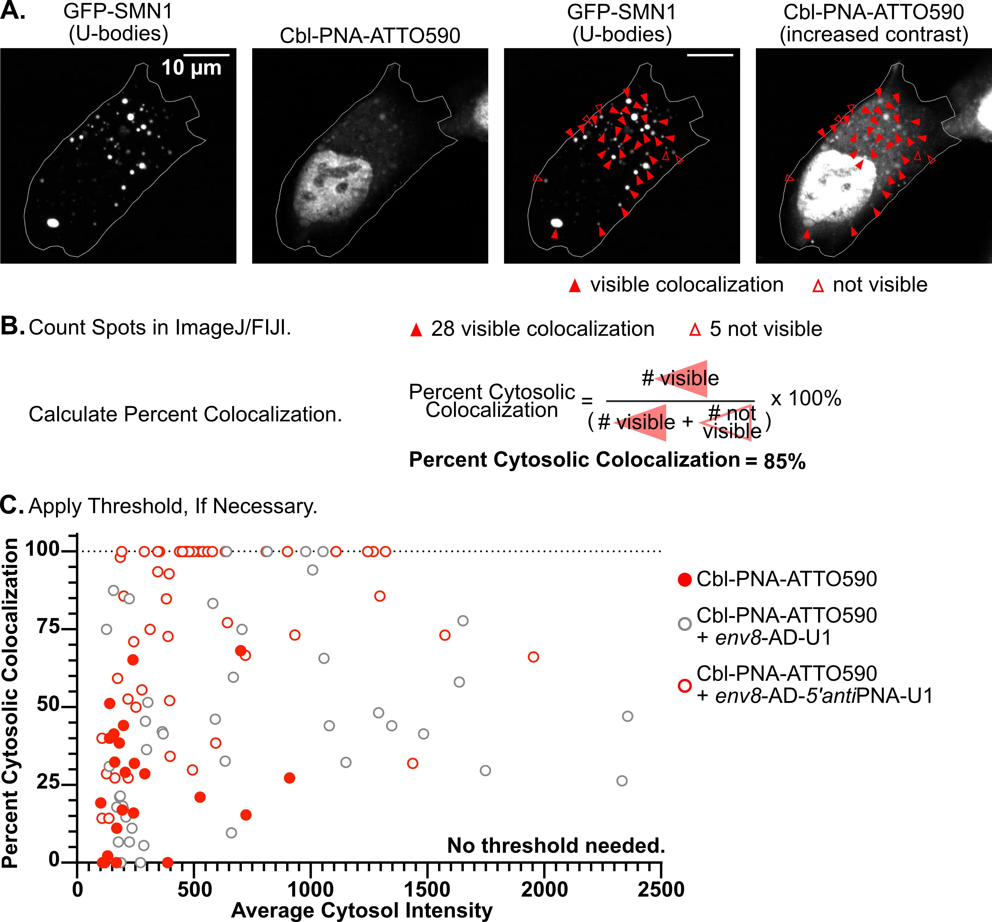
Figure 15. Explanation of data analysis and calculation for the U-body assay. (A) Example images of a cell expressing EGFP-SMN1 (first and third images from the left) and env8-AD-5’antiPNA-U1 and beadloaded with 50 μM Cbl-PNA-ATTO590 (second and fourth images from the left). Cell outline in white. Filled-in red triangles indicate U-bodies that visually contain signal in the probe channel. Open red triangles indicate U-bodies that do not visually contain a signal in the probe channel. Scale bar = 10 μm. (B) Values from the example images above and the calculated percent cytosolic colocalization. (C) Scatter plot of percent cytosolic colocalization as a function of average cytosol probe intensity. Each point is a cell. Horizontal dashed line indicates 100% colocalization. The plot shows normal scattering, so no threshold was applied to the average cytosol probe intensity.
General notes and troubleshooting
Troubleshooting
This list of troubleshooting suggestions is not an exhaustive list, but it intends to list problems or possible causes that would not be easily solved by searching the Internet.
Making homemade imaging dishes
Problem: Glass does not adhere well to the dish.
Possible cause: Tissue culture–treated cell culture dishes with thicker polystyrene on the bottom of the dish result in polystyrene burrs that do not allow the glass to make good contact with the plastic of the dish.
Solution: Burrs must be sanded off before continuing. If sanding with sandpaper is required, rinse the punched and sanded dishes in distilled water a few times to remove any particles from the sandpaper. Allow to air dry before continuing.
Possible cause: There is an insufficient amount of silicone elastomer to adhere the coverslip to the dish.
Solution: Make a full seal between the edges of the glass coverslip and the bottom of the cell culture dishes around the punched hole with the silicone elastomer. We find that using a 1,000 μL pipette tip to dot the silicone elastomer in a ring around the punched hole before carefully placing a glass coverslip on the top of the upside-down cell culture dish works best.
Problem: Few cells are present on the glass coverslip on the day of imaging before beadloading.
Possible cause: Cells do not adhere well to the glass.
Solution: Coat the glass with poly-D-lysine, fibronectin, collagen, or other coating agent (according to the cell line that you are using) for better adhesion.
Plating and transfecting cells
Problem: Cells are not predictably growing or transfecting.
Possible cause: Cells are contaminated with mycoplasma.
Solution: Test cells for mycoplasma with a mycoplasma testing kit according to the manufacturer’s instructions. If contaminated, fully replace all media and reagents, treat cells or begin again from a mycoplasma-free vial of cells, and practice sterile technique before continuing.
Possible cause: Cells are too sparsely or too densely plated during times between imaging experiments.
Solution: We find that U-2 OS cells behave more predictably (growth rate, transfection efficiency) if they have been passaged at least once since cryo-storage and have been consistently plated at ≥15% confluency and passaged before ≤90% confluency.
Problem: Cells are unevenly spaced in the imaging dish.
Possible cause: Cells were not sufficiently mixed before plating.
Solution: Prepare an N× batch of cells for N dishes in a 15 or 50 mL conical tube, adding fresh media up to the final media volume, resuspending the cells by pipetting, and plating 2 mL into each imaging dish.
Possible cause: Dishes were placed on an uneven surface while cells were adhering.
Solution: Find a level surface and allow the cells to settle for 20 min before moving them to the incubator.
Problem: Cells are poorly transfected.
Possible cause: Cells were too sparsely or too densely plated.
Solution: In the context of this assay, we see the best transfection efficiencies when cells are ~40% confluent on the day of transfection. If cells are significantly lower confluency (15%), wait until they reach at least 30% confluency before transfecting. If cells are amenable, transfection may also be done on the day of plating (day 1) to significantly increase the transfection efficiency due to the increased number of cells present at the time of transfection. In this case, imaging should still be performed 24 h later, and more cells should be plated on Day 1 to account for the decreased time between plating and imaging.
Possible cause: Lipofection particles were inefficiently made.
Solution: We see slightly better transfection efficiencies when using smaller tubes (0.6 mL), lower OptiMEM volumes (25 or 50 μL), and midiprepped DNA. We also see better transfection efficiencies when the lipofection mixture is allowed to incubate for longer times (30 min).
Beadloading
Problem: Beads do not efficiently cover cells in the dish.
Possible cause: Beads are damp.
Solution: During assembly of the beadloader, ensure that washed beads are fully dry by gently shaking the beadloader and confirming that there are no chunks of beads before continuing.
Solution: Keep the beadloader in desiccant whenever it is not in use. Replace the desiccant as often as necessary.
Problem: Few cells remain after beadloading.
Possible cause: Cells are too dense at the time of beadloading.
Solution: Adjust cell plating numbers to achieve 50%–70% confluency on the day of imaging. Beadloading dishes with ≥90% confluency often results in cells peeling off the dish in large sections.
Possible cause: Beadloading was performed with too much force.
Solution: Use less force when beadloading cells, tap the cells fewer times, or a combination of the two.
Possible cause: Too many rinses before imaging.
Solution: Although most issues with beadloading occur before the rinsing step, excess rinsing will reduce the number of beadloaded cells that stay adhered to the dish. If necessary, rinse fewer times and avoid areas with beads when imaging to mitigate an increased background signal caused by leftover beads.
Problem: Cells do not appear properly beadloaded by fluorescence microscopy.
Possible cause: Too little or too much probe solution to cover the cells in the imaging area.
Solution: Increase the volume of probe solution to cover most/all the cells in the imaging area. For purchased imaging dishes that have a larger glass surface area, use ~20 μL of probe solution. If too much probe solution is used, the beads will make poor contact with the cells. In either case, keep the probe at the same concentrations as those recommended in the protocol. Keep this volume consistent between dishes, as it can impact the concentration of the probe that is beadloaded into cells.
Possible cause: Beadloading was performed with too little or too much force.
Solution: Tapping harder will increase the amount of probe in cells and the percent of cells that get beadloaded. Tapping too softly will yield poorly beadloaded cells with a low probe signal. Tapping too hard will make beadloaded cells detach from the dish, leaving only poorly beadloaded cells with low probe signal. Practice the force required for beadloading on an ordinary lab scale. We typically use ~30–70 g of force.
Problem: Beadloading is inconsistent between dishes.
Possible cause: Beadloading in a well plate instead of a single dish.
Solution: We find that beadloading in a well plate feels clunky, which makes it difficult to beadload only one well of the plate at a time. Beadloading a single 35 mm dish works best for us.
Possible cause: Beadloading force is inconsistent between dishes.
Solution: We recommend regularly practicing the force necessary to beadload cells, especially when new to the technique or when there has been a long time between uses of the technique. We regularly practiced the force necessary just before beadloading samples.
Imaging
Problem: Images look blurry.
Possible cause: The glass coverslip may not match the recommended glass thickness for use with the objective.
Solution: Switch to a #1.5 (0.17 mm) glass coverslip to best match the recommended glass thickness for most oil objectives.
Possible cause: You are trying to image through the silicone elastomer used to make the homemade imaging dishes.
Solution: Avoid areas of the glass coverslip with silicone elastomer. When making homemade imaging dishes, reduce the amount of silicone elastomer that is used to adhere the glass coverslip to the dish to increase the total usable area of the imaging dish.
Problem: Images have a high background signal.
Possible cause: The imaging media has FBS in it.
Solution: We recommend using FluoroBrite DMEM + 10% FBS as the imaging media because it best mimics the cell culture media, and we find that it keeps cells happiest during longer imaging sessions (~2 h). However, if the background signal is too high, consider removing the FBS or using computational methods to correct for the high background.
Possible cause: There are many glass beads nearby.
Solution: Glass beads show high fluorescence. Move to areas of the dish that have fewer glass beads. Next time, add another rinsing step after beadloading, ensuring that the dish is angled to move all leftover beads to one portion of the dish.
Problem: Cells are not forming SGs or U-bodies.
Possible cause: The stressor may have degraded.
Solution: When making concentrated solutions of stressor, make single-use aliquots. We have noticed some issues with delayed formation or lack of formation of SGs or U-bodies with aliquots that are over a year old or have undergone multiple freeze-thaw cycles.
Possible cause: Your cells are not at the correct temperature and CO2.
Solution: SG formation rate is dependent on both temperature and CO2. Ensure that you keep cells at 37 °C and 5% CO2 before and during imaging, if possible.
Possible cause: Your cells are much more or much less confluent than normal.
Solution: We have noticed that cell confluency impacts the ability of cells to form SGs and U-bodies. If possible, give your cells some more time to form SGs and U-bodies.
Problem: Cells die before imaging or early on in imaging.
Possible cause: The imaging media cannot buffer CO2, so the media is acidifying.
Solution: In this protocol, we recommend FluoroBrite DMEM + 10% FBS as the imaging media to mimic the cell culture media. FluoroBrite DMEM can buffer CO2, while other common imaging medium like L15 cannot.
Possible cause: The stressor may be too strong for the cells.
Solution: In this protocol, we use U-2 OS cells, and our concentrations and incubation time for the stressors have been validated in this cell line. If you use a different cell line or express an RNA of interest that may impact the cells’ ability to handle stress, you may need to modulate the concentration of the stressor or its incubation time on the cells.
Validation of protocol
This protocol (or parts of it) has been used and validated in the following research articles:
1. Cobalamin-PNA probe synthesis
• Wierzba et al. [27]. Vitamin B12 – Peptide Nucleic Acid Conjugates. Methods in Molecular Biology.
• Wierzba et al. [12]. Unveiling the Promise of Peptide Nucleic Acids as Functional Linkers for an RNA Imaging Platform. RSC Chemical Biology (Figure 1; Supporting Information: Probe synthesis and characterization).
2. Fluorescence turn-on assay
• Wierzba et al. [12]. Unveiling the Promise of Peptide Nucleic Acids as Functional Linkers for an RNA Imaging Platform. RSC Chemical Biology (Figure 3; Figure 4D–E; Figure 5; Supporting Information: Methods 3.2).
3. SHAPE assay
• Das et al. [25]. SAFA: semi-automated footprinting analysis software for high-throughput quantification of nucleic acid footprinting experiments. RNA.
• Stoddard et al. [24]. Ligand-dependent folding of the three-way junction in the purine riboswitch. RNA (Figures 2–4).
• Wierzba et al. [12]. Unveiling the Promise of Peptide Nucleic Acids as Functional Linkers for an RNA Imaging Platform. RSC Chemical Biology (Figure 2; Figure 4B–C; Supporting Figures S5–S7).
• Wilkinson et al. [23]. Selective 2’-hydroxyl acylation analyzed by primer extension (SHAPE): quantitative RNA structure analysis at single nucleotide resolution. Nature Protocols.
4. SG assay
• Braselmann et al. [10]. A multicolor riboswitch-based platform for imaging of RNA in live mammalian cells. Nature Chemical Biology (Figures 3–4; Supplementary Table 12; Supplementary Figures 13–22; Supplementary Figure 26).
• Braselmann and Palmer. [17]. Chapter 15: A multicolor riboswitch-based platform for imaging of RNA in live mammalian cells. Methods in Enzymology.
• Wierzba et al. [12]. Unveiling the Promise of Peptide Nucleic Acids as Functional Linkers for an RNA Imaging Platform. RSC Chemical Biology (Figure 6; Supporting Figures S10–S11; Supporting Table S5; Supporting Methods 3.3–3.4).
• Many other groups have used a version of the SG assay to test their fluorescent RNA tags. The full list of papers to date is given in the Background section.
5. U-body assay
• Braselmann et al. [10]. A multicolor riboswitch-based platform for imaging of RNA in live mammalian cells. Nature Chemical Biology (Figure 5; Supplementary Table 12; Supplementary Figures 13, 28–31).
• Braselmann and Palmer [17]. Chapter 15: A multicolor riboswitch-based platform for imaging of RNA in live mammalian cells. Methods in Enzymology.
• Wierzba et al. [12]. Unveiling the Promise of Peptide Nucleic Acids as Functional Linkers for an RNA Imaging Platform. RSC Chemical Biology (Figure 7; Supporting Figure S12; Supporting Table S5; Supporting Methods 3.5–3.6).
Acknowledgments
A.J.W., Cbl-PNA probe synthesis and fluorescence turn-on assay; E.M.R., SG and U-body assays; S.R.L., SHAPE assay. A.J.W., E.M.R., S.R.L.: writing – original draft. A.J.W., E.M.R., R.T.B., A.E.P.: writing – review and editing. R.T.B., A.E.P.: supervision, funding acquisition. Financial support: R01 GM133184 (A.E.P. and R.T.B.), R35 GM139644 (A.E.P.), R35 GM152029 (R.T.B.), T32 GM065103 (E.M.R., S.R.L.), F31 5F31ES033919 (E.M.R.), Polish National Agency for Academic Exchange PPN/BEK/2020/1/00219/U/0000 (A.J.W.). We thank the Shared Instruments Pool (RRID: SCR_018986) of the Department of Biochemistry at the University of Colorado Boulder for the use of the Typhoon 5. The Typhoon 5 is funded by NIH Shared Instrumentation Grant S10OD034218-01. The imaging work was performed at the BioFrontiers Institute’s Advanced Light Microscopy Core (RRID: SCR_018302). Laser scanning confocal microscopy was performed on a Nikon A1R microscope supported by NIST-CU Cooperative Agreement award number 70NANB15H226. We would like to thank Dr Joe Dragavon of the BioFrontiers Institute Advanced Light Microscopy Core for assistance with microscopy. We would like to acknowledge the University of Colorado Biochemistry Cell Culture Core Facility, especially Dr Theresa Nahreini, for providing resources and support for all our cell work. All protocol elements were validated in Wierzba et al. [12] RSC Chem Biol., 2025, 6, 249–262. Previous work from which the protocol was developed and/or modified include Braselmann et al. [10] Nature Chem Biol., 2018, 14, 964–971 and Braselmann et al. [17] Methods Enzymol., 2020, 641, 343–372.
Competing interests
The authors declare the following competing financial interest(s): R.T.B. serves on the Scientific Advisory Boards of SomaLogic and MeiraGTx.
References
- Tutucci, E., Vera, M., Biswas, J., Garcia, J., Parker, R. and Singer, R. H. (2018). An improved MS2 system for accurate reporting of the mRNA life cycle. Nat Methods. 15(1): 81–89. https://doi.org/10.1038/nmeth.4502
- Tutucci, E., Livingston, N. M., Singer, R. H. and Wu, B. (2018). Imaging mRNA In Vivo, from Birth to Death. Annu Rev Biophys. 47(1): 85–106. https://doi.org/10.1146/annurev-biophys-070317-033037
- Wu, B., Miskolci, V., Sato, H., Tutucci, E., Kenworthy, C. A., Donnelly, S. K., Yoon, Y. J., Cox, D., Singer, R. H. and Hodgson, L. (2015). Synonymous modification results in high-fidelity gene expression of repetitive protein and nucleotide sequences. Genes Dev. 29(8): 876–886. https://doi.org/10.1101/gad.259358.115
- Garcia, J. F. and Parker, R. (2015). MS2 coat proteins bound to yeast mRNAs block 5’ to 3’ degradation and trap mRNA decay products: implications for the localization of mRNAs by MS2-MCP system. RNA. 21(8): 1393–1395. https://doi.org/10.1261/rna.051797.115
- Garcia, J. F. and Parker, R. (2016). Ubiquitous accumulation of 3′ mRNA decay fragments in Saccharomyces cerevisiae mRNAs with chromosomally integrated MS2 arrays. RNA. 22(5): 657–659. https://doi.org/10.1261/rna.056325.116
- Chen, X., Zhang, D., Su, N., Bao, B., Xie, X., Zuo, F., Yang, L., Wang, H., Jiang, L., Lin, Q., et al. (2019). Visualizing RNA dynamics in live cells with bright and stable fluorescent RNAs. Nat Biotechnol. 37(11): 1287–1293. https://doi.org/10.1038/s41587-019-0249-1
- Sunbul, M., Lackner, J., Martin, A., Englert, D., Hacene, B., Grün, F., Nienhaus, K., Nienhaus, G. U. and Jäschke, A. (2021). Super-resolution RNA imaging using a rhodamine-binding aptamer with fast exchange kinetics. Nat Biotechnol. 39(6): 686–690. https://doi.org/10.1038/s41587-020-00794-3
- Paige, J. S., Wu, K. Y. and Jaffrey, S. R. (2011). RNA Mimics of Green Fluorescent Protein. Science. 333(6042): 642–646. https://doi.org/10.1126/science.1207339
- Dolgosheina, E. V., Jeng, S. C. Y., Panchapakesan, S. S. S., Cojocaru, R., Chen, P. S. K., Wilson, P. D., Hawkins, N., Wiggins, P. A. and Unrau, P. J. (2014). RNA Mango Aptamer-Fluorophore: A Bright, High-Affinity Complex for RNA Labeling and Tracking. ACS Chem Biol. 9(10): 2412–2420. https://doi.org/10.1021/cb500499x
- Braselmann, E., Wierzba, A. J., Polaski, J. T., Chromiński, M., Holmes, Z. E., Hung, S.-T., Batan, D., Wheeler, J. R., Parker, R., Jimenez, R., et al. (2018). A multicolor riboswitch-based platform for imaging of RNA in live mammalian cells. Nat Chem Biol. 14(10): 964–971. https://doi.org/10.1038/s41589-018-0103-7
- Polaski, J. T., Webster, S. M., Johnson, J. E. and Batey, R. T. (2017). Cobalamin riboswitches exhibit a broad range of ability to discriminate between methylcobalamin and adenosylcobalamin. J Biol Chem. 292(28): 11650–11658. https://doi.org/10.1074/jbc.M117.787176
- Wierzba, A. J., Richards, E. M., Lennon, S. R., Batey, R. T. and Palmer, A. E. (2025). Unveiling the promise of peptide nucleic acids as functional linkers for an RNA imaging platform. RSC Chem Biol. 6(2): 249–262. https://doi.org/10.1039/D4CB00274A
- Nielson, P. E., Egholm, M., Berg, R. H. and Buchardt, O. (1991). Sequence-Selective Recognition of DNA by Strand Displacement with a Thymine-Substituted Polyamide. Science. 254(5037): 1497–1500. https://doi.org/10.1126/science.1962210
- Mollet, S., Cougot, N., Wilczynska, A., Dautry, F., Kress, M., Bertrand, E. and Weil, D. (2008). Translationally Repressed mRNA Transiently Cycles through Stress Granules during Stress. Mol Biol Cell. 19(10): 4469–4479. https://doi.org/10.1091/mbc.e08-05-0499
- Nelles, D. A., Fang, M. Y., O’Connell, M. R., Xu, J. L., Markmiller, S. J., Doudna, J. A. and Yeo, G. W. (2016). Programmable RNA Tracking in Live Cells with CRISPR/Cas9. Cell. 165(2): 488–496. https://doi.org/10.1016/j.cell.2016.02.054
- Wu, J., Zaccara, S., Khuperkar, D., Kim, H., Tanenbaum, M. E. and Jaffrey, S. R. (2019). Live imaging of mRNA using RNA-stabilized fluorogenic proteins. Nat Methods. 16(9): 862–865. https://doi.org/10.1038/s41592-019-0531-7
- Braselmann, E. and Palmer, A. E. (2020). A multicolor riboswitch-based platform for imaging of RNA in live mammalian cells. Methods Enzymol. 641: 343–372. https://doi.org/10.1016/bs.mie.2020.03.004
- Li, X., Kim, H., Litke, J. L., Wu, J. and Jaffrey, S. R. (2020). Fluorophore-Promoted RNA Folding and Photostability Enables Imaging of Single Broccoli-Tagged mRNAs in Live Mammalian Cells. Angew Chem Int Ed. 59(11): 4511–4518. https://doi.org/10.1002/anie.201914576
- Wang, Q., Xiao, F., Su, H., Liu, H., Xu, J., Tang, H., Qin, S., Fang, Z., Lu, Z., Wu, J., et al. (2022). Inert Pepper aptamer-mediated endogenous mRNA recognition and imaging in living cells. Nucleic Acids Res. 50(14): e84. https://doi.org/10.1093/nar/gkac368
- Sarfraz, N., Moscoso, E., Oertel, T., Lee, H. J., Ranjit, S. and Braselmann, E. (2023). Visualizing orthogonal RNAs simultaneously in live mammalian cells by fluorescence lifetime imaging microscopy (FLIM). Nat Commun. 14(1): 867. https://doi.org/10.1038/s41467-023-36531-y
- Jarmoskaite, I., AlSadhan, I., Vaidyanathan, P. P. and Herschlag, D. (2020). How to measure and evaluate binding affinities. eLife. 9: e57264. https://doi.org/10.7554/eLife.57264
- Merino, E. J., Wilkinson, K. A., Coughlan, J. L. and Weeks, K. M. (2005). RNA Structure Analysis at Single Nucleotide Resolution by Selective 2′-Hydroxyl Acylation and Primer Extension (SHAPE). J Am Chem Soc. 127(12): 4223–4231. https://doi.org/10.1021/ja043822v
- Wilkinson, K. A., Merino, E. J. and Weeks, K. M. (2006). Selective 2′-hydroxyl acylation analyzed by primer extension (SHAPE): quantitative RNA structure analysis at single nucleotide resolution. Nat Protoc. 1(3): 1610–1616. https://doi.org/10.1038/nprot.2006.249
- Stoddard, C. D., Gilbert, S. D. and Batey, R. T. (2008). Ligand-dependent folding of the three-way junction in the purine riboswitch. RNA. 14(4): 675–684. https://doi.org/10.1261/rna.736908
- Das, R., Laederach, A., Pearlman, S., Herschlag, D. and Altman, R. B. (2005). SAFA: Semi-automated footprinting analysis software for high-throughput quantification of nucleic acid footprinting experiments. RNA. 11(3): 344–354. https://doi.org/10.1261/rna.7214405
- Park, J. G. and Palmer, A. E. (2015). Verifying the Function and Localization of Genetically Encoded Ca2+ Sensors and Converting FRET Ratios to Ca2+ Concentrations. Cold Spring Harb Protoc. 2015(1): pdb.prot076547. https://doi.org/10.1101/pdb.prot076547
- Wierzba, A. J., Wojciechowska, M., Trylska, J. and Gryko, D. (2021). Vitamin B12 – Peptide Nucleic Acid Conjugates. In W. M. Hussein, R. J. Stephenson, and I. Toth (Eds.), Peptide Conjugation (Vol. 2355, pp. 65–82). New York, NY: Springer US. https://doi.org/10.1007/978-1-0716-1617-8_7
Article Information
Publication history
Received: Jun 5, 2025
Accepted: Aug 19, 2025
Available online: Sep 9, 2025
Published: May 5, 2026
Copyright
© 2026 The Author(s); This is an open access article under the CC BY-NC license (https://creativecommons.org/licenses/by-nc/4.0/).
How to cite
Wierzba, A. J., Richards, E. M., Lennon, S. R., Batey, R. T. and Palmer, A. E. (2026). Enhancement of RNA Imaging Platforms by the Use of Peptide Nucleic Acid-Based Linkers. Bio-protocol 16(9): e5453. DOI: 10.21769/BioProtoc.5453.
Category
Biochemistry > RNA
Molecular Biology > RNA > RNA localisation
Do you have any questions about this protocol?
Post your question to gather feedback from the community. We will also invite the authors of this article to respond.