- Protocols

- Articles and Issues
- For Authors
- About
- Become a Reviewer

Protein Turnover Dynamics Analysis With Subcellular Spatial Resolution
(*contributed equally to this work) Published: Vol 15, Iss 15, Aug 5, 2025 DOI: 10.21769/BioProtoc.5409 Views: 2406
Reviewed by: David PaulAnonymous reviewer(s)
Original research article
The authors used this protocol in:

Mar 2024

Protocol Collections
Comprehensive collections of detailed, peer-reviewed protocols focusing on specific topics


Related protocols
Abstract
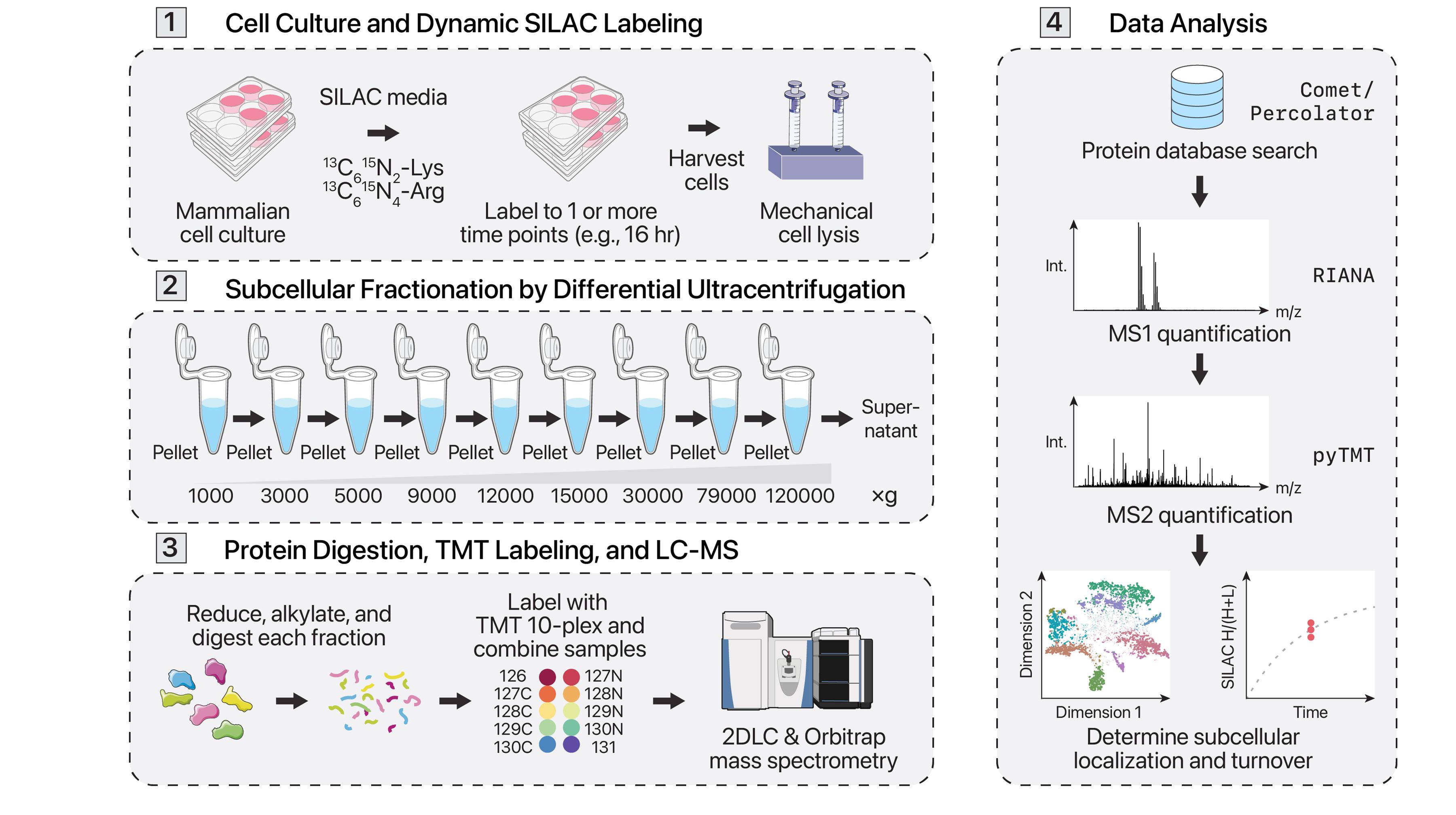
Protein synthesis and degradation (i.e., turnover) forms an important part of protein homeostasis and has been implicated in many age-associated diseases. Different cellular locations, such as organelles and membraneless compartments, often contain individual protein quality control and degradation machineries. Conventional methods to assess protein turnover across subcellular compartments require targeted genetic manipulation or isolation of specific organelles. Here we describe a protocol for simultaneous proteome localization and turnover (SPLAT) analysis, which combines protein turnover measurements with unbiased subcellular spatial proteomics to measure compartment-specific protein turnover rates on a proteome-wide scale. This protocol utilizes dynamic stable isotope labeling of amino acids in cell culture (dynamic SILAC) to resolve the temporal information of protein turnover and multi-step differential ultracentrifugation to assign proteins to multiple subcellular localizations. We further incorporate 2D liquid chromatography fractionation to greatly increase analytical depth while multiplexing with tandem mass tags (TMT) to reduce acquisition time 10-fold. This protocol resolves the spatial and temporal distributions of proteins and can also reveal temporally distinct spatial localizations within a protein pool.
Key features
• Captures protein turnover rates and subcellular localization of proteins.
• Hyperplexing of dynamic SILAC and TMT LOPIT-DC in MS1 and MS2 level data.
• Sample collection and processing can be completed within 1 week.
• Allows comparison of organellar proteome turnover rates.
Keywords: ProteomicsGraphical overview
Background
Mass spectrometry–based proteomics has traditionally focused on comparing steady-state protein abundances between various conditions to describe the biological processes occurring. However, protein abundances alone cannot provide a comprehensive description of the ongoing cellular processes. During a particular cellular process, protein abundance may stay consistent while protein utilization is altered. An alternative measure of protein utilization is protein turnover, or the replacement of existing protein with newly synthesized protein. The rate at which this occurs can be measured via dynamic stable isotope labeling of amino acids in cell culture (dynamic SILAC) [1–3]. Dynamic SILAC involves introducing heavy stable isotope–labeled essential amino acids, commonly lysine and/or arginine, into cells. The essential amino acids taken into cells are incorporated into newly synthesized proteins. The heavily labeled proteins and peptides can then be distinguished by their mass shifts and quantified via mass spectrometry. Protein turnover can then be calculated from the fractional incorporation of the heavy isotope into the total protein pool prior to full equilibration.
The turnover of proteins is influenced by their subcellular localization. For instance, proteins localized to the endomembrane system may be degraded via endoplasmic reticulum–associated protein degradation (ERAD) or autophagy, whereas mitochondrial matrix proteins may be degraded via a system of intra-mitochondrial AAA+ proteases that share homology with bacterial protease systems. Furthermore, it has become increasingly apparent that protein regulation can occur spatially rather than through changes in total abundance [4,5]. Mass spectrometry–based subcellular spatial proteomics methods have been developed that can assess the spatial distribution of proteins. These methods can largely be categorized as proximity labeling vs. ultracentrifugation-based methods. Ultracentrifugation-based protocols, including protein correlation profiling (PCP) [6], localization of organelle proteins by isotope tagging (LOPIT) and its variants [7–9], SubCellBarCode [6], and dynamic organellar maps (DOM) [10,11], have been widely used to identify protein subcellular localization and relocalization in cell models. These methods typically involve gently lysing cells while preserving organellar structures, then fractionating the cell lysate into multiple fractions with ultracentrifugation. Protein localization is then predicted by using a machine learning program from the distribution profile of a protein over the set of fractions compared to the distribution profiles for protein organelle markers.
Few methods exist that can orthogonally measure protein localization and turnover to provide a comprehensive protein spatial-temporal analysis. The conventional approach involves targeted isolation of specific organelles, such as the mitochondrion, to measure the half-life of organellar proteins [12]. Another method involves the targeted exogenous expression of a mitochondrially localized APEX protein to proximally label and pull down mitochondrial proteins, then measure their dynamic SILAC incorporation [13]. These methods, however, fall short of a global investigation of turnover across spatial locales. In a recent work, we presented an improved strategy that combines orthogonal approaches to simultaneously measure turnover and predict protein subcellular localization across many different organelles and compartments [14]. This method, termed simultaneous proteome localization and turnover (SPLAT), informs on the spatial distribution and temporal alterations in protein regulation by combining differential ultracentrifugation-based LOPIT (LOPIT-DC) and dynamic SILAC within one experiment. This is performed using a hyperplexing protocol that encodes SILAC and TMT information in MS1 and MS2 scans, as detailed below.
Materials and reagents
Biological materials
1. AC16 cell line (Milipore, catalog number: SCC109)
Reagents
1. PBS (Fisher, catalog number: BSSPBS1X6)
2. Trypsin-EDTA (Corning, catalog number: 25-053-CI)
3. HALT Protease and Phosphatase kit (Thermo, catalog number: PI78442)
4. HEPES (Thermo, catalog number: 11344041)
5. Sucrose (Thermo, catalog number: A15583.36)
6. Magnesium acetate (Fisher, catalog number: AC212552500)
7. DMEM-F12 for SILAC (Fisher, catalog number: PI88370)
8. Fetal bovine serum, dialyzed (Fisher, catalog number: A3382001)
9. 13C615N2 L-Lysine 2HCl (Fisher, catalog number: PI88209)
10. 13C615N4 L-Arginine HCl (Fisher, catalog number: PI89990)
11. DMEM-F12 (Fisher, catalog number: 10-090-CV)
12. Fetal bovine serum (Fisher, catalog number: A5209402)
13. LC-MS grade H2O (Sigma, catalog number: 7732-18-5)
14. SDS (Sigma Aldrich, catalog number: L6026-50G)
15. Urea (Fisher, catalog number: PR-V3171)
16. 1 M TEAB (Fisher, catalog number: PI90114PM)
17. 2-Chloroacetamide (Thermo, catalog number: 148415000)
18. TCEP (Thermo, catalog number: PI77720)
19. Sequencing-grade trypsin (Promega, catalog number: VA9000)
20. TMT 10-plex (Thermo, catalog number: 90309)
21. LC–MS anhydrous acetonitrile (Thermo, catalog number: A9561)
22. 50% hydroxylamine (Thermo, catalog number: B22202.AE)
23. Ammonium hydroxide (Fisher, catalog number: A669-500)
24. 0.1% formic acid (Fisher, catalog number: LS118-500)
25. Formic acid (Fisher, catalog number: A117-50)
26. Acetone (Thermo, catalog number: L10407.AU)
27. Trypan blue (Thermo, catalog number: T10282)
28. RIPA lysis buffer (Thermo, catalog number: 89901)
Solutions
1. 1 M pH 7.4 HEPES stock solution (see Recipes)
2. 1 M pH 8.5 HEPES stock solution (see Recipes)
3. Gentle lysis buffer (see Recipes)
4. SILAC media (see Recipes)
5. Neutralization media (see Recipes)
6. Resolubilization buffer (see Recipes)
7. 100 mM TEAB solution (see Recipes)
8. Urea solution (see Recipes)
9. 50 mM TEAB solution (see Recipes)
10. 2-Chloroacetamide solution (see Recipes)
11. 5% Hydroxylamine solution (see Recipes)
12. HPLC solvent A (see Recipes)
13. HPLC solvent B (see Recipes)
14. LC–MS solvent A (see Recipes)
15. LC–MS solvent B (see Recipes)
Recipes
1. 1 M pH 7.4 HEPES stock solution
| Reagent | Final concentration | Amount |
|---|---|---|
| HEPES | 1 M | 11.915 g |
| Total | -- | 50 mL |
Start with 30 mL of LC–MS H2O and adjust pH to 7.4 with NaOH. Adjust final volume to 50 mL with LC–MS-grade H2O.
2. 1 M pH 8.5 HEPES stock solution
| Reagent | Final concentration | Amount |
|---|---|---|
| 1 M pH 7.4 HEPES | 1 M | 5 mL |
| Total | -- | 5 mL |
Adjust pH to 8.5 with NaOH.
3. Gentle lysis buffer
| Reagent | Final concentration | Amount |
|---|---|---|
| Sucrose | 0.25 M | 21.294 g |
| HEPES pH 7.4 | 10 mM | 2.5 mL |
| Magnesium acetate | 2 mM | 107.225 mg |
| Total | -- | 250 mL |
Bring to final volume with milli-Q H2O and filter using a 0.22 μm filter.
4. SILAC media
| Reagent | Final concentration | Amount |
|---|---|---|
| DMEM-F12 for SILAC | -- | 315.1 mL |
| Fetal bovine serum, dialyzed | 1% | 3.2 mL |
| 220.216 mM 13C615N2 L-Lysine 2 HCl | 0.499 mM | 725.11 μL |
| 226.66 mM 13C615N4 L-Arginine HCl | 0.699 mM | 986.85 μL |
| Total | -- | 320 mL |
Resuspend each 50 mg isotope bottle in 1 mL of SILAC DMEM-F12 to reach stock concentration. Filter using a 0.22 μm filter and aliquot into 50 mL conical tubes.
5. Neutralization media
| Reagent | Final concentration | Amount |
|---|---|---|
| DMEM-F12 | -- | 450 mL |
| Fetal bovine serum | 10% (v/v) | 50 mL |
| Total | -- | 500 mL |
6. Resolubilization buffer
| Reagent | Final concentration | Amount |
|---|---|---|
| 1 M HEPES pH 8.5 | 50 mM | 100 μL |
| 10% SDS | 0.5% | 100 μL |
| Urea | 8 M | 0.961 g |
| Total | -- | 2 mL |
Bring to final volume with LC–MS-grade H2O.
7. 100 mM TEAB solution
| Reagent | Final concentration | Amount |
|---|---|---|
| 1 M TEAB | 100 mM | 4 mL |
| Total | -- | 40 mL |
Bring to final volume with LC–MS-grade H2O.
8. Urea solution
| Reagent | Final concentration | Amount |
|---|---|---|
| Urea | 8 M | 4.8 g |
| 1 M TEAB | 100 mM | 1 mL |
| Total | -- | 10 mL |
Prepare fresh. Bring to final volume with LC–MS-grade H2O.
9. 50 mM TEAB solution
| Reagent | Final concentration | Amount |
|---|---|---|
| 1 M TEAB | 50 mM | 250 μL |
| Total | -- | 5 mL |
Bring to final volume with LC–MS-grade H2O.
10. 2-Chloroacetamide solution
| Reagent | Final concentration | Amount |
|---|---|---|
| 2-Chloroacetamide | 0.4 M | 37.4 mg |
| 1M TEAB | 100 mM | 100 μL |
| Total | -- | 1 mL |
Prepare fresh. Bring to final volume with LC–MS-grade H2O. Wrap in foil to prevent reaction with light.
11. 5% Hydroxylamine solution
| Reagent | Final concentration | Amount |
|---|---|---|
| 50% Hydroxylamine | 5% | 50 μL |
| 1 M TEAB | 50 mM | 25 μL |
| Total | -- | 500 μL |
Bring to final volume with LC–MS-grade H2O.
12. HPLC solvent A
| Reagent | Final concentration | Amount |
|---|---|---|
| Ammonium hydroxide | 20 mM | 1.39 mL |
| Total | -- | 1 L |
Start with 800 mL of LC–MS water and 1.39 mL of ammonium hydroxide. Adjust pH to 10 with 0.1% formic acid. Adjust the final volume to 1 L with LC–MS-grade H2O.
13. HPLC solvent B
| Reagent | Final concentration | Amount |
|---|---|---|
| Ammonium hydroxide | 20 mM | 1.39 mL |
| Acetonitrile | -- | 998.61 mL |
| Total | -- | 1 L |
Start with 800 mL of LC–MS-grade acetonitrile and 1.39 mL of ammonium hydroxide. Adjust pH to 10 with 0.1% formic acid. Adjust the final volume to 1 L with LC–MS-grade acetonitrile.
14. LC–MS solvent A
| Reagent | Final concentration | Amount |
|---|---|---|
| Formic acid | 0.1% | 1 mL |
| Total | -- | 1 L |
Adjust the final volume to 1 L with LC–MS-grade H2O.
15. LC-MS solvent B
| Reagent | Final concentration | Amount |
|---|---|---|
| Formic acid | 0.1% | 1 mL |
| LC–MS acetonitrile | 80% | 800 mL |
| Total | -- | 1 L |
Adjust the final volume to 1 L with LC–MS-grade H2O.
Laboratory supplies
1. Pipettes (Eppendorf, model: Reference 2 series)
2. Eppendorf Protein LoBind tube 1.5 mL (Fisher, catalog number: 22431102)
3. Eppendorf Protein LoBind tube 2 mL (Fisher, catalog number: 22431081)
4. 15 mL conical tubes (Fisher, catalog number: CN5601)
5. 50 mL conical tubes (Fisher, catalog number: CW5603)
6. 18-gauge needles (Fisher, catalog number: 14-817-151)
7. 4 mL round bottom polypropylene thick wall tubes (Beckman, catalog number: 355644)
8. 13 mm diameter Delrin tube adapter (Beckman, catalog number: 303392)
9. 13.5 mL round bottom polypropylene thick wall tubes (Beckman, catalog number: 326814)
10. 16 mm diameter Delrin tube adapter (Beckman, catalog number: 303448)
11. 1.5 mL bioruptor Pico microtubes with caps (Diagenode, catalog number: C30010016)
12. Protein concentrators PES, 10K MWCO, 0.5–100 mL (Thermo, catalog number: 88513)
13. Jupiter 4-µm Proteo 90A 150 × 1 mm LC column (Phenomenex, catalog number: PRD696758)
14. Acclaim PepMap 100 75 μm × 2 cm trap column (Thermo, catalog number: 164946)
15. PepMap RSLC C18 3 μm 100Å 75 µm × 15 cm analytical column (Thermo, catalog number: ES900)
Equipment
1. -80 °C freezer (Thermo Fisher, model: TSX60086A)
2. -20 °C freezer (Frigidaire, model: FFU21M7HWN)
3. 4 °C refrigerator (Frigidaire, model: FRU17GAJW22)
4. Biosafety cabinet (Labconico, model: 302489101)
5. CO2 incubator (Eppendorf, model: C170i)
6. Automated cell counter (Invitrogen, model: Countess II FL)
7. Centrifuge compatible with 15 and 50 mL conical tubes (Eppendorf, model: 5702)
8. Ultracentrifuge (Beckman Coulter, model: Optima Max-XP Ultracentrifuge)
9. Ultracentrifuge rotor (Beckman Coulter, model: TLA-55)
10. Scale (VWR, model: VWR-64B2)
11. Centrifuge compatible with 2 mL tubes (Eppendorf, model: 5424 R)
12. Bioruptor sonicator with cooler (Diagenode, model: Picorupter)
13. UHPLC (Thermo, model: Easy-nLC 1200)
14. Mass spectrometer (Thermo, model: Q-Exactive HF)
15. Offline UHPLC (Thermo, model: Ultimate 3000)
16. 6-port switching valve for offline UHPLC sample loop (Rheodyne, model: MXT715)
17. Fraction collector (Bio-Rad, model: 2110 Fraction Collector)
18. Plate reader (Thermo, model: Multiscan GO)
19. SpeedVac (Thermo, model: Speedvac SPD120)
Software and datasets
1. Xcalibur (Thermo 4.0)
2. Chromeleon (Thermo 7.0)
3. UniProt(https://www.uniprot.org, accessed 10-27-2022)
4. Comet (https://uwpr.github.io/Comet/, accessed 10-27-2022)
5. Percolator (https://percolator.ms, accessed 10-27-2022)
6. pyTMT (https://github.com/Lau-Lab/pytmt)
7. RIANA (https://github.com/ed-lau/riana)
8. R version 4.1 or higher (https://www.r-project.org)
9. RStudio (https://posit.co)
10. pRoloc (https://www.bioconductor.org/packages/release/bioc/html/pRoloc.html)
11. bandle (https://www.bioconductor.org/packages/release/bioc/html/bandle.html)
Procedure
A. Cell culture
1. Growing cells
a. Grow four T-175 flasks (approximately 90 million cells) of human AC16 cells or desired cell line to 85% confluency. This can be checked using a standard light microscope.
2. SILAC addition
a. Aspirate and discard the media from the flasks. Wash the cells gently with 10 mL of sterile PBS, then aspirate to remove the PBS completely.
b. Add 20 mL of SILAC media and return the cells to culture in the CO2 incubator for a fixed labeling period (e.g., 16 h).
Note: Performing this step starts the labeling time course.
3. Preparation for cell harvest
a. Thaw 25 mL of Trypsin-EDTA and let neutralization media equilibrate to room temperature.
b. Turn on the Optima Max-XP ultracentrifuge vacuum to prechill the chamber to 4 °C.
c. Chill acetone at -20 °C for precipitating the cytosolic fraction.
d. Aliquot 10 mL of gentle lysis buffer; to do this, add 100 μL of HALT and 40 μL of EDTA and keep on ice.
e. Insert the 16 μm ball bearing into the cell homogenizer. Wash the homogenizer with two 3 mL syringes with 70% ethanol (10 strokes for three washes), Milli-Q water (10 strokes for three washes), and lysis buffer (10 strokes for three washes).
Note: While 16 µm bearings have worked well in our hands, the diameter of the bearing used may need to be optimized based on cell types and organelles of interest.
4. Cell harvest and gentle lysis
a. Aspirate to remove media from each flask and discard.
Note: The cell harvest and lysis steps here are given as examples and may require modifications for different cell types following individual laboratory practices. For example, perform PBS wash of cells to remove residual media and use ice-cold PBS if appropriate.
b. Add 5 mL of Trypsin-EDTA solution to each flask and incubate for 2–5 min at 37 °C until cells are visibly detached.
c. Neutralize the Trypsin-EDTA with 10 mL of neutralization media.
d. Combine two flasks into a 50 mL conical tube.
e. Centrifuge at 300× g for 3 min.
f. Aspirate to discard the medium, resuspend cells in 20 mL of PBS, and centrifuge at 300× g for 3 min. Aspirate and discard the PBS. Repeat this process a total of three times.
g. Resuspend the cells in 3 mL of ice-cold lysis buffer.
Note: The following homogenization and centrifugation steps should be performed at 4 °C.
h. Remove 15 μL of cell suspension and add to 15 μL of Trypan Blue stain. Gently mix and count cells using the Countess automated cell counter.
i. Lyse the remaining cells using the homogenizer. Draw up the cell suspension using an 18-gauge needle with one 3 mL syringe to pull up the cell suspension. Remove the needle from the syringe carefully, then attach the syringe to the homogenizer. Attach the second syringe and pass the cell suspension through the homogenizer 15 times.
j. Remove 15 μL of lysed cell suspension and add to a 2 mL tube with 15 μL of Trypan Blue stain. Gently mix and count cells using the Countess automated cell counter. A reading of ~90% dead indicates effective lysis.
k. Once cells have been effectively lysed, transfer the suspension to a fresh 15 mL conical tube and centrifuge at 200× g for 3 min. Transfer the supernatant to a new 15 mL conical tube and repeat this process a total of three times, i.e., following lysis, the suspension is centrifuged three times sequentially to remove unlysed cells.
B. Protein extraction spatial fractionation using ultracentrifugation
1. Subcellular fractionation
a. Create the first spatial fraction by centrifuging the 15 mL conical tube of cell suspension made in the previous step at 1,000× g for 10 min. This will be fraction 1.
b. Transfer the supernatant to a 4 mL round-bottom polypropylene thick-wall tube with a 13 mm diameter Delrin tube adapter into an MLA-50 rotor at 4 °C.
c. Continue with the centrifugation steps (Table 1). After each spin, transfer the supernatant to a new 4 mL round-bottom polypropylene thick-wall tube using a 1,000 µL autopipette with pipette tips, taking care not to disturb the pellet.
Note: Disruption of pellets will alter the distinction of fractions and make data more difficult to interpret. Use a gel loading tip if necessary to aid in supernatant transfer without disrupting pellets.
d. Proceed to the next spin step using the new tube. Save each pellet in their tube, label, parafilm, and store at -80 °C overnight. See Table 1 for spin parameters.
Table 1. Ultracentrifugation speed and duration
| Sample | Speed (× g) | Time (min) |
| Pellet 2 | 3,000 | 10 |
| Pellet 3 | 5,000 | 10 |
| Pellet 4 | 9,000 | 15 |
| Pellet 5 | 12,00 | 15 |
| Pellet 6 | 15,000 | 15 |
| Pellet 7 | 30,000 | 20 |
| Pellet 8 | 79,000 | 43 |
| Pellet 9 | 120,000 | 45 |
| Supernatant 10 | - | - |
e. Transfer the supernatant on the final spin (fraction 10) to a 15 mL conical tube. Add the chilled acetone to a final concentration of 80% (v/v). Incubate the mixture at -20 °C overnight.
2. Sonication
a. Vortex fraction 10 and split into two 13.5 mL round-bottom polypropylene thick-wall tubes. Spin at 13,000× g for 10 min at 4 °C using an MLA-50 rotor and ultracentrifuge with a 16 mm diameter Delrin tube adapter. Remove excess acetone and let the pellet air dry for 30 min.
b. Resuspend each fraction 10 pellet in 400 μL of resolubilization buffer and transfer to a bioruptor sonicator tube.
c. Resuspend each of the other fractions in 400 μL of RIPA lysis buffer + HALT protease and phosphatase inhibitor and transfer to a bioruptor sonicator tube.
d. Sonicate using the Bioruptor Pico at 4 °C for 30 s on, 30 s off for 20 cycles.
e. Transfer the lysate to a Protein LoBind tube and incubate at 4 °C for 30 min.
f. Centrifuge at 14,000× g for 5 min at 4 °C. Transfer supernatant to a new protein LoBind tube.
g. Determine the protein concentration of each fraction using BCA. It is recommended to dilute fractions 1–9 by 5-fold and fraction 10 by 10-fold.
h. Store samples at -80 °C until ready to proceed.
C. Protein digestion using filter-aided sample preparation (FASP)
1. Equilibrate and load FASP columns
a. Prepare Pierce MWCO 10 kDa filters by adding 100 μL of 100 mM TEAB into the filter. Place the filter into a 2 mL collection tube and centrifuge at 14,000× g for 1 min. Discard the flowthrough.
b. To each filter, add 250 μL of 8 M urea and 25 µg of protein. Pipette mix and centrifuge at 14,000× g for 20 min. Discard flowthrough.
c. Add an additional 250 µL of 8 M urea and centrifuge again at 14,000× g for 20 min. Discard the flowthrough.
d. Add 300 µL of 100 mM TEAB and centrifuge at 14,000× g for 20 min. Discard the flowthrough. Repeat this step.
2. Reduce and alkylate cysteines
a. Add 88 µL of 100 mM TEAB, 2 µL of 0.5 M TCEP, and 10 µL of 0.4 M CAA to each sample. Incubate at 50 °C for 30 min in the dark.
b. Centrifuge at 14,000× g for 20 min. Discard the flowthrough.
c. Add 300 µL of 100 mM TEAB and centrifuge at 14,000× g for 20 min. Discard the flowthrough. Repeat this step two more times.
3. Trypsin digestion
a. Add 75 µL of 100 mM TEAB containing 0.5 µg of sequencing-grade trypsin (1:50 enzyme:protein ratio) to each sample. Seal with parafilm and incubate for 16 h at 37 °C while shaking.
Note: TMT labels will be added directly to the top reservoir in the following steps. Do not centrifuge to elute peptides from the filter here.
D. TMT multiplexing
1. Prepare TMT reagents
a. Equilibrate the TMT labels to room temperature in a foil pack with desiccant. Add 20 μL of LC–MS-grade anhydrous acetonitrile to each TMT label. Vortex and spin down before incubating for 5 min.
Note: The following TMT steps are given as examples that have worked well in our hands. Modifications to the digestion protocol may be made based on sample type. Refer to the TMT manufacturer’s protocol for guidance on labeling ratios, organic strengths, and compatibility.
b. For TMT labeling, first prepare the 50 mM TEAB buffer, as well as the 5% hydroxylamine in 50 mM TEAB quenching buffer.
2. Label the spatial fractions with TMT reagents
a. Transfer FASP filters to fresh 2 mL protein LoBind tubes.
b. Add the entire 20 µL of each TMT label to the filter of each sample. Randomize the tags beforehand to improve analysis. Vortex the mixture and incubate for 1 h while shaking at room temperature. Ensure that the spatial fractions of each individual sample are tagged by a full TMT 10-plex set.
c. After incubation, quench the reaction with 5% hydroxylamine for 30 min while shaking.
d. Elute the labeled sample from the FASP filter by centrifuging at 14,000× g for 10 min. Do NOT discard the flowthrough.
e. Add an additional 40 µL of 50 mM TEAB and centrifuge again at 14,000× g for 10 min. Repeat this step twice while keeping the flowthrough.
3. Pool spatial fractions
a. Combine the tagged eluate of all spatial fractions labeled by a TMT 10-plex.
b. Make a 100 µg aliquot of the multiplexed sample based on the protein input.
c. Dry the pooled samples and aliquots using a SpeedVac. Store at -80 °C until ready to proceed.
E. Offline high-pH HPLC fractionation
1. HPLC setup
a. Prepare HPLC solvent A: 20 mM ammonium formate, pH 10, in LC-MS grade water; and HPLC solvent B: 20 mM ammonium formate, pH 10, in LC-MS grade acetonitrile. Flush the HPLC fluidics system with a 50:50 mixture of solvent A and B.
b. Turn on the UV-vis lamp (this may take up to 1 h to heat up).
c. Equilibrate a reverse-phase C18 column with 20 column volumes of 100% solvent A.
2. Prepare samples
a. Resuspend the 100 μg of the multiplexed sample aliquot in 50 μL (or equivalent volume as the sample loop) of HPLC solvent A.
b. Rinse the HPLC sample loop with HPLC solvent A three times.
3. Fractionate samples
a. Inject the reconstituted sample into the HPLC.
b. Wash the sample with 100% HPLC solvent A for 5 min at 100 µL/min before beginning the gradient.
c. Separate the labeled peptides using a gradient of 0%–40% HPLC solvent B in 30 min, 80% solvent B in 10 min before holding at 80% solvent B for 10 min (50 min total gradient). Use a flow rate of 100 μL/min.
d. Collect peptide fractions every 2 min in a new 2 mL protein LoBind tube. Concatenate (recombine) the fractions as needed to create ~16 HPLC fractions for LC–MS analysis.
e. Dry each fraction in the SpeedVac and store at -80 °C until ready for mass spectrometry.
F. UHPLC-MS/MS acquisition
1. The UHPLC-MS system
a. The LC–MS system is composed of a UHPLC coupled to a mass spectrometer. This system will have to be well-maintained and calibrated for successful operation.
2. Mass spectrometer calibration
a. Mass spectrometry analysis of peptides is routinely performed in positive mode. This mode will need to be calibrated. Calibration can be performed by following the manufacturer’s protocol.
3. UHPLC-MS/MS system check
a. The UHPLC-MS/MS system works in tandem to analyze a peptide digest. The UHPLC separates the peptide mixture on a reverse-phase C18 column with increasing organic strength while the mass spectrometer ionizes the peptide molecules into gaseous ions that can be measured by the mass analyzer (Orbitrap).
b. It is recommended to ensure all aspects of this process function properly by running a digest standard, either a commercial HeLa digest standard or a BSA digest standard. These standards should be included before and after sample acquisition.
c. Ensure that the standards show similar elution/peptide separation patterns, similar intensity across the total ion chromatogram (TIC), absence of major contaminants (usually singly charged species with very high signal compared to peptide ions), and similar total peptide spectral matches and unique peptide counts during database search.
d. Column washes should be done regularly after analysis of samples. Regular column washes will reduce carryover and extend the lifespan of the analytical column. Washes can be performed using a 30 min gradient of 0%–100% LC–MS solvent B and injecting 1 µL of LC–MS solvent A as the sample.
4. Prepare samples for mass spectrometry
a. Resuspend dried peptides in 10 µL of LC–MS solvent A.
5. Mass spectrometry analysis using a Thermo Q-Exactive HF Orbitrap mass spectrometer coupled to an Easy-nLC liquid chromatography system
a. Inject 3 µL of each HPLC fraction into the Easy-nLC UHPLC system using an Acclaim PepMap RSLC C18 trapping column 75 µm × 2 cm and separate on a PepMap RSLC C18 analytical column 3 µm 100A, 75 µm × 15 cm.
b. Set up the liquid chromatography separation using a 90 min gradient consisting of 0%–30% LC–MS solvent B from 0 to 75 min, 30%–70% solvent B from 75 to 80 min, and 70%–100% solvent B from 80 to 85 min, hold at 100% solvent B 85–90 min; 300 nL/min.
c. Acquire full MS scans with a 60,000 resolution. A stepped collision energy of 27, 30, and 32 was used, and MS2 scans were acquired with a 60,000 resolution and an isolation window of 0.7 m/z.
Data analysis
A. Mass spectrometry database search
1. mzML file conversion
a. Convert the raw mass spectrometry file to mzML using ThermoRawFileParser v.1.2.0.
2. Database search using Comet and post-processing with Percolator
a. Perform a database search using the Comet database search engine against a UniProt Swiss-Prot Human (or other organism) canonical and isoform protein sequence database. Append this FASTA file with common protein contaminates using Philosopher v4.4.0.
Use the following parameters:
Peptide mass tolerance: 10 ppm
Isotope error: 0/1/2/3
Number of enzyme termini: 1
Allowed missed cleavages: 2
Fragment bin tolerance: 0.02
Fragment bin offset: 0
Variable modifications: TMT-10plex tag +229.1629, lysine +8.0142, arginine +10.0083
Fixed modifications: cysteine +57.0214
b. Use Percolator v3.0 for post-processing and FDR calculation. Select proteins identified at a 1% FDR and by at least two peptides.
B. Protein turnover analysis using RIANA and TMT analysis with pyTMT
1. Run RIANA integrate as a Python module to calculate light and heavy isotope abundances.
a. Use a folder containing mzml files and percolator targets PSMSs output as input.
b. Use the following parameters:
-D SILAC
-i 0 8 10 16 18 20
-q 0.025
-r 0.25
-m 15
c. For further information on setup and documentation, visit https://ed-lau.github.io/riana/about.html.
2. Run pyTMT as a Python module to calculate corrected TMT intensities.
a. Use a folder containing mzmL files, percolator targets PSMs output, and an Excel file containing a cross-contamination table for TMT lot as input.
b. For 10-plex use the following parameters:
-n
-q 0.01
-P canonical
-m 10
c. For more information on setup, visit https://lau-lab.github.io/pytmt/about.html.
C. Subcellular localization and classification
1. Open the pyTMT peptide level output, “tmt_out.txt”, in R.
Process data as follows in steps C2–7 or as shown in the markdown file here: https://github.com/Lau-Lab/BioProtocols-SPLAT/blob/main/Preprocess_pyTMT.
2. Map TMT labels to samples
Change column names for corrected TMT intensities.
3. Remove non-TMT-labeled peptides
Filter for peptides containing the N-terminal modification ([229.16]), peptides with an additional TMT-label on lysine ([458.33]), methionine-oxidized TMT-labeled peptides ([245.16]), and peptides that are also heavy labeled ([237.17], [466.34], [239.17], [468.34]).
4. Collapse isoforms
a. Condense protein names to UniProt IDs.
b. Assign peptides to the first canonical protein unless a peptide is associated uniquely with an isoform; then, assign the peptide to the isoform.
c. Remove peptides that map both to a canonical protein and isoform with a unique peptide.
d. Filter for peptides that are either associated with a single protein ID or are unique to an isoform.
e. Filter out peptides that are not assigned to a protein.
5. Annotate assigned protein ID if peptide contains a heavy isotope
a. Identify peptides with heavy isotope ([10.01], [237.17], [466.34], [8.01], [239.17], [468.34]).
b. Annotate the protein ID with an additional heavy tag, such as _H.
6. Column normalize at the protein level
a. Condense data set to protein level by adding peptide intensities.
b. Remove proteins with total channel intensities under 10000.
c. Column sum normalize data frame.
7. Make an RDS file for markers
a. Combine feature data for lopitdcU2OS2018 and chromatin in thpLOPIT_unstimulated_rep1_mulvey2021.
b. Modify markers for the cell line/experiment, such as by removing proteins not consistently quantified in the cell line or optionally adding additional organelle markers.
Note: The selection of markers is critical for training the supervised or semi-supervised classification model for spatial classification and should be performed for each cell type or experiment.
c. Save as RDS.
8. Convert data into an MSN object
a. Remove non-unique proteins.
b. Make a new MSN for each condition and replicate.
c. Row sum normalize, filter zero, and add markers to MSN.
d. Join the MSNs into an MSN list.
9. Train the model to perform localization classification
a. This can be performed using the built-in functionality in the BANDLE package, or alternatively, the Bayesian TAGM-MAP or TAGM-MCMC method in pRoloc according to the documentation, e.g., https://lgatto.github.io/pRoloc/reference/tagm-mcmc.html.
b. Other supervised or semi-supervised classification methods can also be used. Refer to pRoloc and BANDLE documentation for additional examples.
D. Relative isotope abundance calculation and curve fitting
1. Open the RIANA output, “time0_riana.txt”, in R.
2. Remove non-TMT-labeled peptides. Filter for peptides containing the N-terminal modification ([229.16]), peptides with an additional TMT-label on lysine ([458.33]), methionine-oxidized TMT-labeled peptides ([245.16]), and peptides that are also heavy labeled ([237.17], [466.34], [239.17], [468.34]).
3. Remove heavy-labeled peptides (rows for non-labeled peptides contain both signal intensity for non-labeled (m0) and labeled (m8, m10, m16, m20, m18)). Filter out peptides containing the heavy modification ([10.01], [8.01]) and TMT-labeled peptides containing the heavy modification ([239.17], [237.18], [466.34]).
4. Remove peptides containing more than two lysines and arginines combined.
a. Count the number of arginines and lysines in each peptide.
b. Filter out peptides that have more than two.
5. Remove peptides without a mass reading for heavy isotope
a. Filter out peptides that contain a lysine but no reading for m8.
b. Filter out peptides that contain an arginine but no reading for m10.
6. Collapse isoforms
a. Condense protein names to UniProt IDs.
b. Assign peptides to the first canonical protein unless a peptide is associated uniquely with an isoform; then, assign the peptide to the isoform.
c. Remove peptides that map both to a canonical protein and isoform with a unique peptide.
d. Filter for peptides that are either associated with a single protein ID or are unique to an isoform.
e. Filter out peptides that are not assigned to a protein.
7. Summarize mass readings across files
Group by peptide, replicate, and condition to sum all mass readings. This totals the intensities for all the HPLC fractions. Take the first value for all other columns.
8. Calculate relative isotope abundance (RIA)
a. For peptides with one lysine, calculate m8/(m0+m8).
b. For peptides with one arginine, calculate m10/(m0+m10).
9. Fit peptides to the steady-state model
a. Fit peptides to the function fitSteadyStateModel(). A script for the function can be found here: https://github.com/Lau-Lab/BioProtocols-SPLAT/blob/main/SteadyStateModel.
b. Use timepoint as ts, RIA calculated in step D8 as ria, fit between A_0 = 0 and A_Inf = 1, and use log10 of m0+m8+m10 as weight. Combine peptide level K, SS, SE, dk, and R2 with the data frame.
10. Fit proteins to the steady-state model
a. Take the median of the RIA for each peptide belonging to each protein.
b. Fit the median to the function fitSteadyStateModel(). A script for the function can be found here: https://github.com/Lau-Lab/BioProtocols-SPLAT/blob/main/SteadyStateModel.
c. Use timepoint as ts, RIA calculated in step D8 as ria, fit between A_0 = 0 and A_Inf = 1, and 1 as weight. Combine protein level K, SS, SE, dk, and R2 with the data frame.
11. Add gene name and gene symbol to the data frame
Use the Bioconductor org.Hs.eg.db package or other R packages to retrieve gene names and symbols using the Uniprot ID.
12. Determine if turnover for the treated sample is significantly different from turnover for the control. Perform a two-sample t-test on the log10 k values of each protein between conditions.
Validation of protocol
The dynamic SILAC results can be inspected visually for heavy SILAC-labeled peptide proportion. An example of the expected mass spectrometry data is shown in Figure 1. Figure 1A shows the MS1 scan of a TMT-modified peptide A[229.16]GNLGGGVVTIER confidently identified (q-value 7.7e–5) to large ribosomal subunit protein eL22 (RPL22; P35268). The relative abundance of the light peak (m/z 736.4266) and the heavy labeled (heavy arginine + 10.0083; m/z 741.4282) peaks can be seen and, along with the labeling duration (16 h), can be used to calculate the turnover rate of the peptide. In Figure 1B, the MS2 scan is shown, which contains the relative intensity information of the 10 TMT channels (red arrow, m/z 126–131) corresponding to the protein’s distribution in each of the 10 ultracentrifugation fractions, which are then used to assign its localization to subcellular compartments (e.g., ribosome).
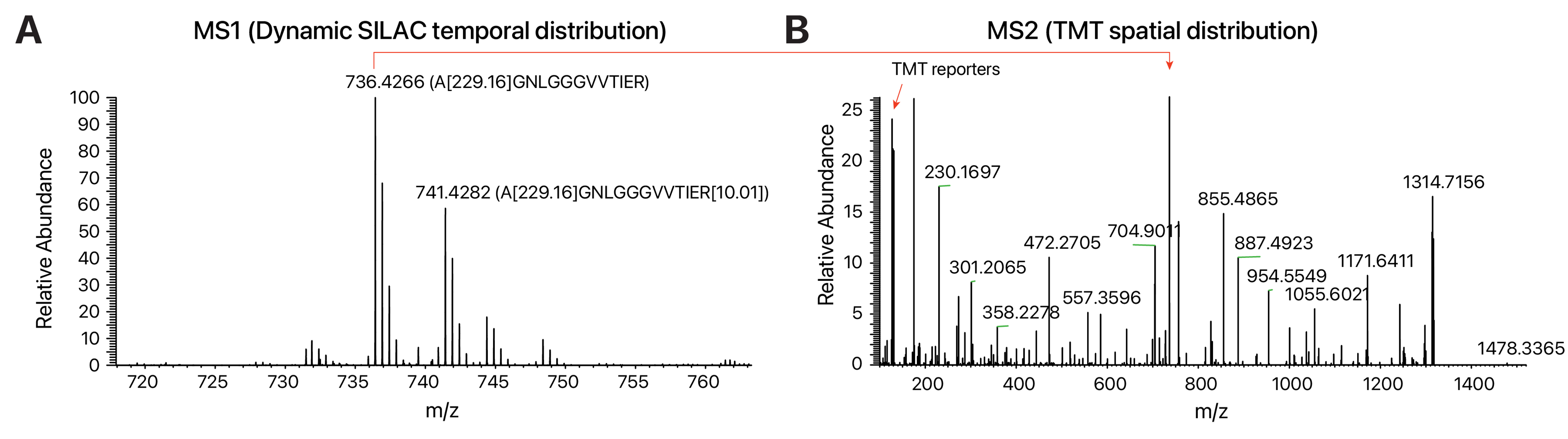
Figure 1. Example MS1 and MS2 spectra with protein turnover and spatial distribution information. Adapted from our previous data deposited to ProteomeXchange at PXD038054. (A) MS1 spectrum showing the light/heavy SILAC and TMT doubled-labeled peptide AGNLGGGVVTIER from large ribosomal subunit protein eL22 (RPL22). Approximately 35% of the peptide pool contains newly synthesized peptides (+10.0083 arginine) after 16 h of labeling. (B) Corresponding MS2 spectrum of the peptide from the same mass spectrometry experiments, showing fragment ions used for determining peptide sequences as well as the TMT reporters (red arrow to the left, m/z 126–131) that encode relative abundance of the peptide in each ultracentrifugation fraction. The fraction profile is then used in supervised or semi-supervised classification to determine the subcellular localization of the RPL22 protein.
Figure 2 shows the compartment classifications of one sample from a previously generated data set deposited to ProteomeXchange (normal AC16, replicate number 2; PXD046669). Figure 2A shows the T-distributed stochastic neighbor embedding (t-SNE) representation of the TAGM-MAP classification of proteins based on the TMT channel intensities. Figure 2B shows the distribution of proteins with TAGM MAP probability >95%, colored by the compartments to which they are assigned. In Figure 2C, pie charts show that classification can be verified by comparing the assigned compartments of non-marker proteins to their known UniProt annotations. Proteins that match the assigned compartment in the experiment are shown in green. The example protein from Figure 1, RPL22, is assigned to the ribosome fraction with high confidence (TAGM probability ~1), matching its existing UniProt annotation.
This protocol has been used and validated in the following research article:
• Currie et al. [14] Simultaneous proteome localization and turnover analysis reveals spatiotemporal features of protein homeostasis disruptions. Nature Communications.
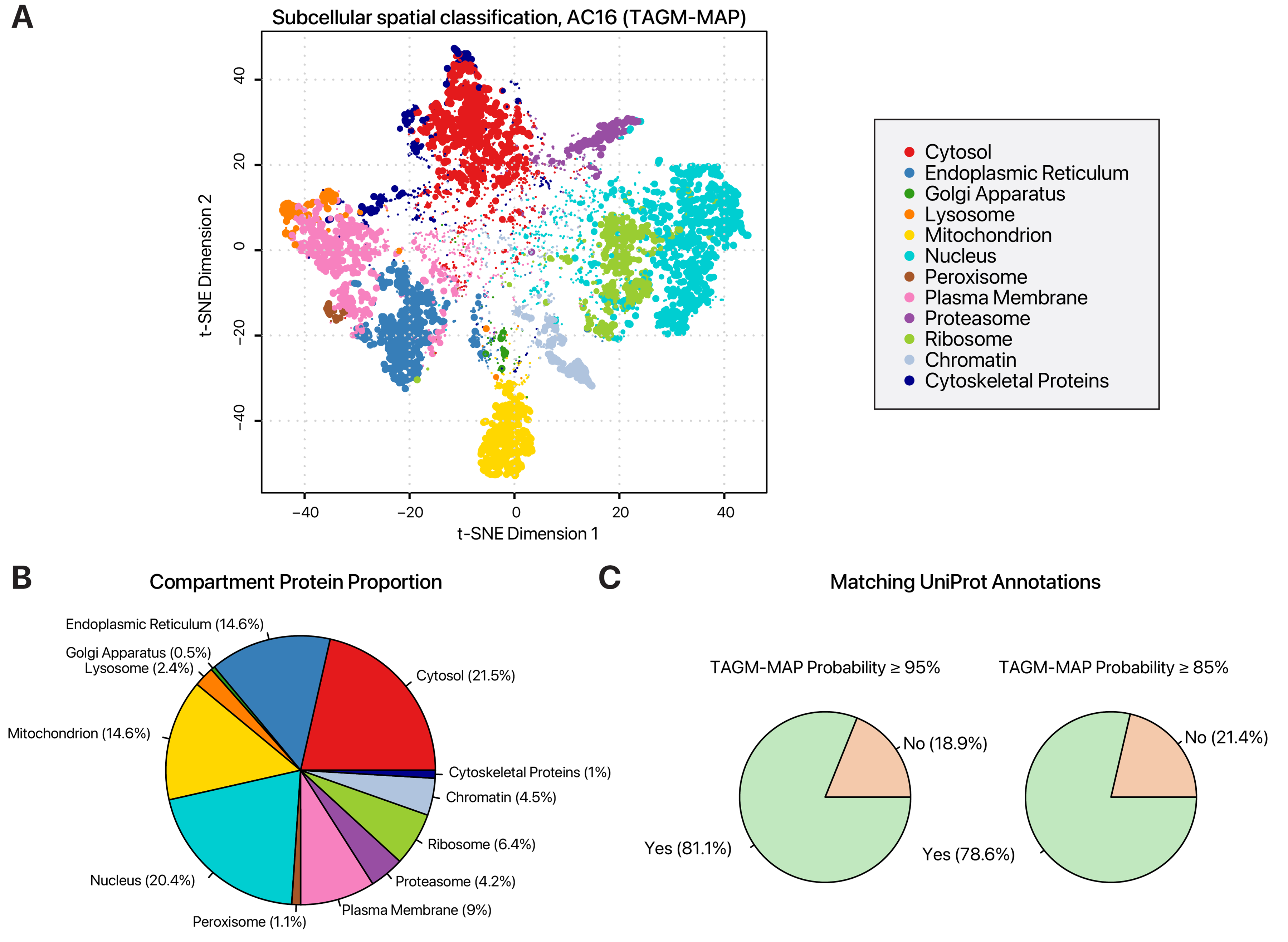
Figure 2. Typical subcellular localization distributions in human AC16 cells. (A) T-distributed stochastic neighbor embedding (t-SNE) plot of protein subcellular localization in human AC16 cells, classified using the TAGM-MAP method in pRoloc. Each data point represents a light or heavy SILAC-labeled protein. Color denotes assigned subcellular localization. Data point size scales with localization probability. (B) Pie chart showing the proportion of proteins assigned to each of 12 subcellular localizations. Colors correspond to the subcellular localizations as in panel (A). The cytosol, nucleus, and mitochondria contain the most assigned proteins. (C) Pie charts showing the proportion of assigned protein localizations with matching UniProt annotations at TAGM-MAP probability thresholds of 95% (left) or 85% (right). Comparison with existing annotations can be used to verify the spatial assignments.
General notes and troubleshooting
General notes
The cell culture, labeling, and fractionation steps of the protocol should be readily adopted in many cell biology and biochemistry laboratories. For laboratories that do not focus on mass spectrometry, we note that the mass spectrometry data acquisition steps of the protocol are compatible with common instrumentations in contemporary proteomics research and can be easily performed in institutional core facilities. The depth of the spatial proteomics analysis will depend on the performance of mass spectrometry and liquid chromatography separation, as well as the technical quality in cell lysis and ultracentrifugation. In prior work, the subcellular localization of 3,000–5,000 proteins could be confidently assigned. Each cell type is expected to have a different proteome as well as potentially cell type–specific protein localization; therefore, not every protein may match UniProt annotations. The marker proteins for training the TAGM-MAP (or other) classification model would need to be selected differently. In addition, some compartments may be apparent in some cell types but not others; hence, compartment labels may also need to be customized judiciously based on cell type and pilot data. Finally, it would be expected that some proteins (e.g., dually localized proteins or unknown compartments) would not have confidently assigned spatial profiles, even if the experiments were done correctly. Readers are referred to the latest spatial proteomics literature for ongoing advances [5].
The duration of SILAC labeling and collection timepoint(s) should be chosen based on prior knowledge of the average protein flux in the cell model, which is influenced by the doubling rate of proliferating cells. In addition, the timepoint(s) of interest may be chosen via prior knowledge of the timescale of the biological process of interest. Protein turnover rate constants can be confidently determined from as few as one collection time point, provided the protein has accumulated detectable SILAC labels but has not yet reached the plateau of the kinetic curve during the time of sample collection. However, a single-timepoint sampling approach would be disadvantaged in accuracy as well as the total span of measured turnover rates compared with a full time-series design.
The described protocol can be applied to different cell types. In prior work, we have applied it successfully to both transformed human AC16 cells as well as post-mitotic human induced pluripotent stem cell (hiPSC)-derived cardiomyocytes [14]. Other cell types that are compatible with both the dynamic SILAC and spatial proteomics components, including primary and pluripotent cells, may also be used. Both the spatial proteomics [15] and dynamic SILAC [16] components of this workflow can be applied to animal models. Hence, there is no theoretical barrier we are aware of for applying this method to in vivo models, although this has not been demonstrated and may require additional troubleshooting.
This protocol may be used to find differences in turnover rate constants of individual proteins across different subcellular locations. In previous work, we used it to find turnover differences in different compartments upon stimuli, e.g., in AC16 cells, the synthesis-degradation kinetics of ER-localized proteins is less repressed upon ER stress, when compared to proteins in other subcellular compartments [14]. In the same study, in hiPSC-derived cardiomyocytes exposed to the proteasome inhibitor carfilzomib, we found a preferential slowdown in the turnover of sarcomeric compartment proteins. Lastly, this protocol may also be used to compare localization changes (i.e., different assignment of compartments in different conditions) as in other spatial proteomics experiments. Moreover, as the MS2 spectra are generated separately for light and heavy SILAC-labeled peptides, this protocol may be used to find whether the light (existing) and heavy (synthesized post-labeling) proteins localize to different compartments, which may reflect trafficking and protein life cycle changes.
Troubleshooting
Problem 1: Low protein concentration after ultracentrifugation.
Possible cause: Insufficient number of strokes through the cell homogenizer.
Solution: Increase the number of strokes during homogenization of the cell lysate.
Problem 2: Acetone-precipitated pellets are difficult to resuspend.
Possible cause: Pellets were dried for longer than 30 min.
Solution: Resuspend the pellet immediately after acetone has evaporated or allow the pellet to sit in the resolubilization buffer for 1 h before resuspending.
Problem 3: Inadequate resolution between fractions to acquire subcellular localizations.
Possible cause: Supernatant was not completely removed from the pellet after ultracentrifugation steps.
Solution: Ensure the entire supernatant is removed from the pellet at each centrifugation step.
Problem 4: Organelle profiles are not sufficiently distinct from each other.
Possible cause: Markers are not ideal for the chosen cell line.
Solution: Use the acquired dataset to prune marker outliers and add proteins consistently localized to an organelle between conditions and replicates to the markers list.
Problem 5: Insufficient number of proteins identified.
Possible cause: Complexity of samples, especially with heavy SILAC-labeled peaks, requires more in-depth mass spectrometry analysis.
Solution: This may be achieved by increasing the number of offline first-dimension reverse-phase liquid chromatography (RP-LC) fractions or increasing the second-dimension gradient length and mass spectrometry data acquisition time.
Problem 6: Turnover between control and treatment is largely unchanged.
Possible cause: Data point collected did not align with cell line–specific protein turnover rate.
Solution: Optimize heavy media exposure to align with the average rate or protein half-life for the chosen cell line.
Acknowledgments
Conceptualization, M.P.L., E.L.; Writing—Original Draft, L.A., A.B.; Writing—Review & Editing, M.P.L., E.L.; Funding acquisition, M.P.L., E.L.; Supervision, M.P.L., E.L. This work was supported in part by NIH grants R35GM146815 to E.L.; NIH award R01HL169473 to E.L. and M.P.L.; and NIH awards R01GM144456 and R01HL141278 to M.P.L. The content is solely the responsibility of the authors and does not necessarily represent the official views of the National Institutes of Health. This protocol was used in [14].
Competing interests
The authors declare no conflicts of interest.
References
- Doherty, M. K., Hammond, D. E., Clague, M. J., Gaskell, S. J. and Beynon, R. J. (2008). Turnover of the Human Proteome: Determination of Protein Intracellular Stability by Dynamic SILAC. J Proteome Res. 8(1): 104–112. https://doi.org/10.1021/pr800641v
- Schwanhäusser, B., Busse, D., Li, N., Dittmar, G., Schuchhardt, J., Wolf, J., Chen, W. and Selbach, M. (2011). Global quantification of mammalian gene expression control. Nature. 473(7347): 337–342. https://doi.org/10.1038/nature10098
- Swovick, K., Firsanov, D., Welle, K. A., Hryhorenko, J. R., Wise, J. P., George, C., Sformo, T. L., Seluanov, A., Gorbunova, V., Ghaemmaghami, S., et al. (2021). Interspecies Differences in Proteome Turnover Kinetics Are Correlated With Life Spans and Energetic Demands. Mol Cell Proteomics. 20: 100041. https://doi.org/10.1074/mcp.ra120.002301
- Thul, P. J., Åkesson, L., Wiking, M., Mahdessian, D., Geladaki, A., Ait Blal, H., Alm, T., Asplund, A., Björk, L., Breckels, L. M., et al. (2017). A subcellular map of the human proteome. Science. 356(6340): eaal3321. https://doi.org/10.1126/science.aal3321
- Breckels, L. M., Hutchings, C., Ingole, K. D., Kim, S., Lilley, K. S., Makwana, M. V., McCaskie, K. J. and Villanueva, E. (2024). Advances in spatial proteomics: Mapping proteome architecture from protein complexes to subcellular localizations. Cell Chem Biol. 31(9): 1665–1687. https://doi.org/10.1016/j.chembiol.2024.08.008
- Foster, L. J., de Hoog, C. L., Zhang, Y., Zhang, Y., Xie, X., Mootha, V. K. and Mann, M. (2006). A Mammalian Organelle Map by Protein Correlation Profiling. Cell. 125(1): 187–199. https://doi.org/10.1016/j.cell.2006.03.022
- Geladaki, A., Kočevar Britovšek, N., Breckels, L. M., Smith, T. S., Vennard, O. L., Mulvey, C. M., Crook, O. M., Gatto, L. and Lilley, K. S. (2019). Combining LOPIT with differential ultracentrifugation for high-resolution spatial proteomics. Nat Commun. 10(1): 331. https://doi.org/10.1038/s41467-018-08191-w
- Dunkley, T., Watson, R., Griffin, J., Dupree, P. and Lilley, K. (2004). Localization of Organelle Proteins by Isotope Tagging (LOPIT). Mol Cell Proteomics. 3(11): 1128–1134. https://doi.org/10.1074/mcp.t400009-mcp200
- Mulvey, C. M., Breckels, L. M., Geladaki, A., Britovšek, N. K., Nightingale, D. J. H., Christoforou, A., Elzek, M., Deery, M. J., Gatto, L., Lilley, K. S., et al. (2017). Using hyperLOPIT to perform high-resolution mapping of the spatial proteome. Nat Protoc. 12(6): 1110–1135. https://doi.org/10.1038/nprot.2017.026
- Schessner, J. P., Albrecht, V., Davies, A. K., Sinitcyn, P. and Borner, G. H. H. (2023). Deep and fast label-free Dynamic Organellar Mapping. Nat Commun. 14(1): 5252. https://doi.org/10.1038/s41467-023-41000-7
- Itzhak, D. N., Tyanova, S., Cox, J. and Borner, G. H. (2016). Global, quantitative and dynamic mapping of protein subcellular localization. eLife. 5: e16950. https://doi.org/10.7554/elife.16950
- Kim, T. Y., Wang, D., Kim, A. K., Lau, E., Lin, A. J., Liem, D. A., Zhang, J., Zong, N. C., Lam, M. P., Ping, P., et al. (2012). Metabolic Labeling Reveals Proteome Dynamics of Mouse Mitochondria. Mol Cell Proteomics. 11(12): 1586–1594. https://doi.org/10.1074/mcp.m112.021162
- Yuan, F., Li, Y., Zhou, X., Meng, P. and Zou, P. (2023). Spatially resolved mapping of proteome turnover dynamics with subcellular precision. Nat Commun. 14(1): e1038/s41467–023–42861–8. https://doi.org/10.1038/s41467-023-42861-8
- Currie, J., Manda, V., Robinson, S. K., Lai, C., Agnihotri, V., Hidalgo, V., Ludwig, R. W., Zhang, K., Pavelka, J., Wang, Z. V., et al. (2024). Simultaneous proteome localization and turnover analysis reveals spatiotemporal features of protein homeostasis disruptions. Nat Commun. 15(1): 2207. https://doi.org/10.1038/s41467-024-46600-5
- Fang, H., Rai, A., Eslami, S. S., Huynh, K., Liao, H. C., Salim, A. and Greening, D. W. (2025). Proteomics and Machine Learning–Based Approach to Decipher Subcellular Proteome of Mouse Heart. Mol Cell Proteomics. 24(4): 100952. https://doi.org/10.1016/j.mcpro.2025.100952
- Hammond, D. E., Simpson, D. M., Franco, C., Muelas, M. W., Waters, J., Ludwig, R. W., Prescott, M. C., Hurst, J. L., Beynon, R. J., Lau, E., et al. (2021). Harmonizing labeling and analytical strategies to obtain protein turnover rates in intact adult animals. Mol Cell Proteomics. e472439. https://doi.org/10.1101/2021.12.13.472439
Article Information
Publication history
Received: Apr 28, 2025
Accepted: Jul 6, 2025
Available online: Jul 29, 2025
Published: Aug 5, 2025
Copyright
© 2025 The Author(s); This is an open access article under the CC BY-NC license (https://creativecommons.org/licenses/by-nc/4.0/).
How to cite
Alamillo, L., Black, A., Lam, M. P. Y. and Lau, E. (2025). Protein Turnover Dynamics Analysis With Subcellular Spatial Resolution. Bio-protocol 15(15): e5409. DOI: 10.21769/BioProtoc.5409.
Category
Systems Biology > Spatial transcriptomics
Biochemistry > Protein > Quantification
Cell Biology > Cell structure > Cell organelle
Do you have any questions about this protocol?
Post your question to gather feedback from the community. We will also invite the authors of this article to respond.