- Protocols

- Articles and Issues
- For Authors
- About
- Become a Reviewer

Method for Extracellular Electrochemical Impedance Spectroscopy on Epithelial Cell Monolayers
Published: Vol 15, Iss 12, Jun 20, 2025 DOI: 10.21769/BioProtoc.5341 Views: 3301
Reviewed by: Wendy Leanne HempstockAnonymous reviewer(s)
Advertisement


Protocol Collections
Comprehensive collections of detailed, peer-reviewed protocols focusing on specific topics


Related protocols

Abstract
Epithelial tissues form barriers to the flow of ions, nutrients, waste products, bacteria, and viruses. The conventional electrophysiology measurement of transepithelial resistance (TEER/TER) can quantify epithelial barrier integrity, but does not capture all the electrical behavior of the tissue or provide insight into membrane-specific properties. Electrochemical impedance spectroscopy, in addition to measurement of TER, enables measurement of transepithelial capacitance (TEC) and a ratio of electrical time constants for the tissue, which we term the membrane ratio. This protocol describes how to perform galvanostatic electrochemical impedance spectroscopy on epithelia using commercially available cell culture inserts and chambers, detailing the apparatus, electrical signal, fitting technique, and error quantification. The measurement can be performed in under 1 min on commercially available cell culture inserts and electrophysiology chambers using instrumentation capable of galvanostatic sinusoidal signal processing (4 μA amplitude, 2 Hz to 50 kHz). All fits to the model have less than 10 Ω mean absolute error, revealing repeatable values distinct for each cell type. On representative retinal pigment (n = 3) and bronchiolar epithelial samples (n = 4), TER measurements were 500–667 Ω·cm2 and 955–1,034 Ω·cm2 (within the expected range), TEC measurements were 3.65–4.10 μF/cm2 and 1.07–1.10 μF/cm2, and membrane ratio measurements were 18–22 and 1.9–2.2, respectively.
Key features
• This protocol requires preexisting experience with culturing epithelial cells (such as Caco-2, RPE, and 16HBE) for a successful outcome.
• Builds upon methods by Lewallen et al. [1] and Linz et al. [2], integrating commercial chambers and providing a quantitative estimate of error.
• Provides code to run measurement, process data, and report error; requires access to MATLAB software, but no coding experience is necessary.
• Allows for repeated measurements on the same sample.
Keywords: Electrochemical impedance spectroscopyGraphical overview
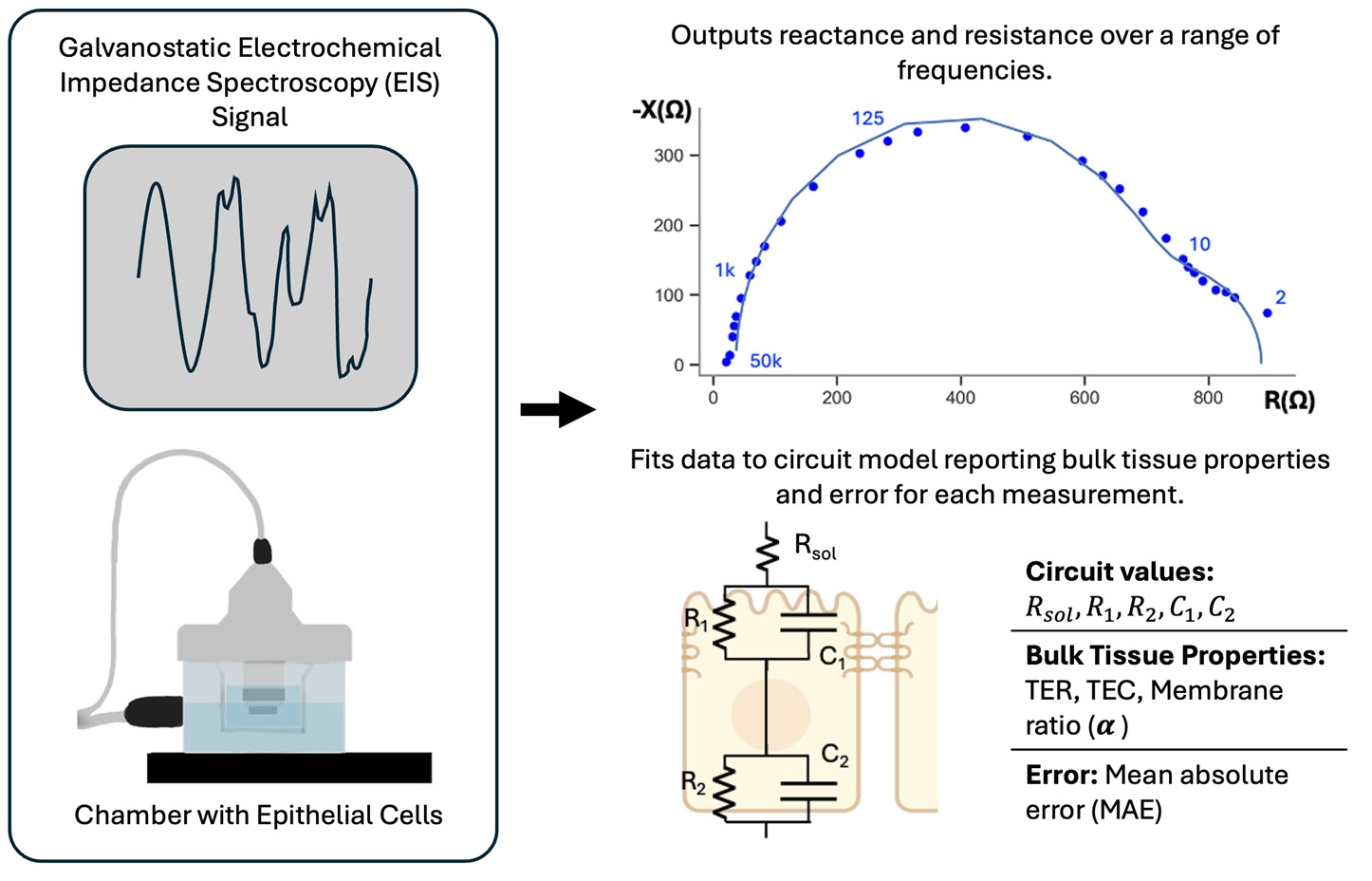
Electrochemical impedance spectroscopy measurement involves sending a galvanostatic signal through the electrophysiology chamber and across the epithelial cell monolayer (left) and results in complex impedance data at each frequency. This data is then fit to an electrical circuit model to output transepithelial resistance (TER), transepithelial capacitance (TEC), and membrane ratio (α) (right).
Background
Epithelial electrophysiology can provide insight into epithelial barrier function by measuring the electrical properties associated with the transport of ions, nutrients, and waste products [3,4]. Furthermore, transport across the tissue can be perturbed by blocking and activating ion channels or degrading tight junctions formed between the cells to isolate specific pathways or channels. This perturbation is useful for understanding healthy and diseased models, testing therapeutics, and characterizing quality control of in vitro cultures [1,5,6].
Transepithelial resistance (TER; also known as transepithelial electrical resistance, TEER) has become the gold standard over the last 30 years for quantifying epithelial tissue maturity and barrier integrity using commercial or custom electrodes and chambers [4,7,8]. Electrochemical impedance spectroscopy (EIS/ECIS), although not yet widely adopted, has been shown to offer insights into epithelial transport dynamics, membrane-specific properties, and more accurate measurements of membrane integrity. For example, Lewallen et al. showed the advantages of combining EIS with intracellular voltage recording to distinguish apical and basolateral transport function during adenosine triphosphate administration [1] in a custom Ussing chamber and automated electrode placement [9]. Cottrill et al. reported similar parameters without intracellular voltage recording, by making assumptions about relative permeability [10]. Linz et al. integrated EIS into existing commercial electrodes (STX, World Precision Instruments) to measure Caco-2 monolayer dynamics in response to stimuli: saponin, sonoporation, and calcium chelator ethyleneglycol-bis(beta-aminoethyl ether)-N, N’-tetraacetic acid (EGTA) [2].
Transepithelial resistance (TER) is a good indicator of tight junction development and membrane integrity. Tight junctions form between the cells, creating a paracellular pathway as shown in Figure 1A. The electrical resistance of the tissue is dominated, but not determined exclusively, by this paracellular pathway, compared to the flow of ions through the respective apical and basolateral membranes [11–13].
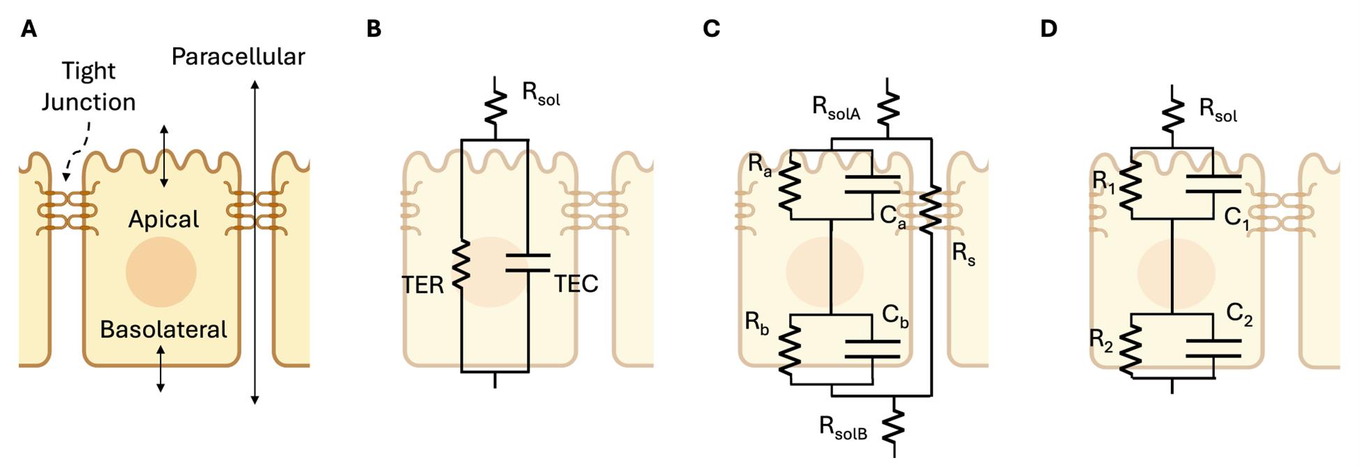
Figure 1. Circuit models for transport across an epithelial monolayer. Modified from Lewallen et al. [1]. (A) Physical model: cross-section schematic of an epithelial tissue showing the three pathways where transport is regulated: apical, basolateral, and paracellular pathways. (B) Three-parameter circuit model: a simple resistor-capacitor (RC) circuit that can be fit from extracellular electrodes alone, widely used to measure transepithelial resistance (TER) and transepithelial capacitance (TEC) despite its low fidelity. (C) Seven-parameter model with apical, basolateral, and paracellular pathways requires intracellular voltage measurement to fully solve [1,14]. (D) Five-parameter model, which we refer to as the RCRC model, with two resistors (R) and 2 capacitors (C) representing the cell layer, shown to model the apical and basolateral cell membranes of Caco-2 cells in Linz et al. [2].
TER measurement is typically performed at a single frequency (e.g., 12.5 or 75 Hz [7,15]), assuming resistance is independent of frequency (i.e., reactance is negligible). Yet, it has been observed that reactance is not negligible [1,2,16] and therefore, this assumption is not valid. As a result, the TER measured with a single frequency is erroneously low. For example, bronchiolar epithelia show a strong frequency-dependent change in resistance (see Figure 2). Mathematical models of epithelia that include reactance contributed by capacitance, as shown in Figure 1B–D, can more accurately fit the measurements across frequencies. Figure 2 shows an EIS data fit with the model from Figure 1D. In this figure, called a Nyquist plot, the resistance (R) and reactance (X) are the real and imaginary components of the complex impedance (Z), measured as a function of frequency.
Adding capacitive elements to the model (Figure 1B–D) can yield novel insights about the epithelial barrier. EIS measurements of TER from fitting a circuit model, as shown in Figure 2, inherently separate the electrical resistance of the tissue from the transwell and media, termed Rsolution, shortened to Rsol. Thus, unlike traditional TER measurement, “background subtraction” from a blank is not necessary. The impedance measurements also capture capacitance, enabling one to model charge blockage or storage at the tissue surface, a frequency-dependent property [1,2,16]. In addition, transepithelial capacitance (TEC) shows promise in describing cell properties such as cell volume or surface area [17–20]. Although cell capacitance has been used for single cells to identify cell types in cytometry, rigorous biological studies have yet to be published correlating the TEC of a monolayer of cells to a specific cell property.
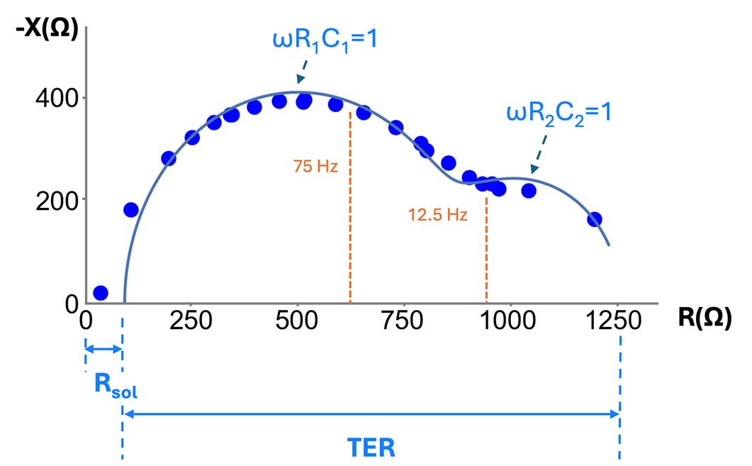
Figure 2. Nyquist plot of negative reactance (-X) vs. resistance (R) for frequencies of 2 Hz to 10 kHz on a measurement of bronchiolar epithelia (at day 7). Each point is the measured reactance and resistance for a given frequency; all measurements were taken on a single sample. TER measurements taken at a single frequency, such as 12.5 Hz and 75 Hz and shown in orange, underestimate TER [21] and require background subtraction. Each capacitance component can be estimated based on the approximate peak of each semicircular curve in the Nyquist plot, where at the peak, .
Figure 1B shows the simplest model that accounts for capacitance and lumps the apical and basal membrane, along with the paracellular properties, into single values of TER and TEC. While insightful and implemented in commercial devices (CellZscope, NanoAnalytics), we have shown that some epithelial tissues, like bronchiolar epithelia, require more detailed models to accurately calculate TER (e.g., Figure 1C, D [22]). Figure 1C, while modeling the apical, basolateral, and paracellular pathways separately, requires intracellular measurement to solve [1]; thus, the method we present here relies on the model of Figure 1D. This model can capture the different time constants observed in the data (τ = RC), yet can be measured with only extracellular electrodes. This model has been used in prior publications to analyze impedance data on Caco-2 cells changing in response to forskolin [2]. However, one of the shortcomings of the model of Figure 1D is that the paracellular resistance is lumped into R1, R2, C1, C2 and is therefore not resolvable.
With off-the-shelf electronic circuitry and software, we have developed a method for fitting an electronic model to measure the resistances and time constants associated with tissue changes. The cells are grown on the same transwells and tested in the same chambers used for conventional TER measurement. The electronic circuitry performs galvanostatic signal processing (e.g., analog to digital conversion, modulation) and conversion to impedance. The custom software performs mathematical and data analysis (e.g., fitting and error calculation). The electrical current is set to less than 10 μA to maintain linearity [16,20], and the frequency sweep is chosen such that the reactance is approximately zero at the bounds of the range, or approximately 2 Hz–50 kHz, with frequencies logarithmically spaced. We take these impedance measurements on retinal pigment epithelia (RPE) and bronchiolar epithelia (16HBE), and report transepithelial resistance (TER), transepithelial capacitance (TEC), membrane ratio (α), and a validated metric of reporting measurement error, the mean absolute error (MAE).
Prior to describing the method for epithelia, we will first discuss our validation of the EIS and fitting technique on electrical circuits that mimic the TER and TEC of living tissues. We soldered circuits with commonly observed TER and TEC values of mature tissues and lower TER and TEC values representing developing tissues, resulting in four electrical circuits: 16HBE1, 16HBE2, RPE1, and RPE2, as shown in Figure 3. The results show precise and accurate TER (< 7 Ω error, < 1 Ω SD), TEC [< 0.12 μF error (< 0.025 μF SD)], Rsol [< 4 Ω error (< 0.4 Ω SD)], and membrane ratio < 1.5 error (< 0.6 SD) for all four circuit models. Individual circuit parameters Rsol, R1, R2, C1, C2, and their errors are reported in Figure S2.
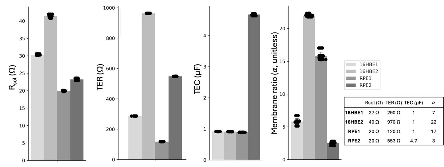
Figure 3. Electrochemical impedance spectroscopy (EIS) measurement and fitting to the RCRC model (Figure 1D) on four electrical circuits (16HBE1, 16HBE2, RPE1, RPE2) simulating bronchiolar epithelia (16HBE) and retinal pigment epithelia (RPE) cell layers. Six replicate EIS measurements were taken on each circuit, and all six measurements were fit six times to include fitting variability. Transepithelial resistance (TER) (< 7 Ω error, < 1 Ω SD), transepithelial capacitance (TEC) [< 0.12 μF error (< 0.025 μF SD)], Rsol [< 4 Ω error (< 0.4 Ω SD)], and membrane ratio < 1.5 error (< 0.6 SD) for all four circuit models. Signal 2 Hz–50 kHz, 2 freq/dec, 4 μA. Table inset: actual circuit values.
Materials and reagents
Biological materials
1. 16HBE14o, human bronchiolar epithelial cells (Millipore Sigma, catalog number: SCC150) grown to confluency: 7 days after seeding at 250k cells/12-well transwell in 12 mm Transwell® with 0.4 μm pore PET membrane insert [23]
2. iPSC-derived retinal pigment epithelia grown to maturity (Sharma et al. [24,25]) in 12 mm Transwell® with 0.4 μm pore PET membrane insert
Reagents
1. RPE cell culture media (Sharma et al. [24])
a. 90% MEM alpha (Thermo Fisher, catalog number: 12571063)
b. 5% fetal bovine serum, heat inactivated (Hyclone, catalog number: SH30071.03)
c. 1% N-2 supplement (Life Technologies, catalog number: 17502048)
d. 1% penicillin-streptomycin (Life Technologies, catalog number: 15140-148)
e. 1 mM sodium pyruvate (Life Technologies, catalog number: 11360-070)
f. 0.1 mM MEM non-essential amino acids (Life Technologies, catalog number: 11140)
g. 250 μg/mL taurine (Sigma, catalog number: T0625)
h. 20 μg/L hydrocortisone (Sigma, catalog number: H6909)
i. 0.013 μg/L 3,3’,5-Triiodo-L-thyronine (T3) (Sigma, catalog number: T5516)
2. 16HBE culture media (concentrations based on the medium used by the Cystic Fibrosis Foundation [26])
a. 89% MEM media (Thermo Fisher Scientific, catalog number: 11095098)
b. 10% fetal bovine serum, premium, heat inactivated (R&D Systems, catalog number: S11150H)
c. 1% penicillin-streptomycin (5,000 U/mL) (Thermo Fisher Scientific, catalog number: 15070063)
3. Reagent-grade alcohol (VWR, catalog number: BDH1164-4LP)
4. Deionized water (e.g., Millipore Milli-Q Water Purification System)
5. Sodium hypochlorite, 5% w/v (LabChem, catalog number: 1310-73-2)
Laboratory supplies
Biological supplies
1. 1× 12 mm Transwell® with 0.4 μm pore PET membrane insert with no cells seeded (Corning, catalog number: 3460)
2. Spray bottle (Fisher Scientific, catalog number: 02-991-721)
3. 2× 50 mL Falcon tube (Corning, catalog number: 352070)
4. Lint-free wipes (Kimtech Science, catalog number: 34120)
5. P1000 pipette (VWR, catalog number: 83009-776)
6. P1000 tips (VWR, catalog number: 76322-154)
7. Sterile forceps (VWR, catalog number: 82027-408)
Electrical supplies
1. EndOhm (12 mm) (World Precision Instruments, catalog number: EndOhm-12G)
2. EndOhm to RJ11 cable (World Precision Instruments, catalog number: 53330-01)
3. USB-C to USB-A adapter (j5Create, catalog number: JCD383)
4. Parts for RJ11 to banana adapter:
a. 5× banana plug (Digikey, catalog number: J356-ND)
b. RJ11 female connector (Amazon Uxcell, catalog number: B01HU7BX42)
c. Plastic housing box (P200 tip box) (VWR, catalog number: 76322-150)
d. M12 drill bit (Drill America, catalog number: POUM12X1.25)
e. Solder (Digikey, catalog number: SMDIN52SN48-ND)
f. Superglue (Loctite, catalog number: 1799408)
Equipment
1. Multi Autolab cabinet for M204 modules (Metrohm, catalog number: AUT.MAC204.S)
a. M204 multichannel PGSTAT module (Metrohm, catalog number: AUTM204.S)
b. FRA32M module for M101/204/PGSTAT204 (Metrohm, catalog number: FRA32M.MAC.204.S)
c. Autolab banana cable (Metrohm)
d. Autolab power cable (Metrohm)
e. USB-A to USB-B 2.0 cable (Metrohm)
f. Autolab test cell (Metrohm, catalog number: 3500002470)
2. PC with CPU 1 GHz or faster 64-bit processor, 2 GB RAM, 20 GB hard space, DirectX 9.0c compliant display adaptor with 64 MB RAM [Dell laptop, CPU intel i9 core, 2.50 GHz, 64 GB RAM, 1.84 TB Hard drive, intel(R) UHD graphics GPU]
3. Laminar flow hood/biological safety cabinet (Labconco, model: Logic+ Type A2 Biosafety Cabinet)
4. Soldering iron (Digikey, catalog number: PES51-ND)
5. Drill (Dewalt, catalog number: DCD793B)
6. Multimeter with continuity feature (Fluke, catalog number: FLUKE-177 ESFP)
Software and datasets
1. MATLAB (Mathworks, 2024b)
2. Microsoft Excel (Microsoft, Version 16.92)
3. NOVA 2.1 (Metrohm, 2024)
4. Impedance Analysis GitHub (extracellularEIS, https://github.com/chien0507/extracellularEIS/tree/main)
a. Matlab Impedance Fitting Code (Nova_batch_20240125.m, Nova_function_20240125.m, fitZ12_20240125.m, funRCRC.m, makeTissueID.m)
b. NOVA Custom Galvanostatic EIS Protocol (protocol.nox)
Procedure
An overview of the procedure with estimates of how long it takes to complete each step is shown in Figure 4.
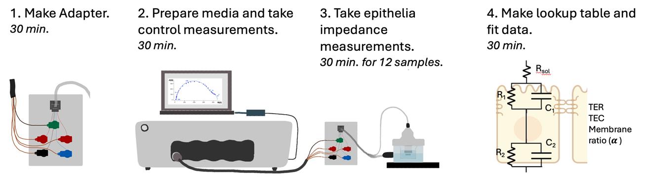
Figure 4. Procedure overview to measure extracellular electrochemical impedance spectroscopy on epithelial cell monolayers. Estimates of how long it takes to complete each step are italicized.
A. Fabricate adapter
1. Fabricate the RJ11 to banana adapter according to Figure 5 as follows: using the drill and drill bit, drill holes into the top of the plastic housing box, taking care not to crack the housing, for the five banana plugs (labeled GND, WE, S, CE, and RE). Insert plugs and secure them using the associated metal nuts. Also, drill one hole for the RJ11 adapter and glue it in place with superglue. Solder each wire on the RJ11 female connector to a metal tab on the back of a banana plug; there should be one banana plug that is not soldered to anything that serves as our floating ground (GND). The black wire from the female RJ11 adaptor is the sense pin, the green is the counter pin, the yellow is the working pin, and the red is the reference pin. Connect the EndOhm to the RJ11 to banana adapter. Check connections using the multimeter continuity feature by touching one probe to the banana plug in question and the other probe to each of the corresponding EndOhm electrodes labeled in Figure 5. Label the banana plugs accordingly (RE for reference, S for sense, CE for counter, WE for working). See Figure S1 for additional reference images.
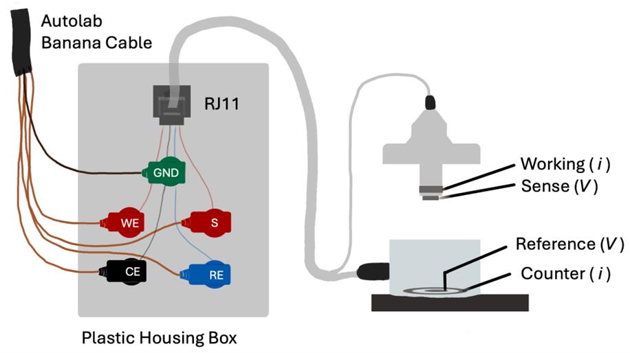
Figure 5. The RJ11 to banana adapter enables one to connect the Autolab M204 to the EndOhm. While performing the EIS measurement, the electrical current is sent across the working and counter electrodes, and the resulting voltage is measured across the reference and sense electrodes.
B. Experimental setup
1. Fill the spray bottle with reagent-grade alcohol.
2. Fill a 50 mL Falcon tube with ~20 mL of alcohol and place the forceps tips in the alcohol. Close the top and shake gently to sterilize the entire forceps. Place the Falcon tube into a sanitized laminar flow hood for transferring the cell culture inserts later.
3. In the laminar flow hood, transfer 5 mL of media (specific to the cell line that is being used) to the remaining Falcon tube using the P1000 pipette and tips. Wait for 10 min for the temperature of the media in the Falcon tube to reach room temperature.
C. Control impedance measurements
This section describes how to take control measurements on the Autolab test cell and on a blank transwell to ensure the system is connected and working properly prior to starting biological measurements. When measuring on the blank transwell and for all measurements on epithelia, the system will be set up as shown in Figure 6.
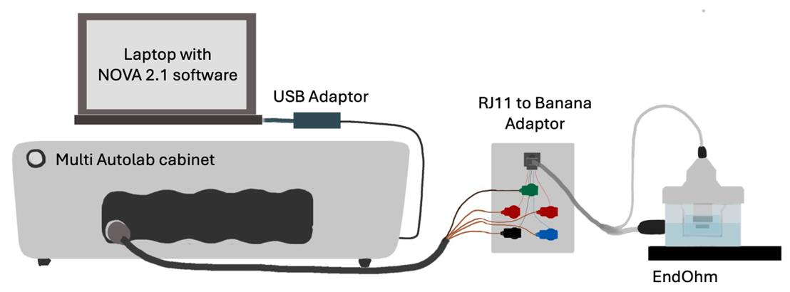
Figure 6. Diagram of instrument connections for extracellular impedance spectroscopy. The Multi Autolab cabinet (galvanostat) is connected to a chamber containing a transwell and electrodes for measurement.
1. Spray two lint-free wipes with reagent alcohol and put them inside the flow hood. Sterilize the EndOhm by spraying both the interior and exterior of the EndOhm generously with reagent alcohol before setting it to dry on the lint-free wipes for at least 10 min.
2. While waiting for the EndOhm to dry, plug the following into the Multi Autolab cabinet: Autolab banana cable, USB-A to USB-B 2.0 cable, and power cable connected to a wall outlet. Turn on the Multi Autolab cabinet. Connect the USB-B 2.0 to the PC (using the USB-C to USB-A adapter if necessary).
3. Connect the Autolab banana cable to the Autolab test cell, matching up the cable ends as shown in Figure 7(left). This connects the Autolab through the test cell’s 1 kΩ and 1 μF parallel RC circuit.
4. On the PC, open the NOVA software, open the GitHub link, and download the repository by clicking the green code button and Download ZIP. Find the downloaded zip folder in File Explorer and double-click the compressed file. Then, select extract all to unzip the file. The NOVA procedure to use is in the unzipped file, titled “protocol.nox.”
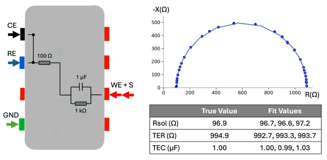
Figure 7. Model cell connections and measurements. Three EIS measurements on test cell, 2 Hz–50 kHz sweep, 2freq/dec, 5sines, and connections to the test cell are shown on the left; Nyquist plot with raw data and fit lines is shown on the right. Measurements and fit lines are indistinguishable between the three measurements; solution resistance and TER within 5 Ω, TEC within 0.03 μF.
5. In the NOVA software home screen, click Import Procedure and open the “protocol.nox.” file. The protocol sends a galvanostatic signal at 4 μA with two frequencies per decade, 1 s wait time before starting the measurement, and 5 frequencies stacked at low frequencies (5 sines). If more datapoints are desired for each sweep, you can increase the frequencies per decade.
6. As shown in Figure 8, in the opened protocol, select the Repeat n times block, then select the FRA measurement block, and finally the Freq Export block.
7. In the properties side panel that opens, enter the filename including the file path. For the file path, we recommend naming the file in the form “mediaUsed_TW1_day1_exp1_freq" but any filename without spaces will work. Impedance data is exported as a tab-delimited text file. This protocol outputs the resistance and reactance (real and imaginary impedance) for each frequency and the transepithelial voltage measured just before each frequency sweep.
8. On the NOVA software, start the measurement by clicking Measurement in the top menu, Run on, and then the channel the test cell is plugged into. A warning will pop up saying “current range (10 μA) is not sufficient for selected frequency (50,000 Hz)." Click OK. Once the measurement begins, the software switches to a new open tab on the left with the collected data. The Nyquist plot should appear in the bottom row of plots. Verify that the Nyquist plot generated resembles the shape shown in Figure 7. This data will be analyzed later to verify that the model cell resistance and capacitance are accurately measured. Data will automatically be exported at the end of the measurement. Close the data tab.
9. Disconnect the M204 banana cables from the test cell and connect them to the EndOhm using the RJ11 to banana adapter. Spray and wipe down the EndOhm to RJ11 cable before bringing the EndOhm end into the laminar flow hood and connecting to the EndOhm, as shown in Figure 5. The adapter and M204 remain outside of the flow hood, so temporarily taping EndOhm to RJ11 cable to the edge of the laminar flow hood prevents excess strain on the cable.
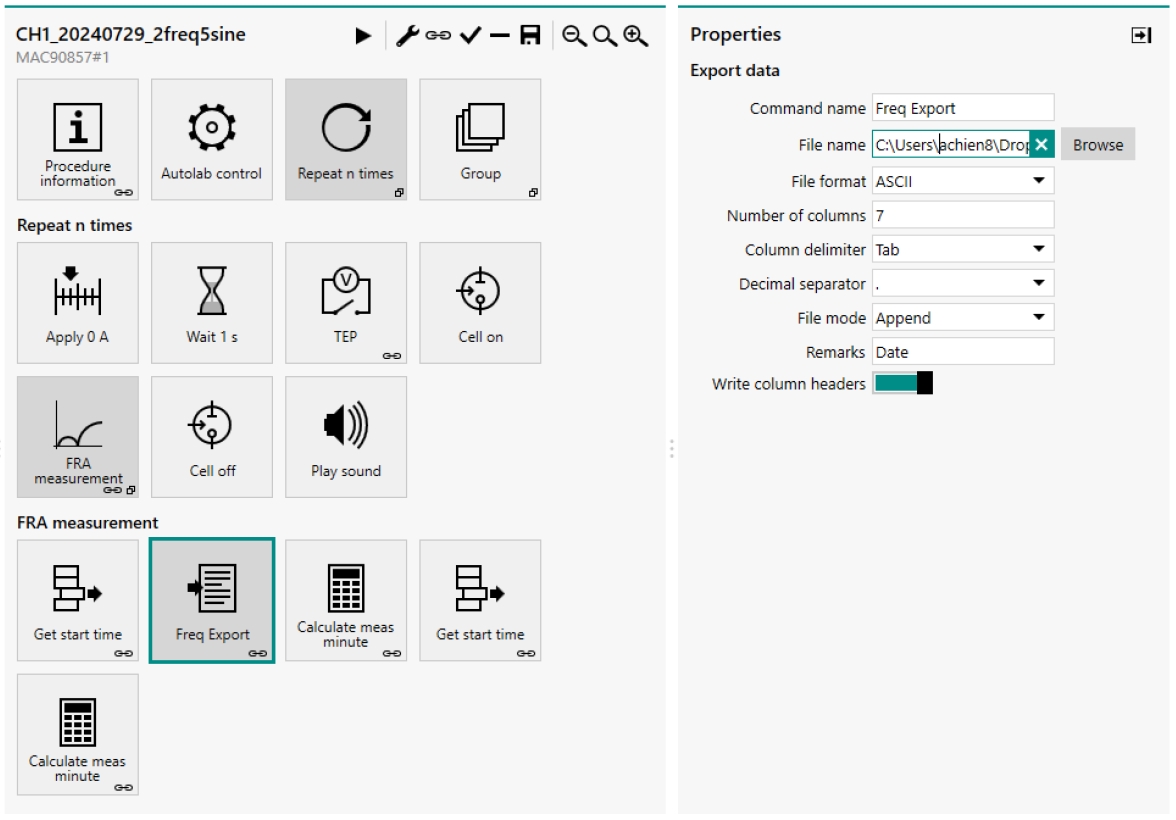
Figure 8. NOVA protocol. Screenshot showing how to change the file name on the right panel through the frequency export block.
10. Next, we will measure the impedance of a blank transwell to verify that its electrical properties are accurately measured. Depending on which cells will be measured in subsequent steps, add 2.5 mL of the corresponding cell culture media to the EndOhm using the P1000 pipette and tips. Avoid introducing bubbles by pipetting slowly.
11. In the laminar flow hood, take out the sterile forceps in reagent alcohol and shake lightly to dry off. Using the forceps, place the blank or empty cell culture insert into the EndOhm bottom. To prevent air bubbles from getting trapped on the bottom of the cell culture insert surface, contact the media surface at an angle before placing it level and releasing. Bubbles can be dislodged by lightly shaking the cell culture insert in the media solution or by removing and replacing it. See Figure 9 for what bubbles may look like on the bottom of the cell culture insert. See Troubleshooting problem 1 for more tips.
12. Pipette 700 μL of media into the apical side of the cell culture insert and place the EndOhm cap on top, once again lowering one edge first to prevent bubbles. If bubbles are present, they may affect impedance measurements. See Troubleshooting problem 1 for tips to remove bubbles. Examples of bubbles present on an EndOhm electrode are shown in Figure 9.
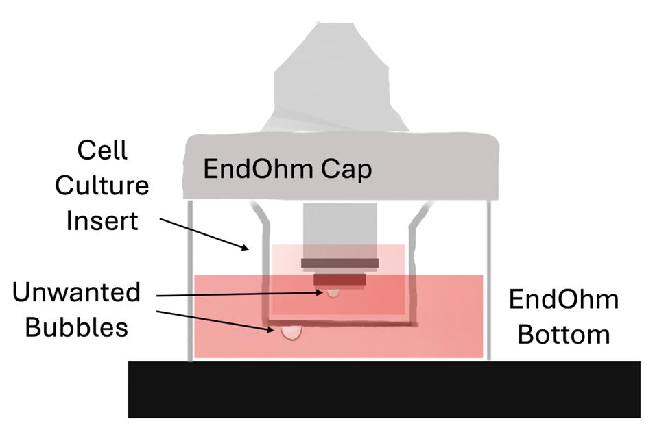
Figure 9. Bubbles in the EndOhm chamber. Bubbles easily form on the apical electrode surface and the cell culture insert bottom surface upon submersion, affecting impedance measurement accuracy. They should be prevented or removed as described in the procedure.
13. Change the file name and file path in the NOVA protocol again to reference the blank cell culture insert, as described in steps C6 and C7 and shown in Figure 8. Do not use a file name with spaces.
14. Run measurement as in step C8 on the blank cell culture insert. Also, note that the reactance should be distributed around a mean of zero as shown in Figure 10A. If the Nyquist plot shows a nearly vertical line, then the electrodes are not properly submerged in media, the cable is not connected, or the device is not running on the correct channel (see Figure 10B). This blank measurement is not necessary for every experiment but is useful to check whether the system is connected and working properly. Notably, bubbles will result in a larger scatter of real and imaginary impedances (Figure 10A).
15. Remove the blank cell culture insert and close the data tab.
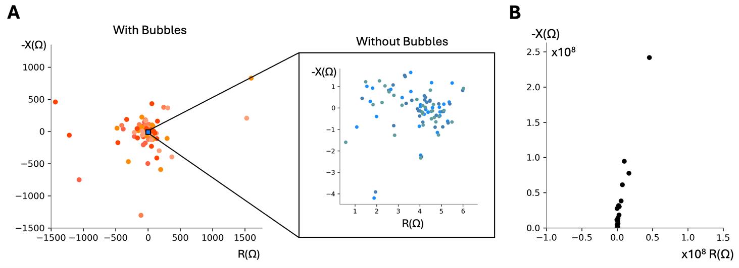
Figure 10. Nyquist plots of control blank measurements. (A) Nyquist plots of a blank cell culture insert with and without bubbles present. Six representative noisy blank cell culture insert measurements due to bubbles, each plotted in a different warm color, showing higher magnitude scatter (Corning 3460 transwell in RPE media) (left). Three representative blank cell culture insert measurements without bubbles (right). All points remain within ± 50 Ω resistance and negative reactance for good measurements. Resistances can vary across inserts. We have observed resistance values clustered around a value from 0 to 50 Ω resistance and 0 Ω reactance. Note: We have set a threshold in the fitting code to switch to fitting only to a resistor (no capacitance) determined experimentally when the Nyquist plots look like this, determined experimentally when neither of the following statements are no longer true: the minimum reactance is less than three times the median reactance value measured for blank transwells and the sum of the R1 and R2 values calculated is greater than 9. (B) Nyquist plot when apical electrodes are not submerged in apical solution, resulting in resistance and reactance values on the order of 108 Ω and a shape resembling a slanted line. Frequency sweep 2 Hz–50 kHz, 2freq/dec, 4 μA current.
D. Epithelia impedance measurements
1. Begin epithelia impedance measurement either by continuing from the preceding steps C1–15 in order or by following section B and then steps C1, C2, C4–5, and C9. The instrumentation should be connected as shown in Figure 6.
2. Obtain confluent cells on cell culture inserts following the protocols in [26] for bronchiolar or [24] for retinal epithelia.
3. Transfer cells from the incubator to the laminar flow hood and allow them to temperature stabilize for 5 min (within their existing well plate) before beginning measurement.
4. While the cells are cooling, add 2.5 mL of the corresponding cell culture media to the EndOhm gently using the P1000 pipette and tips to avoid introducing bubbles.
5. Take out the sterile forceps stored in reagent alcohol and shake them lightly to dry off. Using the forceps, place the culture insert into the EndOhm bottom.
6. Place the EndOhm cap on top, lowering one edge first to prevent bubbles. If bubbles are present, like those shown in Figure 9, they may affect impedance measurements. See Troubleshooting problem 1 for tips to remove bubbles.
7. Change the file path and file name in the NOVA protocol to reference the cell culture insert as in steps C6 and C7 (Figure 8), and run measurement on the cell culture insert as in step C8. If the cells have grown confluent, the Nyquist plot should look like a semicircle or two adjacent, intersecting semicircles . Representative examples of the Nyquist plot of bronchiolar epithelia are shown in Figure 11A, showing the two semicircles intersecting; retinal pigment epithelia are shown in Figure 11B.
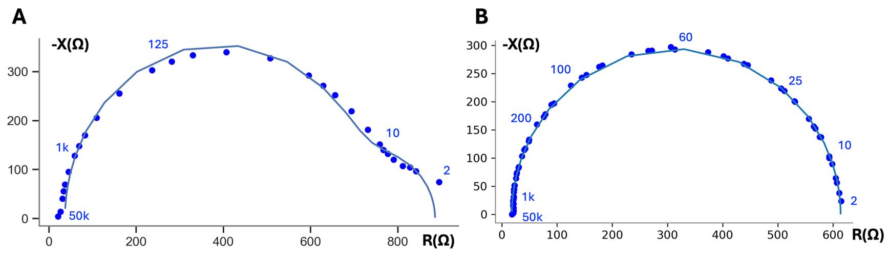
Figure 11. Representative Nyquist plot of 16HBE at day 7 (A) and mature RPE data (B) with frequency labels in blue, showing experimental data and fit line. Fit values normalized to 1.12 cm2 cross-sectional area: TER 950 Ω·cm2, TEC 1.06 μF/cm2. Representative Nyquist plot of RPE (A), showing experimental data and fit line. Fit values normalized to 1.12 cm2 cross-sectional area: TER 667 Ω·cm2, TEC 4.10 μF/cm2.
8. Once the measurement is complete, take the cell culture insert out of the EndOhm and replace with the next sample from the well plate. Basal media can remain in the EndOhm for all measurements on the same cell replicates. All measurements from a single 12-well plate can be completed in 30 min.
9. When all measurements are complete, return cells to the incubator in their original well plate. Rinse EndOhm top and bottom with deionized water to remove proteins and charged particles from the surface of the electrodes and let it dry on the benchtop.
Data analysis
In this section, we describe how to analyze complex impedance data to yield biological properties of interest: transepithelial resistance (TER), transepithelial capacitance (TEC), and membrane ratio. Specifically, we use a nonlinear least squares fitting algorithm, an established technique for fitting EIS data [27], to fit the impedance data collected in the preceding steps to the RCRC model in Figure 1D.
Several algorithms and steps are necessary to perform this analysis. For context, we first describe mathematically how this analysis is performed and then discuss how to quantify the error.
A. Mathematical model for experimental fit
Transepithelial impedance is complex and can be represented as the sum of two orthogonal values: resistance or real impedance, R(ω), and reactance or imaginary impedance, X(ω), where ω = 2πf, and f is the frequency in Hz, as shown in Figures 10 and 11. This complex impedance, Z(ω), can be expressed as
(1)
The measured complex impedance, Z, in Equation 1, can be mathematically modeled by combining the circuit elements in Figure 1D such that
(2)
where Z1 is the impedance from the first parallel resistor-capacitor circuit, and Z2 is the second, as shown below.
(3)
(4)
Note that Z' is complex and can be separated into its real (resistive) and imaginary (reactive) components in a similar form to Equation 1:
(5)
where
(6)
and
(7)
To relate Z' (model) to Z (measurement), we then use a nonlinear least squares solver to minimize an objective function, J, which is defined as the sum of the squared residuals, or error, between the measured and modeled data at all frequencies. J is calculated as
(8)
Where ωi represents each frequency. The values for Rsol, R1, R2, C1, and C2 that minimize the error are defined as the fit values.
In practice, we used MATLAB’s nonlinear least squares solver to minimize J (Eq. 8). Specifically, we use the function lsqcurvefit using code modified from Lewallen et al. [1] with the settings described in Table 1.
Table 1. Settings for nonlinear least squares fit. These non-default settings are configured in MATLAB’s optimoptions function and are applied to the lsqcurvefit algorithm.
| Parameter | Value | Description |
| MaxIterations | 3 × 10³ | Maximum sets of parameter values (Rs, R1, R2, C1, C2) tried before reporting the best. |
| MaxFunctionEvaluations | 3 × 10³ | Maximum number of function evaluations allowed. |
| FunctionTolerance | 3 × 10⁻⁹ | Tolerance for convergence based on the function value. |
| OptimalityTolerance | 5 × 10⁻⁷ | Tolerance for convergence based on the gradient of the error function. |
| StepTolerance | 1 × 10⁻⁹ | Tolerance for convergence based on the step size of the error function. |
To mitigate the risk of converging to local minima or boundary values, each fitting procedure was initialized with a grid of three initial guesses per parameter. Resistance and capacitance values are limited to spanning the ranges of previously reported membrane properties in epithelial tissues [1,2,20,22,28–31] and adjusted based on observation:
• C1, C2 [1 × 10⁻⁸, 1 × 10⁻⁴] F/cm2
• R1, R2 [0, 5000] Ω·cm2
• Rsol [0, 1000] Ω·cm2
Following the minimization of the objective function J, the TER can be computed. TER is measured as the series combination of R1 and R2, then normalized by the cross-sectional area.
where A is the cross-sectional area of the tissue in cm2, and TEC is computed as the series combination of C1 and C2, also normalized to area:
We also report the membrane ratio α as previously defined in Lewallen et al. [1]. For this circuit model, we define it as the ratio of the time constants of the two resistor-capacitor circuits as
B. Data normalization
Prior to fitting, we logarithmically scale and normalize the circuit element values, due to their significant difference in magnitude. This operation is reversed after fitting and is done to ensure that the fitting algorithm assigns similar weight to the relative error of each parameter.
Specifically, two different normalizations are performed during each fit: (1) the magnitude of each circuit element, Rsol, R1, R2, C1, and C2, is converted to a log (base 10) domain, and (2) the real impedance and imaginary impedance are normalized to their respective maximum values. Impedance values were normalized by dividing each resistance value by its maximum resistance magnitude for that sweep and dividing each reactance value by its maximum reactance magnitude for that sweep, such that the real and imaginary impedance all spanned the range of [-1, 1].
C. Error quantification
Aside from the application in cell electrophysiology, electrochemical impedance spectroscopy (EIS) is an established technique for studying electrode degradation and measuring battery properties. However, there are no well-established metrics for quantifying error in fitting EIS data, and no studies on quantifying error for biological EIS data.
In the past, we used the L2 norm of the residual (resnorm) [1] as a reasonable error metric reported from MATLAB’s nonlinear least squares fitting algorithm. Here, we further quantify how resnorm and other error metrics capture error differences in our biological data. We did a comparative study to determine which error metrics best capture errors seen in biological samples. We limited the study to modeling two different types of errors observed in our biological data: (1) random noise, modeled by Gaussian error, and (2) error at a single frequency. We began with six common error metrics used to quantify nonlinear fitting: residual norm, χ2, normalized χ2, mean absolute error (MAE), mean absolute percent error (MAPE), and root mean squared error (RMSE). Table 2 shows the equations used to calculate each of these metrics and the units in which they are reported.
Table 2. Error metrics for nonlinear least squares analyses. Error metrics, equations, and descriptions. Each of these error metrics is calculated for the resistance and reactance and then summed to output a single summary statistic for each sweep.
| Error metric | Units | Equation | Notes |
|---|---|---|---|
| Residual norm (resnorm) | Unitless | Used by MATLAB in nonlinear fit algorithms for optimization. Calculated on normalized residuals. | |
| χ2 | Ω2 | Well established metric for goodness of fit, but highly sensitive to outliers. | |
| Normalized χ2 | Ω2 | Relative metric of χ2 included to compare to resnorm, also normalized. | |
| Mean absolute error (MAE) | Ω | Low outlier penalty due to averaging across the set, provides users with easily interpretable metric of “average error” in Ω. | |
| Mean absolute percent error (MAPE) | % | MAE normalized, low outlier penalty due to averaging across the set. | |
| Root mean squared error (RMSE) | Ω | Penalizes outliers, provides users with easily interpretable metric of “average error” in Ω. |
For modeling the first error type, we added Gaussian noise to the reactance and resistance of the representative RPE data to determine whether the error metrics can resolve differences between the original data and data with errors sampled from the normal distributions N(0, 52) Ω and N(0, 102) Ω (distributions in Figure 12A, labeled 0 Ω, 5 Ω, and 10 Ω). Representative Nyquist plots with the added error are shown in Figure 12B. The resulting distributions of error for each error metric are shown as violin plots in Figure 12C.
In good error metrics, we expect clear statistical differences across all the groups. Specifically, we expect error values from the 0 Ω group to be less than those from the 5 Ω group, which would be less than those from the 10 Ω group. We found that MAE, RMSE, χ2, and resnorm show statistically significant differences and an increasing error trend between all three groups.
We also added single outliers to the data by adding 10 and 50 Ω noise to the resistance and reactance lowest frequency impedance point (2 Hz) and highest frequency impedance point (50 kHz) to assess which error metrics can capture the error due to single point outliers. The errors are shown in Figure 13, where 0 Ω corresponds to the errors of the original data, LF stands for the low frequency value shifted (2 Hz), and HF stands for the high frequency value shifted (50 kHz), either 10 or 50 Ω, in both the positive resistance and negative reactance directions. Similar to adding Gaussian noise, we expect all of the error values from the original dataset to be shifted up from the original to the 10 Ω groups, and then again for the 50 Ω group. None of the metrics were sensitive enough to result in statistical significance between the 0 Ω and 10 Ω groups, but MAE, RMSE, χ2, and resnorm (similar to the Gaussian noise data) show a statistical difference between the 10 Ω and 50 Ω groups. MAE and resnorm appear to be the best of these metrics because, whether the low-frequency or high-frequency point is shifted, the violin plot shows the same distribution of error. As a result of these perturbations to the data, we concluded that MAE and resnorm were both able to capture both Gaussian and spurious noise as we defined it. Between MAE and resnorm, MAE is reported in Ω and is therefore more intuitive to understand. We concluded that MAE should be used to assess the quality of the model fit, and report all fits (for RPE and 16HBE cells without noise added) that have less than 5 Ω MAE. However, resnorm is also a useful embedded error metric reported in the summary table after fitting, while MAE requires running the data through an additional program.
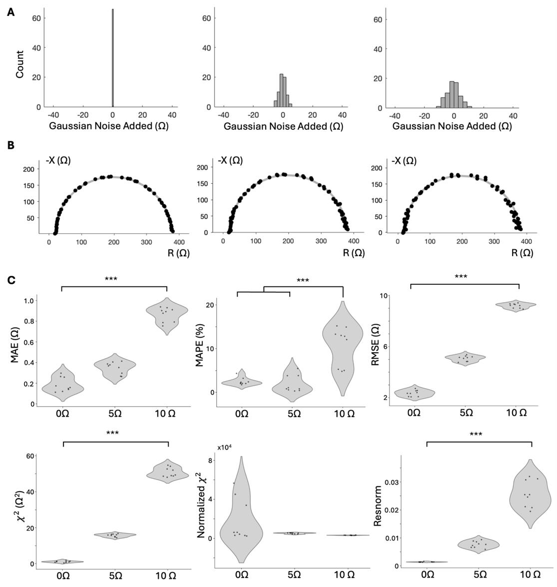
Figure 12. Error comparison for measurements with Gaussian noise added. (A) Error added to RPE data from distributions N(0, 52), N(0, 102) (n = 3 samples and technical replicates). (B) Representative Nyquist plots illustrating the varying noise added. (C) Violin plots showing mean absolute error (MAE), mean absolute percent error (MAPE), root mean squared error (RMSE), χ2, normalized χ2, and resnorm metrics for original data and data with 5 Ω and 10 Ω s.d. Gaussian noise added. ANOVA and Tukey HSD statistical tests were used to determine significance. (*** Tukey HSD, p < 0.001, 1-way ANOVA, α < 0.05, p < 0.01). Individual Nyquist plots of the original data in Figure S4.
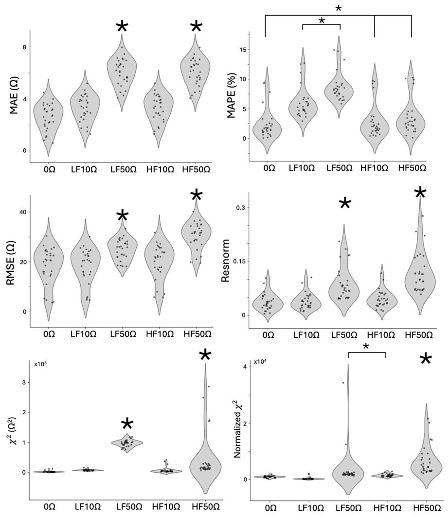
Figure 13. Error comparison for measurements with single-frequency error added on data from four 16HBE samples day 3–9. 10 Ω and 50 Ω error added to the resistance and reactance of 2 Hz (low frequency, LF) and 50 kHz (high frequency, HF) 16HBE datapoints (n = 28). Violin plots showing mean absolute error (MAE), mean absolute percent error (MAPE), root mean squared error (RMSE), resnorm, χ2, and normalized χ2 metrics for original data and data with 5 Ω and 10 Ω s.d. Gaussian noise added. 1-way ANOVA and Tukey HSD statistical tests were used to determine significance. Tukey HSD, p < 0.001, ANOVA, α < 0.05, p < 0.0001). (Groups with large * are statistically different from groups without; a small * indicates statistical differences between two groups connected, e.g., MAPE * indicates that LF10Ω and LF50Ω are statistically different from the remaining groups. Individual Nyquist plots of the original data in Figure S3.
D. Protocol for data analysis
To run the nonlinear least squares fit on the raw impedance data to calculate the TER, TEC, and membrane ratio (α), the impedance data files need to be copied into a specific folder, and a lookup table must be made with the cross-sectional area of each sample. Once run, the fitting code writes a summary table that outputs the TER, TEC, α, and circuit fit values. Using the summary table and raw data, a MATLAB script is then used to calculate the mean absolute error for assessing the accuracy of the fit values.
1. Open the downloaded “extracellularEIS-main” folder from GitHub. Copy and paste the template lookup table in the “lookup table” folder titled “Template Lookup Table.xlsx” and rename the copy with your experiment name (e.g., “20240706Exp1 Lookup Table.xlsx”).
2. In the renamed lookup table, copy the name(s) of the raw data text file(s) (e.g., data1_freq.txt) you would like to fit into Column B, under “plateID.”
3. Type the cross-sectional area of the sample for each raw file in Column K under “measArea” (1.12 cm2 for Corning 3460 cell culture inserts).
4. Number the files in column A with integer values starting at 1.
5. Save and close the lookup table.
6. Copy all the raw impedance data files output by the NOVA software into the “raw data” folder in the “extracellularEIS-main” folder.
7. Open the “NOVA_batch_20240125.m” file in MATLAB and change the file name and path in line 51 to point to the desired lookup table (e.g., “20240706Exp1 Lookup Table.xlsx”).
8. In the MATLAB software, click the Editor menu in the top bar, and then the Run button to begin fitting. The software runs multiple fits in parallel and should show parallel processing in the lower left corner. A figure will pop up and update with the raw data Nyquist plots and the overlaid fit line as the fit code is running through each sweep.
9. When completed, a file with the format “lookupTableName_summary_table.csv” will be generated in the “FIT” folder. The parameters output into the CSV file are listed in Table 3.
Table 3. Fit values calculated by nonlinear least squares fitting, output in summary table CSV file
| Parameter | Unit | Description |
|---|---|---|
| RtArea | Ω·cm2 | (R1 + R2) × Area where Area is the cross-sectional area of the cell culture insert. |
| RblankArea | Ω·cm2 | Rsol × Area where Area is the cross-sectional area of the cell culture insert. |
| CtArea | μF/cm2 | Transepithelial capacitance, normalized to the cross-sectional area. |
| R1Area | Ω·cm2 | R1 × Area where Area is the cross-sectional area of the cell culture insert. |
| R2Area | Ω·cm2 | R2 × Area where Area is the cross-sectional area of the cell culture insert. |
| C1Area | μF/cm2 | C1/Area where Area is the cross-sectional area of the cell culture insert. |
| C2Area | μF/cm2 | C2/Area where Area is the cross-sectional area of the cell culture insert. |
| EVOMresistanceArea | Ω·cm2 | Resistance measured at 12.5 Hz, used for comparison with single-frequency measurements. |
| tauMEM | Unitless | Membrane ratio, α. |
| Exitflag | [-2, 4] | Exit flag indicating the condition under which the least squares algorithm ended. -2 = no feasible point found, and solver stopped at an infeasible point. -1 = function stopped the solver. 0 = number of iterations exceeds the max iterations set (default 400). 1 = function converged. 2 = change in the error function is less than the specified tolerance (default 1E-6). 3 = change in residual is less than the specified tolerance. 4 = relative magnitude of the search direction is smaller than the step tolerance (default 1E-6). |
10. The MAE can then be calculated using the “calcMAE.m” program from the “otherCode” folder in the downloaded GitHub folder. Open the program in MATLAB and change line 2 to reference the folder where the raw data is located (e.g., dataLocation = ‘/Users/myuser/rawData/’;).
11. Change line 5 to reference the location of the summary table with the fit values (e.g., SummaryTable = readtable(‘/Users/myuser/eisExtracellular/fit/20240706exp1_summary_table.csv’);).
12. Click the run button in the top toolbar. The code writes a file titled “errors.txt” with the filenames in the first column, MAE in the second, and resnorm in the third column, written to the same folder as the program.
Validation of protocol
We applied the method described to both RPE and 16HBE in order to provide examples of representative data from healthy cells. Figure 14 shows the resulting TER, TEC, and membrane ratio, α, on three samples of mature iPSC-RPE [4,24] and four samples of 16HBE (cultured to maturity, measured on day 7 [23]). The RPE cells have an average TER of 587 Ω·cm2, an average TEC of 3.8 μF/cm2, and an average α of 2.0. The measurements are repeatable, with TER 500–667 Ω·cm2 and TEC 3.65–4.10 μF/cm2. The 16HBE cells have an average TER of 983 Ω·cm2, an average TEC of 1.1 μF/cm2, and an average α of 20.0. The 16HBE measurements are also repeatable, with a narrower range for TER 955–1,034 Ω·cm2, and TEC 1.07–1.10 μF/cm2. These TER values are within the accepted threshold in literature for RPE [32,33] and 16HBE [23]; other metrics of TEC and
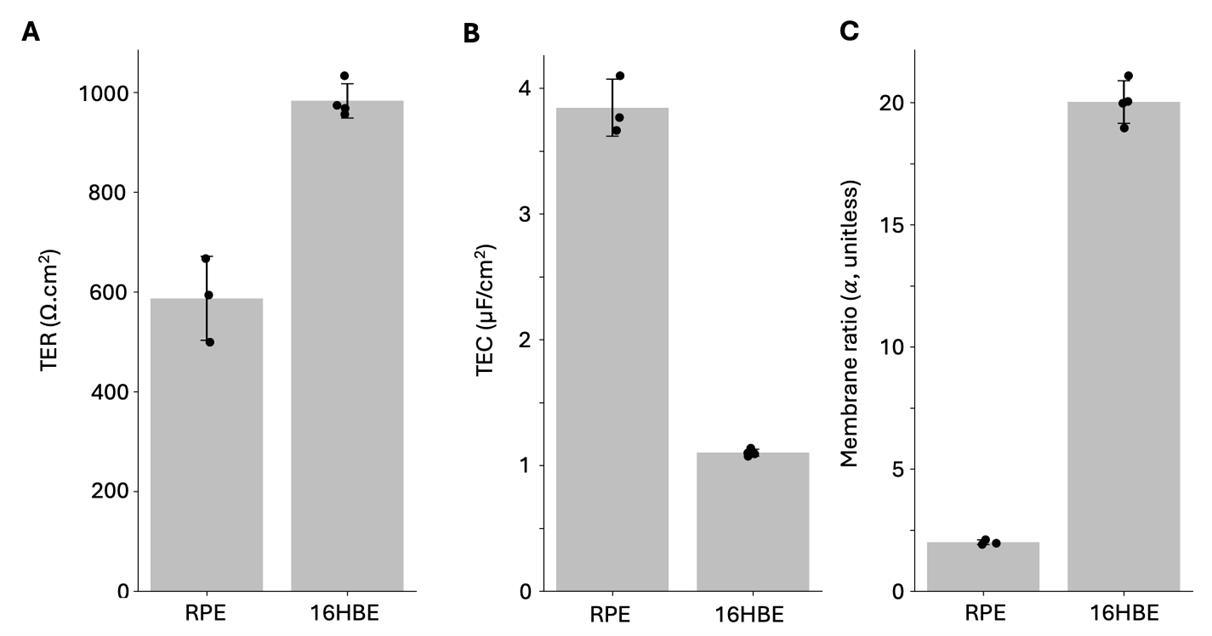
Figure 14. (A) TER, (B) TEC, and (C) membrane ratio measurements on mature RPE cells (n = 3) and 16HBE cells (n = 4, day 7) from frequency sweep 2 Hz–50 kHz, 4 μA fit to RCRC model in Figure 1D. Individual Nyquist plots are provided in Figures S3 and S4, and fit values TER, TEC, Rsol, R1, R2, C1, and C2 are in the summary tables provided in the GitHub repository. Error values are in Figures 12 and 13 (0 Ω groups). MAE was less than 6 Ω for all 16HBE samples (n = 4) and 1 Ω for all RPE samples (n = 3).
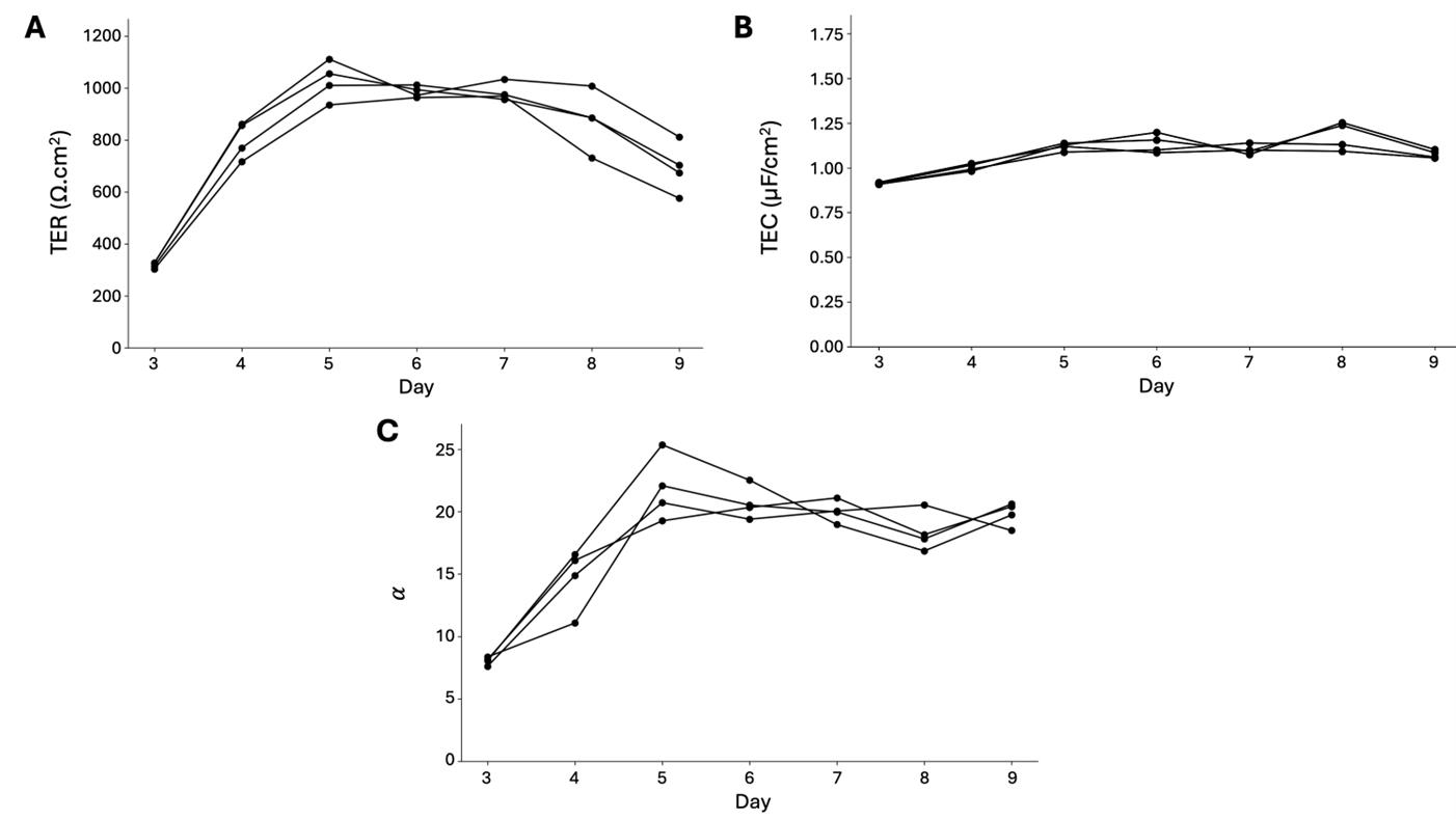
Figure 15. (A) TER, (B) TEC, and (C) membrane ratio αreported for 16HBE days 3–9 (n = 4) from frequency sweep 2 Hz–50 kHz, 5sines, 2 freq/dec., 4 μA fit to RCRC model in Figure 1D. Individual Nyquist plots are provided in Figure S3, and fit values TER, TEC, Rsol, R1, R2, C1, and C2 are in the summary tables provided in the GitHub repository. MAE was less than 10 for all samples.
We have also used this technique to monitor EIS of bronchiolar epithelial cells, for example, in a study of days 3–9 after seeding, reporting TER, TEC, and membrane ratios each day (Figure 15). The TER trend shows that the bronchiolar cells reach their highest TER by day 5 and maintain stable until day 8, while the TEC is stable around 1 μF/cm2 at days 5–9. The membrane ratio, similar to TEC, rises from day 3 to 5, before stabilizing around 20 through day 9.
All data and code have been deposited to GitHub: https://github.com/chien0507/extracellularEIS.git (access date, 03/13/2025).
General notes and troubleshooting
General notes
1. Is there a way to estimate TER and TEC directly from the Nyquist plot?
Visually, the transepithelial resistance (TER) can be determined on the Nyquist plot as the difference between the two intersections with the real or resistance axis [848 - 37 = 811 Ω normalized to the cross-sectional area 1.12 cm2 (908 Ω·cm2) as shown in Figure 11A or 626 Ω·cm2 as shown in Figure 11B]. TEC for this RCRC model is more difficult to determine directly from the Nyquist plot, but each local maximum on the Nyquist plot can be used to determine the individual capacitances contributing if R1 and R2 are known, because ωRC = 1 at these points, as labeled in Figure 2. For more information on interpreting Nyquist plots and understanding the foundations of electrochemical impedance spectroscopy, we recommend the following sources: Gerhardt [21] and Gerasimenko [34].
2. What is the expected exit flag for good fits?
Typically, the exit flag for good fits is 3, indicating the change in the residual is less than the specified tolerance, and the measurements of solution alone or a blank transwell are 1, indicating that the function converged.
3. How does temperature affect TER?
TER varies depending on the cell environment. Blume et al. discussed the variability in TER due to temperature [35]. Atmospheric changes due to changes in environmental conditions or solutions can also cause significant effects on the cells. The temperature dependence has only been reported on TER, but to try to measure as closely to physiologic conditions as possible in Ussing chamber studies, cells are typically maintained at physiological temperatures. However, one-time measurement of TER is commonly measured in the cell culture hood at room temperature because these conditions are easier to replicate, and relative changes in TER can still be reported and have biological significance.
4. How do media changes affect TER?
We do not recommend changing media prior to measurement, as we have observed cells change impedance rapidly following a media change. Instead, change the media after the measurement or several hours before the experiment to allow the cells to stabilize.
5. How frequently can you perform EIS in the EndOhm?
Silver chloride electrodes, like those used in the EndOhm, are used for rapid signal transmission but are meant for short-term measurements, as silver is a known toxin for cells. The chloride layer, preventing such toxicity, can easily be scraped off or nicked, having dose-dependent toxic effects [34,36,37]. However, exposure with smaller silver chloride electrodes has been used in alternative setups [38].
6. Should the electrodes look shiny or have shiny spots?
No, the electrodes should be coated in chloride ions, giving them a dull grey color (see Figure 16). Stripping of the chloride layer, exposing the shiny silver layer underneath, can result in unexpected toxicity, and results in fewer chloride ions readily available to move in solution, making the signal sent across the cells unreliable.
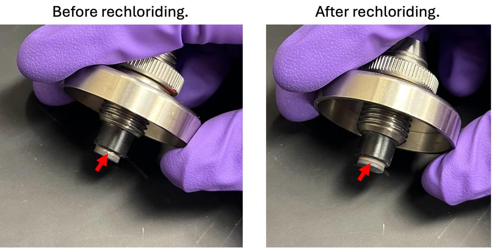
Figure 16. EndOhm cap in need of rechloriding (left) and showing a shiny finish on the apical working electrode, and showing the dull finish after rechloriding (right) due to the chloride layer
If the silver is showing, follow the instructions to rechloride [39]. Briefly, fill the EndOhm with sodium hypochlorite solution. Let the electrodes soak for 10 min. Electrode should appear darker in color. Rinse with deionized water.
7. Are there known effects of these electrical measurements on cell behavior?
Electrophysiology measurements for functional analyses can be non-invasive; cells measured on whole cell culture inserts and only extracellularly (without penetrating them) can be returned to culture for later use and assessed multiple times. Generally, to minimize stimulation, magnitudes are kept below tens of microamps and several millivolts to prevent changes in activation of ion channels, cell shape, migration, and proliferation, although the exact values depend on the electrode type, culture media, and type of cells [34]. However, it is important to note that sending larger voltages or currents may influence the cell response, used to stimulate cells in conductive, inductive, or capacitive coupled systems [40]. For example, in bone marrow mesenchymal stromal cells, it has been shown that the membrane voltage can be manipulated to control proliferation using a direct current signal of hundreds of millivolts [41].
Troubleshooting
Problem 1: Impedance sweeps show more noise than previously measured (see Figure 10A).
Possible cause: Electrodes are not fully submerged, or bubbles are present on the electrode surface.
Solution: If bubbles appear, lift and reset the cap and cell culture insert, or pipette media toward the bubbles to dislodge and pop them from the bottom of the EndOhm. If electrodes are not fully submerged, add more media to the chamber.
Problem 2: Nyquist plot shows a nearly vertical line (see Figure 10B).
Possible cause: The cable is not connected, or the device is not running on the correct channel.
Solution: Check if all cables are connected as described, ensuring the plug into the EndOhm chamber is dry, and rerun selecting the correct channel.
Supplementary information
The following supporting information can be downloaded here:
1. Figure S1. Additional reference images for adapter fabrication.
2. Figure S2. Rsol, R1, R2, C1, and C2 values for 4 test circuits, 6 technical replicates, 6 fits, showing the true values (top), bar chart of the raw values (middle), and error values (bottom).
3. Figure S3. Nyquist plots (Y-axis negative reactance, x-axis resistance in Ω) for all four 16HBE samples from day three to day nine, with overlaid fit line.
4. Figure S4. Nyquist plots (Y-axis negative reactance, x-axis resistance in Ω) for all six RPE samples, showing fit line and raw data.
Acknowledgments
Conceptualization, A.J.C., C.L., A.L.W., C.H.; Investigation, A.J.C., C.L., H.K., A.V.C.; Writing—Original Draft, A.J.C.; Writing—Review & Editing, A.J.C., C.F., H.K., R.G., N.M.; Funding Acquisition, A.J.C., C.F.; Supervision, C.F., N.M., K.B. Prior work in Lewallen et al. [1] from which the fitting code is derived.
Thanks to the research group of Dr. Kapil Bharti at the National Eye Institute within the National Institutes for Health for culturing and providing mature iPSC-RPE cells and media. This material is based upon work supported by the National Science Foundation Graduate Research Fellowship under Grant No. (DGE-2039655). Any opinion, findings, and conclusions or recommendations expressed in this material are those of the authors(s) and do not necessarily reflect the views of the National Science Foundation. CRF acknowledges the NIH BRAIN Initiative Grant (NEI and NIMH 1-U01-MH106027-01), NIH R01NS102727, NIH Single Cell Grant 1 R01 EY023173, NIH R01DA029639, and NIH RF1AG079269, support from Georgia Tech through the Institute for Bioengineering and Biosciences, Invention Studio, and the George W. Woodruff School of Mechanical Engineering. OpenAI’s GPT-4 was used in the preparation of this document to generate initial drafts of the abstract and introduction sections that have since been further refined.
Competing interests
This research was partially supported under a Sponsored Research Agreement between the Georgia Tech Research Corporation and World Precision Instruments. C.R. Forest, C. Lewallen, and K. Bharti, as well as A. Maminishkis are co-inventors on a patent pending related to this protocol, entitled “Apparatus and method for Extracellular Impedance Spectroscopy of epithelia”, filed Jan 15, 2024, GTRC 9153, utility application 18/412,842, and PCT filed. The patent is exclusively licensed by Georgia Tech Research Corporation and National Institute of Health to World Precision Instruments, Sarasota FL.
References
- Lewallen, C. F., Chien, A., Maminishkis, A., Hirday, R., Reichert, D., Sharma, R., Wan, Q., Bharti, K. and Forest, C. R. (2023). A biologically validated mathematical model for decoding epithelial apical, basolateral, and paracellular electrical properties. Am J Physiol Cell Physiol. 325(6): C1470–C1484. https://doi.org/10.1152/ajpcell.00200.2023
- Linz, G., Djeljadini, S., Steinbeck, L., Köse, G., Kiessling, F. and Wessling, M. (2020). Cell barrier characterization in transwell inserts by electrical impedance spectroscopy. Biosens Bioelectron. 165: 112345. https://doi.org/10.1016/j.bios.2020.112345
- Hassan, Q., Ahmadi, S. and Kerman, K. (2020). Recent Advances in Monitoring Cell Behavior Using Cell-Based Impedance Spectroscopy. Micromachines.11(6): 590. https://doi.org/10.3390/mi11060590
- Miyagishima, K. J., Wan, Q., Corneo, B., Sharma, R., Lotfi, M. R., Boles, N. C., Hua, F., Maminishkis, A., Zhang, C., Blenkinsop, T., et al. (2016). In Pursuit of Authenticity: Induced Pluripotent Stem Cell-Derived Retinal Pigment Epithelium for Clinical Applications. Stem Cells Transl Med. 5(11): 1562–1574. https://doi.org/10.5966/sctm.2016-0037
- Blazer-Yost, B. L. (2022). Following Ussing’s legacy: from amphibian models to mammalian kidney and brain. Am J Physiol Cell Physiol. 323(4): C1061–C1069. https://doi.org/10.1152/ajpcell.00303.2022
- Cui, G., Cottrill, K. A. and McCarty, N. A. (2021). Electrophysiological Approaches for the Study of Ion Channel Function. Methods Mol Biol. 2302: 49–67. https://doi.org/10.1007/978-1-0716-1394-8_4
- Srinivasan, B., Kolli, A. R., Esch, M. B., Abaci, H. E., Shuler, M. L. and Hickman, J. J. (2015). TEER Measurement Techniques for In Vitro Barrier Model Systems. SLAS Technol. 20(2): 107–126. https://doi.org/10.1177/2211068214561025
- Yeste, J., Illa, X., Gutiérrez, C., Solé, M., Guimerà, A. and Villa, R. (2016). Geometric correction factor for transepithelial electrical resistance measurements in transwell and microfluidic cell cultures. J Phys D: Appl Phys. 49(37): 375401. https://doi.org/10.1088/0022-3727/49/37/375401
- Lewallen, C. F., Wan, Q., Maminishkis, A., Stoy, W., Kolb, I., Hotaling, N., Bharti, K. and Forest, C. R. (2019). High-yield, automated intracellular electrophysiology in retinal pigment epithelia. J Neurosci Methods. 328: 108442. https://doi.org/10.1016/j.jneumeth.2019.108442
- Cottrill, K. A., Peterson, R. J., Lewallen, C. F., Koval, M., Bridges, R. J. and McCarty, N. A. (2021). Sphingomyelinase decreases transepithelial anion secretion in airway epithelial cells in part by inhibiting CFTR‐mediated apical conductance. Physiol Rep. 9(15): e14928. https://doi.org/10.14814/phy2.14928
- Tervonen, A., Ihalainen, T. O., Nymark, S. and Hyttinen, J. (2019). Structural dynamics of tight junctions modulate the properties of the epithelial barrier. PLoS One. 14(4): e0214876. https://doi.org/10.1371/JOURNAL.PONE.0214876
- Felix, K., Tobias, S., Jan, H., Nicolas, S. and Michael, M. (2021). Measurements of transepithelial electrical resistance (TEER) are affected by junctional length in immature epithelial monolayers. Histochem Cell Biol. 156(6): 609–616. https://doi.org/10.1007/S00418-021-02026-4/FIGURES/4
- Claude, P. (1978). Morphological factors influencing transepithelial permeability: A model for the resistance of the Zonula Occludens. J Membr Biol. 39(2–3): 219–232. https://doi.org/10.1007/BF01870332/METRICS
- Kreindler, J. L., Jackson, A. D., Kemp, P. A., Bridges, R. J. and Danahay, H. (2005). Inhibition of chloride secretion in human bronchial epithelial cells by cigarette smoke extract. Am J Physio. - Lung Cell Mol Physiol. 288(5 32–5): 894–902. https://doi.org/10.1152/AJPLUNG.00376.2004
- Schimetz, J., Shah, P., Keese, C., Dehnert, C., Detweiler, M., Michael, S., Toniatti-Yanulavich, C., Xu, X. and Padilha, E. C. (2024). Automated measurement of transepithelial electrical resistance (TEER) in 96-well transwells using ECIS TEER96: Single and multiple time point assessments. SLAS Technol. 29(1): 100116. https://doi.org/10.1016/J.SLAST.2023.10.008
- Lim, J. J. and Fischbarg, J. (1981). Electrical properties of rabbit corneal endothelium as determined from impedance measurements. Biophys J. 36(3): 677–695. https://doi.org/10.1016/S0006-3495(81)84758-3
- Clausen, C., Lewis, S. and Diamond, J.(1979). Impedance analysis of a tight epithelium using a distributed resistance model. Biophys J. 26(2): 291–317. https://doi.org/10.1016/s0006-3495(79)85250-9
- Müller, S., Ebert, F., Bornhorst, J., Galla, H. J., Francesconi, K. and Schwerdtle, T. (2018). Arsenic-containing hydrocarbons disrupt a model in vitro blood-cerebrospinal fluid barrier. J Trace Elem Med Biol. 49: 171–177. https://doi.org/10.1016/j.jtemb.2018.01.020
- Onnela, N., Savolainen, V., Juuti-Uusitalo, K., Vaajasaari, H., Skottman, H. and Hyttinen, J. (2012). Electric impedance of human embryonic stem cell-derived retinal pigment epithelium. Med Biol Eng Comput. 50(2): 107–116. https://doi.org/10.1007/S11517-011-0850-Z/TABLES/2
- Schifferdecker, E. and Frömter, E.(1978). The AC impedance of necturus gallbladder epithelium. Eur J Physiol. 377(2): 125–133. https://doi.org/10.1007/bf00582842
- Gerhardt, R. A. (2024). Spectroscopy: Impedance spectroscopy and mobility spectra. Encycl Condens Matter Phys. 266–299. https://doi.org/10.1016/b978-0-323-90800-9.00021-4
- Chien, A., Lewallen, C., Cui, G., Cegla, A. V., Lull, E., Khor, H., McCarty, N. A. and Forest, C. (2025). BPS2025 - Rapid and accurate transepithelial resistance measurement of bronchiolar epithelium using impedance spectroscopy and RCRC model. Biophys J. 124(3): 296a–297a. https://doi.org/10.1016/j.bpj.2024.11.1658
- Vazquez Cegla, A. J., Jones, K. T., Cui, G., Cottrill, K. A., Koval, M. and McCarty, N. A. (2024). Effects of hyperglycemia on airway epithelial barrier function in WT and CF 16HBE cells. Sci Rep. 14(1): 1–12. https://doi.org/10.1038/s41598-024-76526-3
- Sharma, R., Bose, D., Montford, J., Ortolan, D. and Bharti, K. (2022). Triphasic developmentally guided protocol to generate retinal pigment epithelium from induced pluripotent stem cells. STAR Protoc. 3(3): 101582. https://doi.org/10.1016/j.xpro.2022.101582
- Miyagishima, K. J., Sharma, R., Nimmagadda, M., Clore-Gronenborn, K., Qureshy, Z., Ortolan, D., Bose, D., Farnoodian, M., Zhang, C., Fausey, A., et al. (2021). AMPK modulation ameliorates dominant disease phenotypes of CTRP5 variant in retinal degeneration. Commun Biol. 4(1): 1–16. https://doi.org/10.1038/s42003-021-02872-x
- Cystic Fibrosis Foundation. (n.d.). 16HBE14o-(WT CFTR) Cell Line Notes.
- Santoni, F., De Angelis, A., Moschitta, A., Carbone, P., Galeotti, M., Cinà, L., Giammanco, C. and Di Carlo, A.(2024). A guide to equivalent circuit fitting for impedance analysis and battery state estimation. J Energy Storage. 82: 110389. https://doi.org/10.1016/j.est.2023.110389
- Bello-Reuss, E. (1986). Cell membranes and paracellular resistances in isolated renal proximal tubules from rabbit and Ambystoma. J Physiol. 370(1): 25–38. https://doi.org/10.1113/jphysiol.1986.sp015920
- Kottra, G. and Frömter, E. (1984). Rapid determination of intraepithelial resistance barriers by alternating current spectroscopy. Pflugers Arch. 402(4): 421–432. https://doi.org/10.1007/bf00583943
- Kottra, G. and Frömter, E. (1993). Tight-junction tightness of Necturus gall bladder epithelium is not regulated by cAMP or intracellular Ca2+. Pflugers Arch. 425: 535–545. https://doi.org/10.1007/bf00374882
- Miller, S. S. and Steinberg, R. H.(1977). Passive ionic properties of frog retinal pigment epithelium. J Membr Biol. 36(1): 337–372. https://doi.org/10.1007/bf01868158
- Bharti, K., Ortolan, D. and Sharma, R. (2022). Methods to generate macular, central and peripheral retinal pigment epithelial cells (Patent No. US20240271089A1).
- Sharma, R., Khristov, V., Rising, A., Jha, B. S., Dejene, R., Hotaling, N., Li, Y., Stoddard, J., Stankewicz, C., Wan, Q., et al. (2019). Clinical-grade stem cell–derived retinal pigment epithelium patch rescues retinal degeneration in rodents and pigs. Sci Transl Med. 11(475): eaat5580. https://doi.org/10.1126/scitranslmed.aat5580
- Gerasimenko, T., Nikulin, S., Zakharova, G., Poloznikov, A., Petrov, V., Baranova, A. and Tonevitsky, A.(2020). Impedance Spectroscopy as a Tool for Monitoring Performance in 3D Models of Epithelial Tissues. Front Bioeng Biotechnol. 7: e00474. https://doi.org/10.3389/fbioe.2019.00474
- Blume, L. F., Denker, M., Gieseler, F. and Kunze, T. (2010). Temperature corrected transepithelial electrical resistance (TEER) measurement to quantify rapid changes in paracellular permeability. Pharmazie. 65(1): 19–24. https://doi.org/10.1691/PH.2010.9665
- Grimnes, S. and Martinsen, Ø. G. (2015). Electrodes. Bioimpedance Bioelectr Basics. 179–254. https://doi.org/10.1016/B978-0-12-411470-8.00007-6
- Waleed Shinwari, M., Zhitomirsky, D., Deen, I. A., Selvaganapathy, P. R., Jamal Deen, M. and Landheer, D. (2010). Microfabricated reference electrodes and their biosensing applications. Sensors (Basel). 10(3). 1679–1715. https://doi.org/10.3390/S100301679
- Douville, N. J., Tung, Y. C., Li, R., Wang, J. D., El-Sayed, M. E. H. and Takayama, S. (2010). Fabrication of two-layered channel system with embedded electrodes to measure resistance across epithelial and endothelial barriers. Anal Chem. 82(6): 2505–2511. https://doi.org/10.1021/AC9029345
- World Precision Instruments. (2022). EndOhm Tissue resistance measurement chambers for tissue culture cups. Retrieved from https://www.wpiinc.com/
- Meneses, J., Fernandes, S., Alves, N., Pascoal-Faria, P. and Cavaleiro Miranda, P. (2022). How to correctly estimate the electric field in capacitively coupled systems for tissue engineering: a comparative study. Sci Rep. 12. https://doi.org/10.1038/s41598-022-14834-2
- Bhavsar, M. B., Leppik, L., Costa Oliveira, K. M. and Barker, J. H. (2020). Role of Bioelectricity During Cell Proliferation in Different Cell Types. Front Bioeng Biotechnol. 8: e00603. https://doi.org/10.3389/fbioe.2020.00603
Article Information
Publication history
Received: Mar 13, 2025
Accepted: May 9, 2025
Available online: May 30, 2025
Published: Jun 20, 2025
Copyright
© 2025 The Author(s); This is an open access article under the CC BY-NC license (https://creativecommons.org/licenses/by-nc/4.0/).
How to cite
Chien, A. J., Lewallen, C. F., Khor, H., Cegla, A. V., Guo, R., Watson, A. L., Hatcher, C., McCarty, N. A., Bharti, K. and Forest, C. R. (2025). Method for Extracellular Electrochemical Impedance Spectroscopy on Epithelial Cell Monolayers. Bio-protocol 15(12): e5341. DOI: 10.21769/BioProtoc.5341.
Category
Bioinformatics and Computational Biology
Biophysics > Electrophysiology > Electrochemical Impedance Spectroscopy
Cell Biology > Cell-based analysis > Electrophysiological technique
Do you have any questions about this protocol?
Post your question to gather feedback from the community. We will also invite the authors of this article to respond.