Development of a Novel Automated Workflow in Fiji ImageJ for Batch Analysis of Confocal Imaging Data to Quantify Protein Colocalization Using Manders Coefficient

Materials and reagents

Biological materials

1. HEK293 cells (American Type Culture Collection, CRL-1573)

2. pcDNA3.1(+)-WT-OATP1B1: pcDNA3.1 (+) vector-based mammalian expression plasmid vector with the open reading frame of wild-type (WT) OATP1B1 was subcloned at GenScript Biotech (Piscataway, NJ) and verified by sequencing, as described in our publication [9]

Reagents

1. Lipofectamine 2000 transfection reagent (Thermo Fisher Scientific, catalog number: 11668019)

2. Antibodies

Primary antibodies: Rabbit FLAG polyclonal antibody (Sigma-Aldrich, catalog number: F7425) and mouse monoclonal Na/K-ATPase antibody (Santa Cruz, catalog number: sc-21712)

Secondary antibodies: Alexa Fluor 594 goat anti-rabbit IgG (Thermo Fisher Scientific, catalog number: A-11012) and Alexa Fluor^® 488 goat anti-mouse IgG antibody (Thermo Fisher Scientific, catalog number: A-11001)

3. 4’,6-diamidino-2-phenylindole, dihydrochloride (DAPI) (Thermo Fisher Scientific, catalog number: D1306)

Equipment

1. Fluoview microscope (Olympus, model: FV10i-LIV Confocal Imaging System with Live-Cell)

2. Computer system (Windows 10 Enterprise, Processor: 12th Gen Intel^® Core^TM i5-12500, 3.00 GHz, RAM: 16.0 GB)Note: Any computer system capable of running Fiji ImageJ on supported platforms is acceptable.

Software and datasets

1. Fiji ImageJ (1.54f, 09/15/2024) [6], open source (https://imagej.net/Fiji/Downloads)

2. BIOP-JACoP (v2.1.1, 08/20/2010) installed to Fiji ImageJ:

Download JACoP from https://github.com/fabricecordelieres/IJ-Plugin_JACoP/releases/download/v2.1.4/JACoP_.jar. Launch Fiji, Help → Update → manage update sites. In the search box, type in PTBIOP → Apply and close → Apply changes → Close.

3. Python (v3.12.6, 09/06/2024), open source (https://www.python.org/downloads/)

4. GraphPad Prism (10.4.1, 12/05/2024), requires subscription (RRID:SCR_002798, https://www.graphpad.com)

4. All code and executable Windows applications have been deposited to GitHub and are publicly available: https://github.com/weiyue99/Yue-Colocalization (10/4/2024).

Procedure

The current protocol provides a detailed step-by-step procedure for conducting batch analysis to determine the Manders coefficient for colocalization quantification using confocal z-stack datasets from immunofluorescent staining. A detailed protocol for immunofluorescent staining and confocal imaging has been described in our previous publications [8,9]. In brief, HEK293 cells were transiently transfected with pcDNA3.1(+)-WT-OATP1B1 using Lipofectamine following the manufacturer’s instructions. Forty-eight hours after transfection, immunofluorescent staining was conducted using rabbit anti-FLAG (1:100 dilution) and mouse anti-Na/K-ATPase (1:50 dilution) antibodies [8,9] and detected by Alexa Fluor 594 and Alexa Fluor 488 conjugated goat anti-rabbit and goat-anti-mouse secondary antibodies, respectively. Nuclei were counter-stained by DAPI.

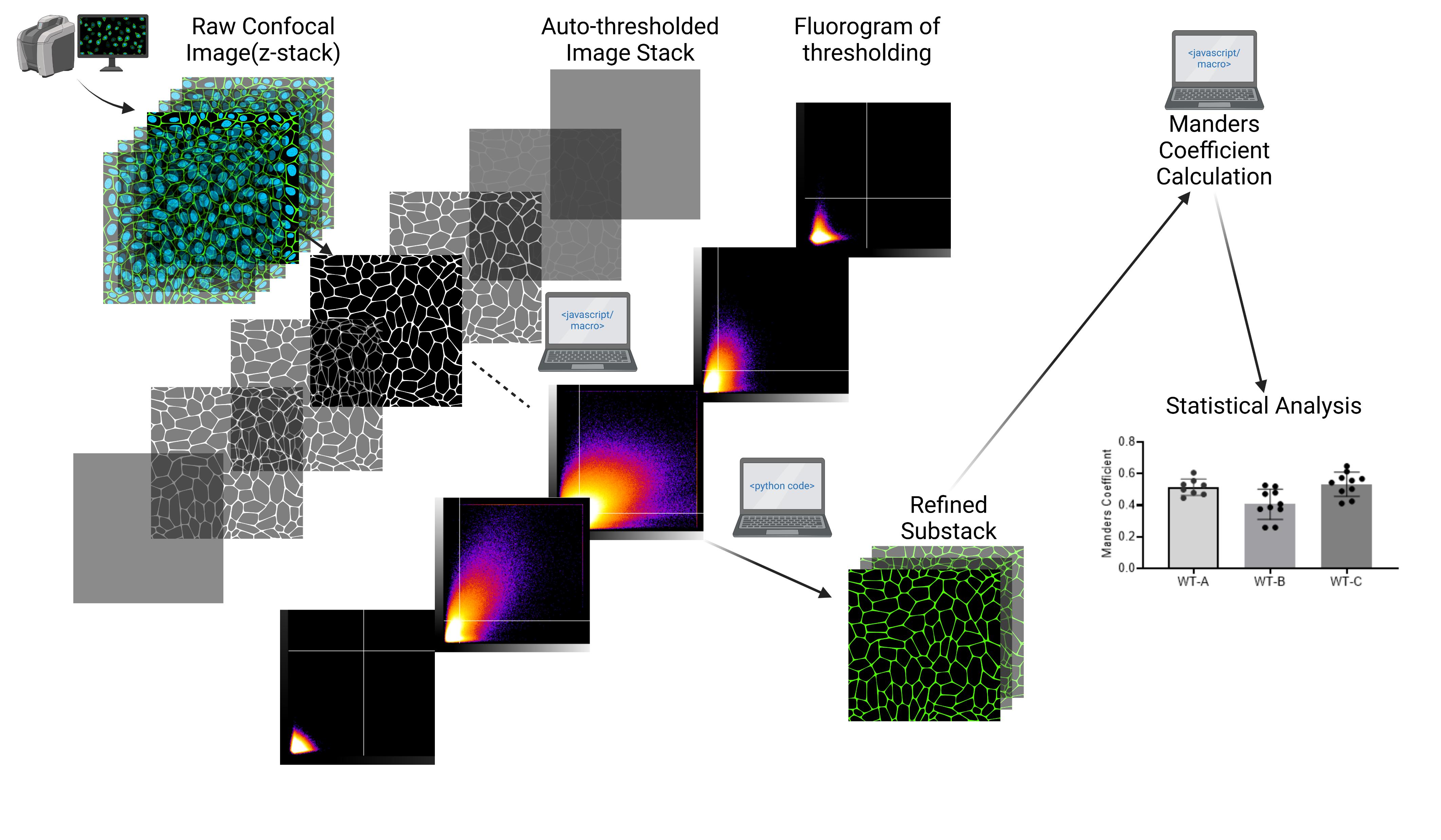
Confocal microscopy was conducted using an FV10i-LIV confocal microscope. Imaging was performed with excitation wavelengths of 405 nm (DAPI), 473 nm (Alexa Fluor 488), and 559 nm (Alexa Fluor 594). High-resolution images were captured at a matrix size of 1,024 × 1,024 pixels, with a pixel size of 0.207 μm and Z-slices spaced at 1 µm intervals, as described in our previous publication [9]. The current protocol uses WT-OATP1B1 data as an example (original Figure 8, WT in panels A–C from [9]). Signals of DAPI, Na/K-ATPase, and FLAG were designated to channels C1, C2, and C3, respectively. The extent of colocalization of FLAG-tagged OATP1B1 with Na/K-ATPase was determined by the Manders coefficient, which is the fraction of FLAG overlapping with Na/K-ATPase denoted as M2 in Image J output and used consistently throughout this manuscript. A brief overview of the current protocol is shown in Figure 1, followed by detailed step-by-step descriptions of each step.

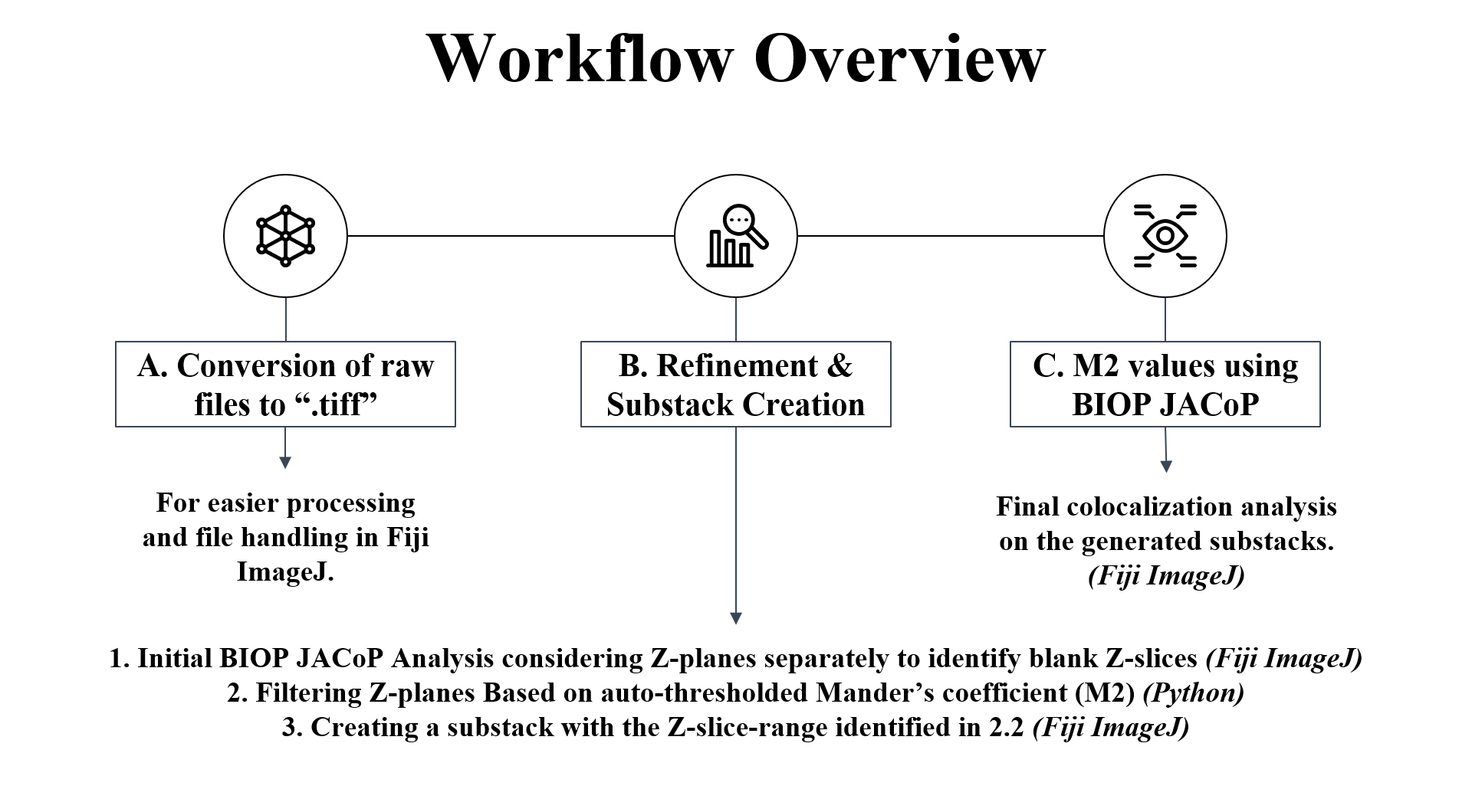
Figure 1. Workflow overview showing the key steps of the protocol. (A) Raw files are first converted to .tiff format in Fiji ImageJ. (B) Python code and Fiji ImageJ macro are utilized to refine and create substack images suitable for subsequent colocalization analysis in (C) to determine M2 values using the Manders coefficient method in Fiji ImageJ via the BIOP JACoP plugin.

A. Conversion of raw confocal files to .tiff files using Fiji ImageJ’s batch convert

The raw image files generated from confocal microscopy must be converted to .tiff format to enable compatibility with downstream analysis tools. This conversion is essential as the .tiff format is universally supported by image processing software, including Fiji ImageJ[6], and can be easily read and processed using JavaScript-based tools. The .tiff format ensures efficient handling of large image datasets while maintaining image fidelity and metadata.

Use the Batch Convert function in Fiji ImageJ for this process and organize the resulting .tiff images into a dedicated directory, preparing them for subsequent steps in the workflow.

1. Open Fiji ImageJ.

2. Go to Process → Batch →Convert… (Figure 2).

3. Select the folder containing the raw confocal image files in Input… and the folder where the .tiff files should be saved as Output… (Figure 3).

4. Interpolation: None.

5. Click Convert.

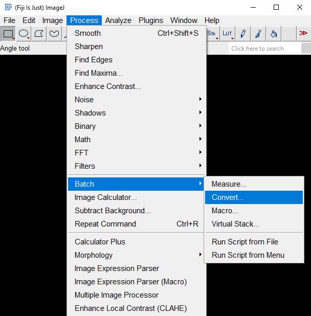
Figure 2. Screenshot of navigation through Fiji ImageJ to access the Batch Convert tool


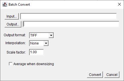
Figure 3. Screenshot of Batch Convert tool interface. Choose Input and Output file directory.

B. Image refinement and substack creation

Often, z-slices near the beginning and end of the z-stack have no fluorescent signal if these border z-slices are out of the range of thickness of the cells. In such z-slices, thresholded M2 values are reported as 0 or null (NaN) from the output of the BIOP JACoP. Follow the steps below to refine the Z-stack, creating a substack without slices containing 0 or null M2 values:

1. Initial BIOP JACoP batch Analysis in Fiji ImageJ to identify and locate blank Z-slices: Perform an initial auto-thresholding batch analysis using the BIOP JACoP plugin to determine Manders coefficients (M2), considering Z-planes separately. This analysis shows thresholded signals from each plane. The manual steps described below describe how to perform such analysis on one image file at a time. To process multiple images simultaneously, users should skip the Manual steps and directly proceed to the Batch analysis below.

Manual steps:

a. Open Fiji and load the raw image for analysis.

b. Go to Plugins → BIOP → Image Analysis → BIOP JACoP (Figure 4).

c. Choose the channel of interest for colocalization (Figure 5). For our dataset, assign Channel A as 2 (C2), which is the Na/K-ATPase signal, and assign Channel B as 3 (C3), which is the FLAG-OATP1B1 signal. The thresholding method is Otsu for both channels. Check to Consider Z-slices Separately, and select OK.

Note: Otsu is one of the auto-thresholding methods. The current protocol uses the commonly used Otsu [10] as an example. Refer to General note 1 for further optimizations.

d. Save the results as a .csv file in File → Save as.

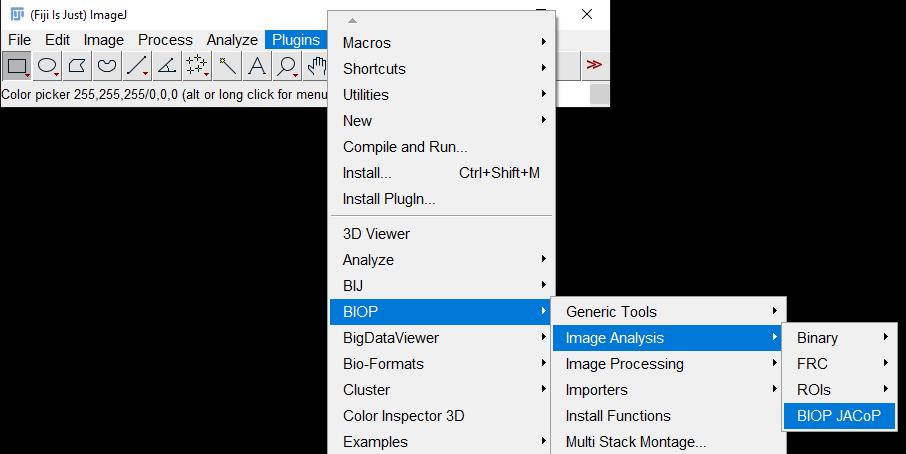
Figure 4. Screenshot of navigation through Fiji ImageJ to access the BIOP JACoP plugin


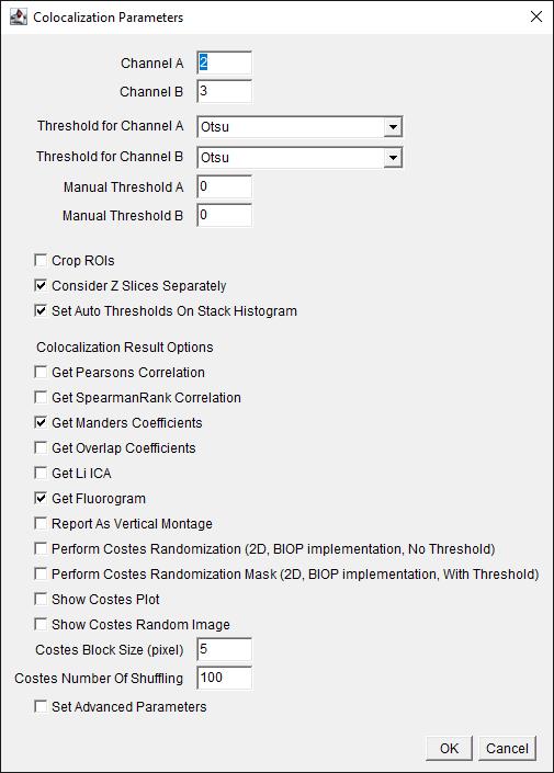
Figure 5. Screenshot of BIOP JACoP plugin’s Colocalization Parameters interface using Manders coefficient. Choose channels where the signal of interest is present. Choose the auto-thresholding (Otsu) method for each channel from the drop-down menu for Threshold for Channel. Check the boxes for options Consider Z Slices Separately, Set Auto Thresholds On Stack Histogram, Get Manders Coefficients, and Get Fluorogram.

Note: Our current protocol focuses on using the Manders Coefficient method [4] for colocalization determination. Using other methods listed on this interface for colocalization analysis is beyond the scope of our protocol. Users can refer to the BIOP-JACoP readme file https://imagej.net/plugins/coloc-2 and some original citations [11,12] for more information about other methods listed on this interface.

Batch analysis: Run the above manual steps process in batch mode using the following macro code in Fiji ImageJ. (Refer to General note 2 for how to run a macro code in Fiji ImageJ.) A screenshot is provided in Figure 6 after inputting the below macro code in Fiji ImageJ.

Note: This script analyzes all the image stacks in the root directory and generates the output in a single .csv file. This file contains thresholded Manders coefficient (M2) values for each Z-slice across all image stacks in the dataset. In the code, “//” denotes a comment in JavaScript.

setBatchMode(true);

//Locate file directory

inputDir = getDirectory("Select folder with .tiff files");

list = getFileList(inputDir);

//Make directory to save output files

resultsDir = inputDir +File.separator+"2_Results_zsclice_sep";

File.makeDirectory(resultsDir);

for (i = 0; i < list.length; i++)

{

          open(inputDir+list[i]);

 

          basename = list[i];

          basename_no_ext = File.getNameWithoutExtension(list[i]);

//Parameters for BIOP JACoP

    run("BIOP JACoP", "channel_a=2 channel_b=3 threshold_for_channel_a=Otsu threshold_for_channel_b=Otsu manual_threshold_a=0 manual_threshold_b=0 consider_z_slices_separately set_auto_thresholds_on_stack_histogram get_manders get_fluorogram costes_block_size=5 costes_number_of_shuffling=100");

    selectWindow(basename+" Report");

    saveAs("Tiff", resultsDir+File.separator+basename_no_ext+" Report.tif");

    close("*");

}

//Save results to output directory

saveAs("Results", resultsDir+File.separator+"AnalysisResults.csv");

selectWindow("Log");

saveAs("Text", resultsDir+File.separator+"AnalysisLog.txt");

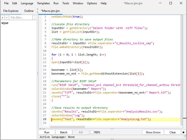
Figure 6. Screenshot of B.1 macro code in Fiji ImageJ

2. Find Z-planes with zero or null values using a Python script: Run the following Python script to identify ranges of positive M2 values, excluding null (NaN) or zero values. For each stack, it extracts the start and end Z-slice numbers corresponding to these positive ranges and generates a new .csv file that includes the image stack name and its Z-slice start and end numbers, facilitating precise substack creation for downstream analysis. A screenshot of Python code pasted in a text editor is provided in Figure 7. “#” denotes a comment in Python.

import pandas as pd

# Load the CSV with Manders coefficient results

file_path = 'path_to_csv/AnalysisResults.csv'

data = pd.read_csv(file_path)

# Filter for meaningful Z-slices with positive Thresholded M2 values

filtered_data = data[['Image A', 'Thresholded M2']]

filtered_data['Image Stack'] = filtered_data['Image A'].apply(lambda x: x.split(' ')[0])

positive_ranges = []

for image_stack, group in filtered_data.groupby('Image Stack'):

    group = group.reset_index(drop=True)

    positive_slices = group[group['Thresholded M2'] > 0].index.tolist()

    if positive_slices:

        first_z = positive_slices[0] + 1

        last_z = positive_slices[-1] + 1

        positive_ranges.append({

            'Image Stack': image_stack,

            'Positive Z-slices Start': first_z,

            'Positive Z-slices End': last_z

        })

# Save the filtered data

positive_ranges_df = pd.DataFrame(positive_ranges)

positive_ranges_df.to_csv('filtered_z_slices.csv', index=False)

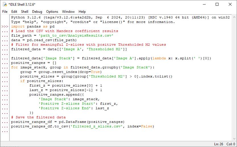
Figure 7. Screenshot of Python code in step B2 pasted in the Python editor as an example

Note: To run this script, the user must have Python v3.7 or above with the pandas library available in their computer system.

To minimize software dependency, we generated an executable Windows application and made it publicly available on GitHub (https://github.com/weiyue99/Yue-Colocalization) (Figure 8), allowing even those without Python experience to directly run this Python code (see also Troubleshooting). To do so:

a. Download the 3_filter_z_planes_app.exe from the above GitHub link. Right-click and Save link as → Save.

b. Double-click to run this application.

Note: You need admin privileges on your computer to allow this application for the first time.

c. A graphical user interface (GUI) dialog box will open (Figure 8). Select the .csv file generated in step B1 and click Open. The Python application will create a file positive_z_slices_ranges.csv in the same directory where the .exe application is present.

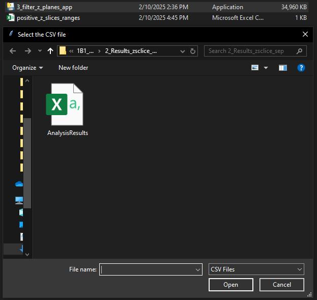
Figure 8. Screenshot of GUI dialog box that opens after executing the Python application (.exe) in Windows. Choose the AnalysisResults.csv file generated in Step B1 and click Open. The Python application will generate a positive_z_slices_ranges.csv file in the same directory where the .exe application is present.

3. Substack creation in Fiji ImageJ: The Make Substack... function in Fiji ImageJ is used to generate a substack from the raw .tiff files created in Section A. Each substack includes only two relevant channels and is limited to the Z-slice range identified in step 2. A screenshot is provided in Figure 9 after inputting the below macro code in Fiji ImageJ.

a. Run the following macro. (Refer to General note 2 for how to run a macro code in Fiji ImageJ.)

//Locate csv file with z-slice information

csvPath = File.openDialog("Select CSV file with Z-slice information");

inputDir = getDirectory("Select folder containing TIFF files");

//Make a directory to save output file

outputDir = inputDir + "subhyperstacks" + File.separator;

File.makeDirectory(outputDir);

//Read the csv file, and collect relevant columns

csvContent = File.openAsString(csvPath);

lines = split(csvContent, "\n");

imageNames = newArray();

startSlices = newArray();

endSlices = newArray();

for (i = 1; i < lines.length; i++) {

    tokens = split(lines[i], ",");

    //removes the channel name to match with file name, and collect start & end

    imageNames = Array.concat(imageNames, replace(tokens[0], "C2-", ""));

   startSlices = Array.concat(startSlices, parseInt(tokens[1]));

   endSlices = Array.concat(endSlices, parseInt(tokens[2]));

}

//Make substack

for (i = 0; i < imageNames.length; i++) {

    open(inputDir + imageNames[i]);

    run("Make Substack...", "channels=2-3 slices=" + startSlices[i] + "-" + endSlices[i]);

    //Save file

    saveAs("Tiff", outputDir + imageNames[i] + "_subhyperstack.tif");

    close();

}

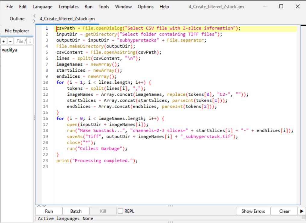
Figure 9. Screenshot of B3 macro code for substack creation in Fiji ImageJ

b. A dialog box will open. Select the filtered_z_slices.csv generated in step 2 and then select the folder containing the original .tiff files from Section A.

c. The macro will create new .tiff files containing two channels of interest with the filtered Z-planes.

C. Manders coefficient analysis on filtered substacks using BIOP JACoP

This step calculates the Manders coefficient (M2) to quantify the overlap between two signals of interest. In our case, this is Channel 2 (Na/K-ATPase) and Channel 3 (FLAG-OATP1B1) within the selected Z-slice range.

The “manual steps” below describe how to perform such analysis on one image file at a time. To process multiple images simultaneously, users should skip the Manual steps and directly proceed to the Batch analysis described below.

Manual steps:

1. Open Fiji and load the filtered substack for analysis.

2. Go to Plugins → BIOP → Image Analysis → BIOP JACoP (Figure 4).

3. Choose the channel of interest for colocalization. Here, it was C2: Na/K-ATPase and C3: FLAG. Thresholding method is Otsu, uncheckConsider Z slices Separately, and select OK (Figure 10).

4. Save the results as a .csv file in File → Save as.

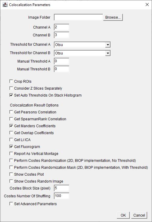
Figure 10. Screenshot of BIOP JACoP plugin’s Colocalization Parameters interface. Choose channels where the signal of interest is present. Choose the auto-thresholding method for each channel from the drop-down menu for Threshold for Channel. Check the boxes for options Set Auto Thresholds On Stack Histogram, Get Manders Coefficients, and Get Fluorogram.

Batch analysis:

To reduce hands-on time, run this process in batch mode using the following macro code. (Refer to General note 2 for how to run macro code in Fiji ImageJ.) A screenshot is provided in Figure 11 after inputting the below macro code in Fiji ImageJ.

setBatchMode(true);

//Locate file directory

inputDir = getDirectory("Select folder with .tiff files");

list = getFileList(inputDir);

//Make directory to save output files

resultsDir = inputDir +File.separator+"2_Results_zsclice_sep";

File.makeDirectory(resultsDir);

for (i = 0; i < list.length; i++)

{

     open(inputDir+list[i]);

     basename = list[i];

     basename_no_ext = File.getNameWithoutExtension(list[i]);

//Parameters for BIOP JACoP

    run("BIOP JACoP", "channel_a=1 channel_b=2 threshold_for_channel_a=Otsu threshold_for_channel_b=Otsu manual_threshold_a=0 manual_threshold_b=0 set_auto_thresholds_on_stack_histogram get_manders get_fluorogram costes_block_size=5 costes_number_of_shuffling=100");

    selectWindow(basename+" Report");

    saveAs("Tiff", resultsDir+File.separator+basename_no_ext+" Report.tif");

    close("*");

}

//Save results to output directory

saveAs("Results", resultsDir+File.separator+"AnalysisResults.csv");

selectWindow("Log");

saveAs("Text", resultsDir+File.separator+"AnalysisLog.txt");

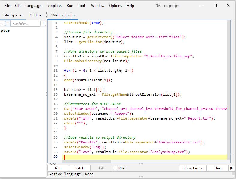
Figure 11. Screenshot of macro code of batch analysis from Section C in Fiji ImageJ

6. The results, including the final reports and analysis CSV, will be saved in a new folder named Results_Filtered within the input directory.

Data analysis

Manders coefficients depicting the colocalization of the protein of interest can be plotted using GraphPad Prism (RRID:SCR_002798).

Validation of protocol

This protocol has been used and validated in:

1. Tambe et al. [9]. Regulation of OATP1B1 Transport Function by Concurrent Phosphorylation and Lysine-Acetylation-A Novel Post-Translational Regulation Mechanism. Molecular Pharmacology (Figure 8, WT in panels A–C).

Three images from Figure 5B WT-OATP1B1 of the original publication are reused in Figure 12A of this manuscript. Manders coefficient values of WT-OATP1B1 (WT) in Figure 8A–C of the original publication are replotted here in Figure 12B. The reuse of previous data was approved by the journal.

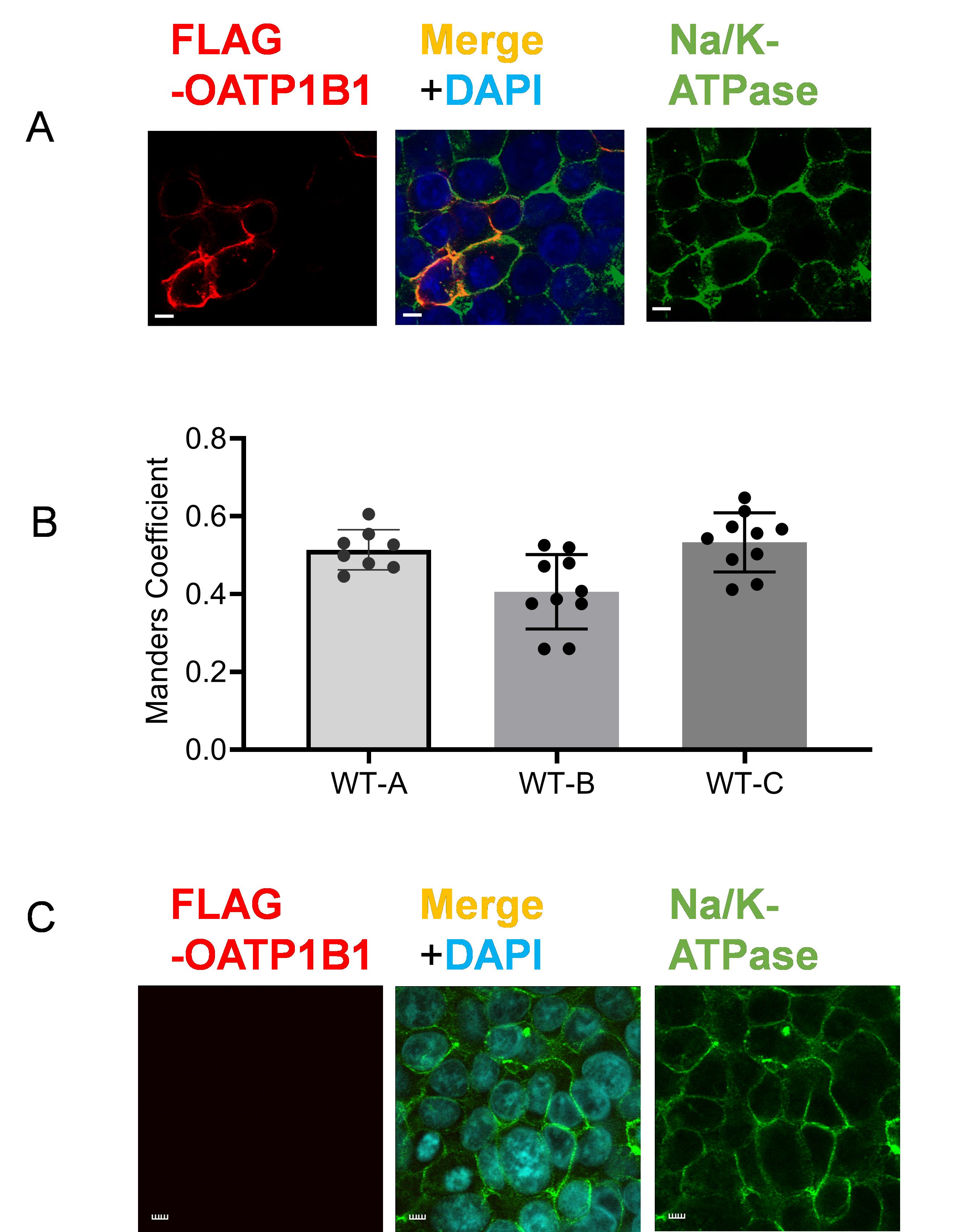
Figure 12. Quantitative colocalization analysis of FLAG-OATP1B1 and Na/K-ATPase in WT-OATP1B1. (A) Co-immunofluorescence staining of FLAG-tagged OATP1B1 (red) and Na/K-ATPase (green) in HEK293 cells 48 h post-transfection with WT-FLAG-OATP1B1. Nuclei were counterstained with DAPI. Representative images are shown. Scale bar, 10 µm. (B) Manders coefficient of colocalization of FLAG-OATP1B1 and Na/K-ATPase. Following the workflow described in this current protocol, confocal images in z-stack were utilized to determine Manders coefficients reflecting the fraction of FLAG-OATP1B1 colocalized with the Na/K-ATPase in WT-OATP1B1 transfected HEK293 cells in Figure 8A–C from [9]. WT-A, WT-B, and WT-C refer to the WT data in Figure 8A, B, and C, respectively, from the original publication [9]. Data represent mean ± SD. Each dot denotes data from replicates of confocal images. Figures are cited and modified from the following reference with permission: Tambe et al. (2025) Molecular Pharmacology, https://doi.org/10.1016/j.molpha.2024.100007 [9]. (C) FLAG and Na/K-ATPase (green) immunofluorescence staining in the negative control, non-transfected HEK293 cells. Nuclei were counterstained with DAPI.

General notes and troubleshooting

General notes

1. Ensuring consistent confocal image acquisition parameters across all samples in a dataset is crucial for reliable analysis. It is imperative to maintain uniform laser intensity and detector sensitivity settings across a dataset during image capture to facilitate accurate comparisons. Different specimens may respond better to specific thresholding methods; therefore, it is advisable to evaluate a sample image immediately after acquisition to determine the most suitable thresholding method.

To assess and select the optimal thresholding method in Fiji ImageJ, follow these steps:

a. Launch Fiji ImageJ and load one of your acquired raw images.

b. Navigate to Image → Adjust → Auto Threshold.

c. In the dialog box (Figure 13): Select the Try all option to apply multiple thresholding algorithms. Check the box labeled White objects on black background to ensure proper object-background distinction.

d. Click OK to generate a montage displaying the results of various thresholding methods applied to your image.

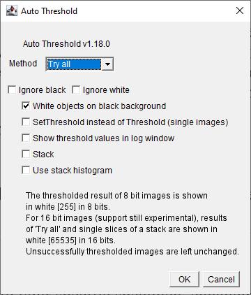
Figure 13. Screenshot of Auto Threshold interface. Select Try all option from the drop-down menu of Method. Check box for White objects on black background.

e. Review the montage to identify which thresholding method best suits your sample's characteristics. This procedure allows for the selection of the most effective thresholding technique tailored to your specific specimen, enhancing the accuracy of subsequent analyses.

2. Steps to run a macro in Fiji ImageJ:

a. Open Fiji.

b. Go to Plugins → New → Macro.

c. Copy and paste the macro code from the manuscript into the editor without modifying the indentations. For instance, in a for-loop, all nested commands must retain their original indentation; otherwise, the script may not be executed as intended.

d. Navigate to the menu bar and click on Run → Run.

Discussion

This protocol significantly reduced the hands-on time required to manually handle large quantities of image files. By automating the data processing, this approach also minimized the risk of human error associated with manual data handling. The protocol can complete the analysis in less than one hour of hands-on time, markedly enhancing efficiency and accuracy. In our current workflow, we utilized the Manders coefficient method and Otsu thresholding. This batch-processing workflow may be further developed and adapted based on this protocol to incorporate other colocalization methods in BIOP-JACoP plugin for determining colocalization. Thus, the protocol has the potential to have a broad impact in the field.

Troubleshooting

Problem 1: Out of memory.

Possible cause: Large image files and multiple analyses consume significant RAM, leading to slower performance or errors.

Solution: Optimize Fiji’s memory settings via Edit → Options → Memory & Threads... Allocate sufficient memory based on available computer system resources. For efficient processing, avoid running tasks on networked drives and transfer raw files to a local disk before initiating the workflow.

We successfully processed a 3.89 GB dataset (30 raw Z-stacks) using 12,970 MB of allocated memory in Fiji ImageJ, without encountering memory crashes.

Problem 2: Compatibility issues with plugins or code.

Possible cause: Outdated or incompatible versions of Fiji, BIOP-JACoP, or Python libraries can cause errors.

Solution: Ensure all software and plugins are updated to the specified versions listed in the protocol. For Python scripts, install the required libraries (e.g., pandas) using compatible Python versions (≥3.7). The standalone Python applet is available on GitHub: https://github.com/weiyue99/Yue-Colocalization

Acknowledgments

Specific contributions of each author: Conceptualization, V.A.; Investigation, V.A., V.T., and W.Y.; Writing—Original Draft, V.A. and W.Y.; Funding acquisition, W.Y. This research was supported by the National Institutes of Health NIH R01 GM146956-01 (W.Y.). The Olympus FV10i confocal microscope is supported by equipment grants from the NIH to Dr. Wei Yue (R01GM094268-06S1) and from the Presbyterian Health Foundation to Dr. Kelly Standifer. The current protocol was described and validated in a previous publication [9], and we acknowledge Mr. Ramon Kennedy, class of 2025 high school senior from the Oklahoma School of Science and Mathematics (OSSM) for testing the protocol. We acknowledge Dr. Pablo Ariel, Director of the Microscopy Services Laboratory at the University of North Carolina at Chapel Hill for the publicly shared materials from his “Colocalization Analysis Workshop” [13]. The initial code was created by ChatGPT [14]. The authors have refined, adapted, and validated these codes and are responsible for the correctness of the codes.

Competing interests

The authors declare no conflicts of interest.

References

1. Powell, J. T., Kayesh, R., Ballesteros-Perez, A., Alam, K., Niyonshuti, P., Soderblom, E. J., Ding, K., Xu, C. and Yue, W. (2023). Assessing Trans-Inhibition of OATP1B1 and OATP1B3 by Calcineurin and/or PPIase Inhibitors and Global Identification of OATP1B1/3-Associated Proteins. Pharmaceutics. 16(1): 63. https://doi.org/10.3390/pharmaceutics16010063
2. Jourdain, A. A., Koppen, M., Rodley, C. D., Maundrell, K., Gueguen, N., Reynier, P., Guaras, A. M., Enriquez, J. A., Anderson, P., Simarro, M., et al. (2015). A Mitochondria-Specific Isoform of FASTK Is Present In Mitochondrial RNA Granules and Regulates Gene Expression and Function. Cell Rep. 10(7): 1110–1121. https://doi.org/10.1016/j.celrep.2015.01.063
3. Aaron, J. S., Taylor, A. B. and Chew, T. L. (2018). Image co-localization – co-occurrence versus correlation. J Cell Sci. 131(3): e211847. https://doi.org/10.1242/jcs.211847
4. Manders, E. M. M., Verbeek, F. J. and Aten, J. A. (1993). Measurement of co‐localization of objects in dual‐colour confocal images. J Microsc. 169(3): 375–382. https://doi.org/10.1111/j.1365-2818.1993.tb03313.x
5. Liang, W., Sagar, S., Ravindran, R., Najor, R. H., Quiles, J. M., Chi, L., Diao, R. Y., Woodall, B. P., Leon, L. J., Zumaya, E., et al. (2023). Mitochondria are secreted in extracellular vesicles when lysosomal function is impaired. Nat Commun. 14(1): 5031. https://doi.org/10.1038/s41467-023-40680-5
6. Schindelin, J., Arganda-Carreras, I., Frise, E., Kaynig, V., Longair, M., Pietzsch, T., Preibisch, S., Rueden, C., Saalfeld, S., Schmid, B., et al. (2012). Fiji: an open-source platform for biological-image analysis. Nat Methods. 9(7): 676–682. https://doi.org/10.1038/nmeth.2019
7. Alam, K., Crowe, A., Wang, X., Zhang, P., Ding, K., Li, L. and Yue, W. (2018). Regulation of Organic Anion Transporting Polypeptides (OATP) 1B1- and OATP1B3-Mediated Transport: An Updated Review in the Context of OATP-Mediated Drug-Drug Interactions. Int J Mol Sci. 19(3): 855. https://doi.org/10.3390/ijms19030855
8. Crowe, A., Zheng, W., Miller, J., Pahwa, S., Alam, K., Fung, K. M., Rubin, E., Yin, F., Ding, K., Yue, W., et al. (2019). Characterization of Plasma Membrane Localization and Phosphorylation Status of Organic Anion Transporting Polypeptide (OATP) 1B1 c.521 T>C Nonsynonymous Single-Nucleotide Polymorphism. Pharm Res. 36(7): 101. https://doi.org/10.1007/s11095-019-2634-3
9. Tambe, V., Soderblom, E. J., Kayesh, R., Aditya, V., Xu, C. and Yue, W. (2025). Regulation of organic anion transporting polypeptide 1B1 transport function by concurrent phosphorylation and lysine-acetylation: A novel posttranslational regulation mechanism. Mol Pharmacol. 107(2): 100007. https://doi.org/10.1016/j.molpha.2024.100007
10. Otsu, N. (1979). A Threshold Selection Method from Gray-Level Histograms. IEEE Trans Syst Man Cybern. 9(1): 62–66. https://doi.org/10.1109/tsmc.1979.4310076
11. Costes, S. V., Daelemans, D., Cho, E. H., Dobbin, Z., Pavlakis, G. and Lockett, S. (2004). Automatic and Quantitative Measurement of Protein-Protein Colocalization in Live Cells. Biophys J. 86(6): 3993–4003. https://doi.org/10.1529/biophysj.103.038422
12. Li, Q., Lau, A., Morris, T. J., Guo, L., Fordyce, C. B. and Stanley, E. F. (2004). A Syntaxin 1, Gα_o, and N-Type Calcium Channel Complex at a Presynaptic Nerve Terminal: Analysis by Quantitative Immunocolocalization. J Neurosci. 24(16): 4070–4081. https://doi.org/10.1523/jneurosci.0346-04.2004
13. Ariel, P. (2024). Colocalization analysis workshop. (Accessed on 3.4.2025 https://cdr.lib.unc.edu/concern/multimeds/3j333c851)
14. OpenAI. (2024). ChatGPT (December 28 version) [Large language model]. Retrieved from https://openai.com/chatgpt