- Protocols

- Articles and Issues
- For Authors
- About
- Become a Reviewer

Dual-Modal Fast Photoacoustic/Ultrasound Localization Imaging with Sparsity-Constrained Optimization

(*contributed equally to this work) Published: Vol 15, Iss 6, Mar 20, 2025 DOI: 10.21769/BioProtoc.5247 Views: 3483
Reviewed by: Shun Yu Jasemine YangAnonymous reviewer(s)
Original research article
The authors used this protocol in:

Apr 2023
Advertisement


Protocol Collections
Comprehensive collections of detailed, peer-reviewed protocols focusing on specific topics


Abstract
Dual-modal imaging, combining photoacoustic (PA) and ultrasound localization (UL) with microbubbles, holds substantial promise across biomedical fields such as oncology, neuroscience, nephrology, and immunology. The combination of PA and UL imaging faces challenges due to acquisition speed mismatches, limiting their combined efficacy. Here, we introduce a protocol that applies sparsity constraint optimization to accelerate dual-modal data acquisition, enabling in vivo super-resolution imaging of vascular and physiological structures at under two seconds per frame. The protocol provides detailed guidelines for constructing an interleaved PA/UL (PAUL) imaging system, covering material selection, system setup, and calibration, as well as methods for image acquisition, reconstruction, post-processing, and troubleshooting. This approach empowers the biomedical community to establish a rapid, dual-modal PAUL imaging platform, broadening biomedical applications and advancing imaging capabilities in clinical research.
Key features
• Introducing high-temporal-resolution dual-modal imaging that integrates PA and UL techniques, enabling super-resolution vascular and physiological imaging in less than two seconds per frame.
• Providing step-by-step guidelines for constructing an interleaved PAUL imaging system, including material selection, system calibration, image acquisition, reconstruction, and troubleshooting methods.
• Demonstrating super-resolved imaging of renal hemodynamics and oxygenation with PAUL imaging, enhancing the study of kidney physiology and disease mechanisms.
Keywords: Photoacoustic imagingBackground
Ultrasound localization (UL) or super-resolution ultrasound imaging surpasses the acoustic diffraction limit of traditional ultrasounds, enhancing spatial resolution by up to ten times while retaining the ability to probe deep tissues [1,2]. This technique works by localizing microbubbles flowing through the bloodstream and compiling these positions to create a super-resolved map of the microvasculature. Furthermore, tracking microbubble positions provides detailed hemodynamic information. In contrast, photoacoustic (PA) imaging utilizes the photoacoustic effect to produce high-contrast blood vessel images and can also deliver insights into blood oxygenation, tissue components like lipids and collagen, and disease-related biomarkers [3–7].
By integrating both modalities, PA and UL (PAUL) imaging offer a powerful tool that provides anatomical, structural, functional, and even molecular information, making it an ideal candidate for comprehensive assessments in disease and cancer research [8–11], such as kidney disease [12,13], ischemic stroke [10], and breast cancer [8–11,14,15]. For instance, PAUL imaging has been used for simultaneous renal oxygenation and hemodynamics sensing [8], both of which are known to be associated with acute kidney injury (AKI) and could potentially be applied to AKI studies. Additionally, both modalities operate within the same ultrasound system, allowing interleaved dual-contrast scans for enhanced spatial and temporal alignment of complementary datasets.
While this combination holds significant promise, a major limitation is the difference in data acquisition speeds: UL imaging requires over a minute to capture enough microbubble events for reconstruction, whereas PA imaging operates at a much higher rate of 10–100 Hz. To address this challenge, we developed a computationally accelerated UL approach and integrated it with PA imaging, resulting in a faster PAUL imaging system [8].
This protocol specifically supports the development and optimization of fast PAUL imaging, expanding its use in cancer, neuroscience, nephrology, and immunology research. By improving imaging speed and dual-modality integration, our protocol aims to promote the broader adoption and impact of PAUL imaging across diverse clinical research fields.
Materials and reagents
1. Female BALB/cJ mice (8–10 weeks) (Jackson Laboratory)
2. Ultrasound gel (Medvat, catalog number: MED-USG-LAV-5L-A)
3. Hair removal body cream (Nair, catalog number: 022600291093)
4. Plastic membrane (Kirkland Signature Plastic Food Wrap, catalog number: B081THWMDK)
5. Deionized water
6. Isoflurane (Fluriso VETONE, catalog number: 501017)
7. Microbubbles (Vevo MicroMarker, FUJIFILM VisualSonics, Inc)
8. Phosphate-buffered saline (PBS) (Corning, catalog number: MT21040CV)
9. 1 mL syringe (BD, catalog number: 309628)
10. Sterile swab (Dukal, catalog number: CTA-9016)
11. Eye lubricant (Systane lubricant eye drops) (Alcon, catalog number: 0065143307)
Equipment
1. Verasonics ultrasound system (Verasonics, model: Vantage 256)
2. Linear array ultrasound transducer (FUJIFILM VisualSonics, model: MS200 or custom transducer from Vermon, Tours, France)
3. Optical parametric oscillator (OPO) laser source (Opotek, model: Phocus Essential)
4. Optical bifurcated fiber bundle (Nanjing Chunhui Technology, customized)
5. Function generator (Siglent Technologies, model: SDG1032X)
6. Robotic arm (Meca 500, Mecademic, model: Meca 500)
7. Animal anesthesia system (RWD Life Science, model: R500)
8. Laser goggles (Thorlabs)
9. Laser power meter (Ophir Optronics, model: PE25C)
10. 3D Printer (Ultimaker B.V., model: Ultimaker S3)
12. Surgical clipper (WAHL, model: BRAVMINI)
13. Labeling tape
Software and datasets
1. MATLAB2022b (MATLAB, 9/20/2022, https://www.mathworks.com/products/new_products/release2022b.html)
2. Vantage 4.5.4-2108261500 (Verasonics, 08/21/2021, https://verasonics.com)
3. OPOTEC Control Software v1.3.17 (OPOTEC, 05/22/2019, https://www.opotek.com)
4. StarLab 2.40 (Ophir Optronics, https://www.ophiropt.com)
Procedure
A. System setup
1. Place the 15 MHz linear array transducer into the 3D-printed transducer holder (Figure 1C), which will be oriented perpendicular to the imaging sample (Figure 1D).
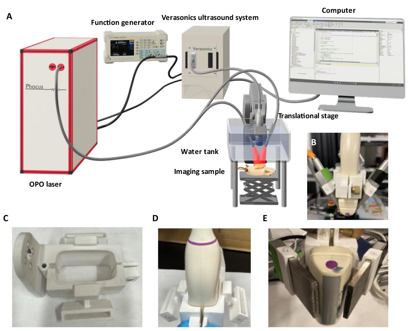
Figure 1. Schematic diagram of a home-built dual-modal photoacoustic and ultrasound localization (PAUL) imaging system. (A) System setup. (B) Front view of the assembly of the linear array transducer and optical fiber housing secured with a custom-made 3D printer holder. (C) Top view of the 3D-printed holder. (D) Linear array transducer inserted into the holder. (E) Optical fiber bundles inserted into both sides of the holder, enabling efficient light delivery for PA imaging.
2. Insert the bifurcated rectangular optical fiber bundles into both sides of the transducer holder to uniformly illuminate the imaging sample from both sides of the linear array transducer (Figure 1E).
3. Secure the transducer holder on an x-y-z translational stage or a robotic arm for precise movement.
4. Connect the transducer to the Verasonics Vantage 256 ultrasound system.
5. Set up a tunable OPO laser source with a wavelength range of 690–950 nm for illumination and configure the laser parameters to a pulse duration of 7 ns and a repetition rate of 10 Hz.
Note: Before each use, measure the laser energy and adjust the fluence to 15 mJ/cm2 to comply with ANSI limits for maximum permissible optical exposure.
6. Attach the trigger-out port of the Verasonics system to the Q-switch input on the laser system (Figure 1A).
7. Connect a function generator to both the flashlamp input of the laser system and the Verasonics trigger-out port (Figure 1A).
8. Set the function generator to provide a trigger signal of a square wave with 10 Hz, 5 Vpp, 2.5 V offset, and 50% duty cycle.
Note: The frequency of the trigger signal should match the repetition rate of the laser system.
9. Program imaging sequences for dual PAUL imaging in the Verasonics Vantage software with MATLAB (a schematic illustration of the data acquisition workflow is shown in Figure 2):
a. Ultrasound imaging: First, apply ultrafast ultrasound imaging with a seven-angle plane-wave transmission (angles from -6° to 6°) to capture 0.5 s of data at a pulse repetition frequency of 500 Hz.
b. PA imaging: Then, perform multi-wavelength PA imaging for 0.2 s at a pulse repetition frequency of 10 Hz, using laser wavelengths of 750 and 850 nm.
c. Set the external Q-switch delay to 290 μs using the “flash2Qdelay” variable in the MATLAB script, per the laser manufacturer’s specifications [16]. The purpose of the “flash2Qdelay” variable in the MATLAB script is to ensure precise synchronization between the flash lamp firing and the Q-switch activation in the laser system. Therefore, the Vantage system can perform data acquisition consistently at the time of laser firing.
Note: Integrate mechanical scanning with the robotic arm in the script if necessary. The Vantage software provides, for example, Verasonics MATLAB scripts, which users can modify for specific purposes.
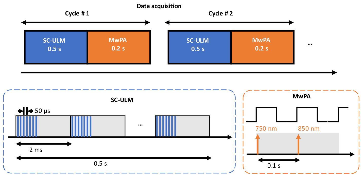
Figure 2. Schematic illustration of the data acquisition workflow for the dual-modal photoacoustic and ultrasound localization (PAUL) imaging system
B. Animal preparation
1. Clean the operating area and prepare all essential supplies.
2. Turn on the heating pad beneath the induction chamber.
3. Connect the oxygen cylinder to the vaporizer and confirm a secure airway connection.
4. Verify that the isoflurane level is within the working range of 1.0%–2.5%.
5. Open the oxygen valve to provide high flow (100% oxygen) and then open the airflow control valve and the anesthesia induction box valve.
6. Set the airflow rate to 2 L/min and adjust the anesthetic concentration to 3%–4%.
7. Place the mouse in the induction chamber and monitor it closely, waiting until it is fully anesthetized (approximately 2–3 min).
8. Turn on the heat pad on the imaging platform.
9. Adjust the airflow control valve to direct the flow from the anesthesia vaporizer to the anesthesia mask on the imaging platform, reducing the anesthetic concentration to 2%.
10. Move the anesthetized mouse from the induction chamber to the imaging platform and secure it with the anesthesia mask.
Note: The mouse's position on the imaging platform can be adjusted as needed to accommodate different imaging scenarios.
11. Apply eye lubricant using a sterile swab, secure the limbs with adhesive tape, and monitor cardiac activity and respiration.
12. Remove the fur from the scanning area using hair removal body cream.
C. In vivo imaging
1. Construct a light- and sound-transparent water tank using a plastic membrane, a 3D-printed frame, and four optical mounting posts.
2. Fill the tank with deionized water to cover half of the tank.
3. Apply a generous amount of ultrasound gel to the mouse's scanning area.
4. Place the water tank on the scanning area and ensure good contact between the ultrasound gel and the tank.
5. Use a 1 mL BD syringe to remove any air bubbles at the gel–tank interface.
6. Place the transducer into the water by adjusting the robotic arm to the starting position.
7. Adjust the water level so the head of the ultrasound transducer is submerged.
8. Turn on the Verasonics ultrasound imaging system and the laser system.
Note: Warm up the laser system 30 min before use and wear laser protection goggles during operation. Warming up the laser before imaging is required to ensure its pulse energy stability.
9. Power on the function generator, confirming that the frequency, peak-to-peak voltage, and offset are as specified in the system setup.
10. In the laser software, set the Q-switch and flashlamp to external trigger mode, and set the laser wavelength to 750 nm.
11. Once the above conditions are met, run the Vantage MATLAB script to initiate real-time ultrasound and PA imaging (Figure 3B).
12. Adjust the transducer position with the robotic arm to locate the optimal imaging plane, guided by the real-time display.
13. Fine-tune the transducer height to maximize PA signal strength from the target region.
14. Once the acquisition position is determined, activate fast laser scan mode in the laser software, setting wavelengths to 750 and 850 nm.
15. Record laser power using the internal power meter in the laser system with the power meter software.
16. Prepare a 1 mL microbubble/PBS solution with a concentration of 1 × 10 particles/mL.
Note: Microbubbles can be synthesized in the lab or purchased commercially.
17. Using a 1 mL syringe with a 31 G × 6 mm needle, draw 100 μL of the microbubble/PBS solution and inject it into the mouse via the tail vein.
Note: Additional contrast agents may be injected for PA imaging depending on the application. For example, indocyanine green (ICG) can be used for PA imaging to visualize lymph nodes.
18. Run the Vantage MATLAB script to continuously acquire UL and PA data.
Note: The total acquisition time or number of cycles depends on the specific application.
19. At the end of the procedure, turn off the vaporizer and place the animal in a recovery cage with heat therapy. Monitor the animal until it is fully mobile, then return it to its home cage.
20. Turn off the Verasonics and laser systems and clean all equipment used in the procedure.
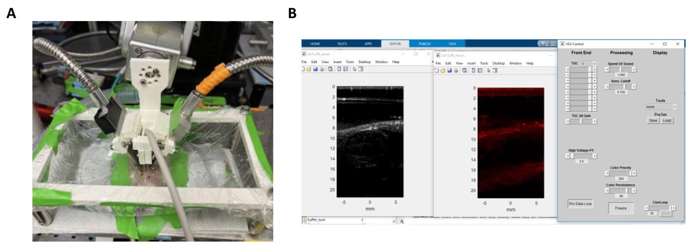
Figure 3. In vivo imaging setup. (A) Snapshot of photoacoustic and ultrasound localization (PAUL) imaging setup for mouse kidney imaging. (B) Verasonics MATLAB interface used for image acquisition and image reconstruction.
Data analysis
This section outlines the reconstruction and processing of both PA and UL imaging, as illustrated in Figure 4.
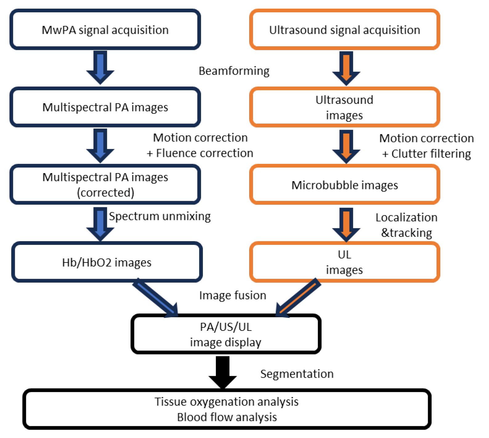
Figure 4. Processing pipeline for photoacoustic (PA) and ultrasound localization (UL) imaging, encompassing data acquisition, image reconstruction, post-processing, and physiological parameter estimation. US: ultrasound.
1. Reconstruct both ultrasound and multi-wavelength PA images offline using the default Verasonics image reconstruction algorithm. The resolution of both the ultrasound and PA imaging setups, including axial and lateral resolution, was characterized using the point spread function (PSF) of a cross-sectional human hair target (Figure 5). The PSF was meticulously analyzed to determine and quantify the resolution of the system. Examples of reconstructed ultrasound and PA images of in vivo kidney regions are shown in Figure 6A and B.
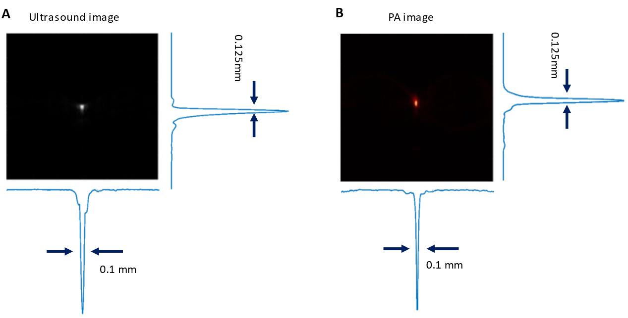
Figure 5. Evaluation of spatial resolution in ultrasound (A) and photoacoustic (PA) imaging (B) using axial and lateral point spread functions (PSF) at the focal zone of a 15.5 MHz linear array transducer
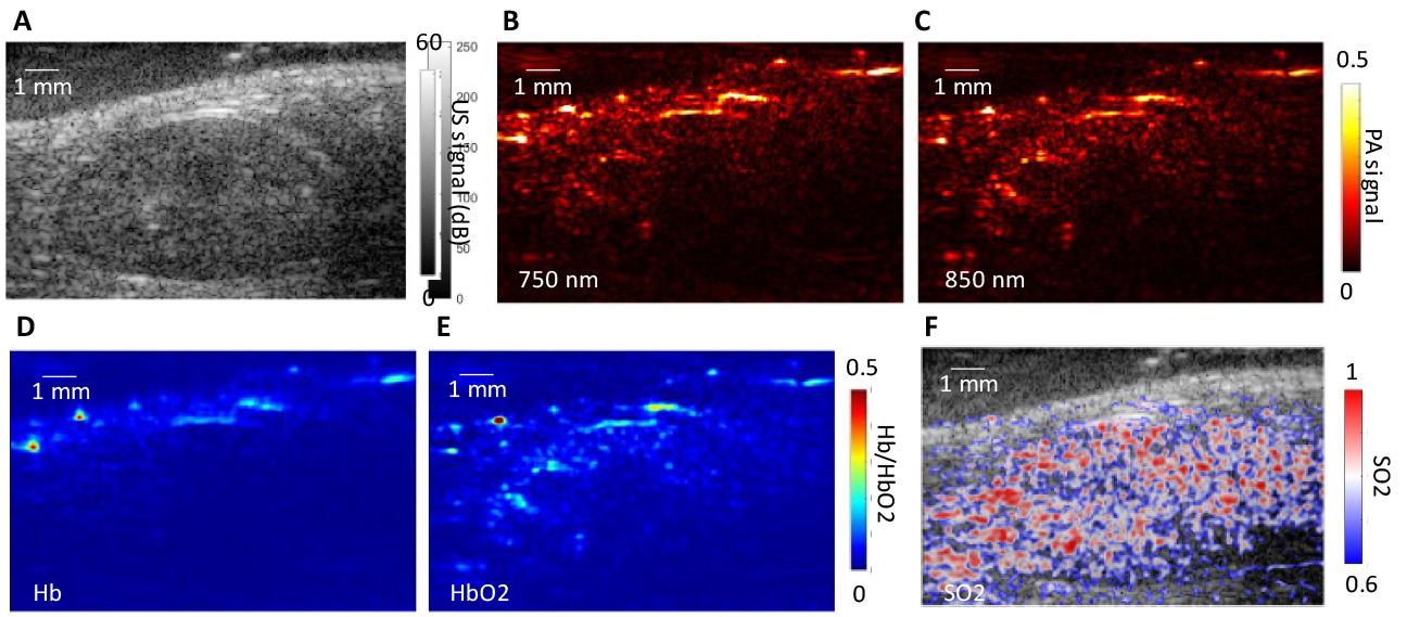
Figure 6. Ultrasound and photoacoustic imaging of a mouse kidney. (A) Ultrasound (US) image shows structural details of the segmented kidney region, while multi-spectral photoacoustic (PA) images at (B) 750 and (C) 850 nm highlight tissue regions with contrast variations. (D, E) Concentrations of deoxygenated hemoglobin (Hb) and oxygenated hemoglobin (HbO2) in a specific region of interest. (F) Distribution of tissue oxygen saturation (SO2) within the kidney region.
2. Select a reference ultrasound image and calculate the normalized frame-to-frame correlation across all ultrasound images to assess respiratory motion and cardiac pulsing (Figure 7).
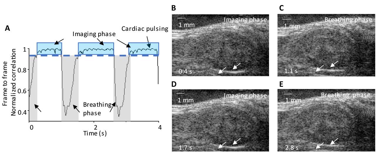
Figure 7. Motion correction in mouse kidney imaging. (A) Identification of three complete breathing cycles, with frame-to-frame correlation analysis from the correlation curve aiding the manual selection of the contributing imaging plane. The identified motions include respiratory (breathing phase) and cardiac pulsing, as indicated by arrows. The imaging phase is indicated by blue windows. (B–E) Consecutive ultrasound images during respiratory and imaging phases at 0.4, 1.1, 1.7, and 2.8 s, respectively. Arrows indicate position changes in the lower boundary of the kidney, highlighting the effects of respiratory motion on tissue displacement during the breathing phase.
3. Among all ultrasound images, discard frames with a correlation coefficient (calculated in step 2) below 0.99, as this indicates significant changes between frames likely caused by breathing motion (Figure 7A). Retain only frames with a correlation coefficient of 0.99 or higher for further processing and analysis (steps 6–12).
4. To account for laser output fluctuations and wavelength-specific power variations, normalize the pixel intensities of each PA image. This can be done by dividing each pixel’s value by the corresponding measured laser energy recorded from the internal power meter of the laser system. Ensure that this normalization process is consistently applied across all frames, including those captured at different wavelengths.
5. Use linear spectral unmixing [4] on the fluence-compensated PA images to extract hemoglobin and deoxyhemoglobin signals. Calculate oxygen saturation as the ratio of hemoglobin signal to total hemoglobin and deoxyhemoglobin signals (Figure 6C, D).
6. Apply spatiotemporal filtering [17] to isolate flowing microbubble signals from the motion-corrected ultrasound images.
7. Apply sparsity constraint (SC) optimization [8] to extract microbubble locations from flowing microbubble signals.
Note: The comparison between the SC and regular localization methods [18] and PSF cross-correlation (PSF-CC) is shown in Figure 8. To implement PSF-CC, after spatiotemporal filtering, a normalized 2D cross-correlation is applied with PSF (Figure 5) to identify microbubbles in each frame.
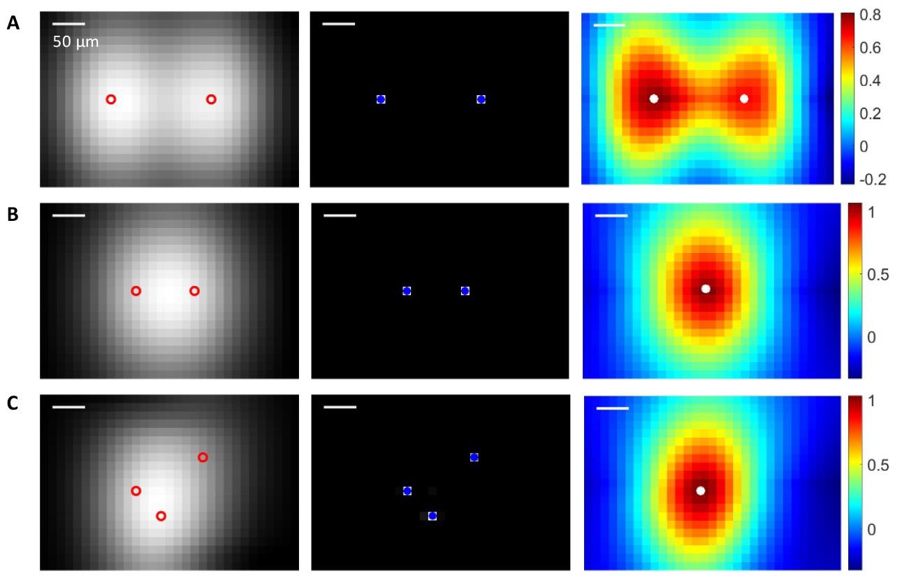
Figure 8. Localization of multiple microbubbles using sparsity constraint (SC) and point spread function cross-correlation (PSF-CC). Left column: Ultrasound images of microbubbles, with red circles indicating the actual positions of the microbubbles. Middle column: Localization image reconstructed via SC optimization, with blue dots marking the recovered microbubble locations using SC. Right column: Normalized cross-correlation map produced by PSF-CC, where white dots indicate the microbubble positions recovered by PSF-CC. The recovered microbubble positions are determined by the positions of the peak coefficients in the map. (A) Two microbubbles are far apart, and both SC and PSF-CC identify all positions. (B) Two microbubbles are close: SC identifies two positions, while PSF-CC retrieves only one. (C) Three microbubbles are close: SC identifies all three positions, while PSF-CC retrieves only one.
8. Track the movement of microbubbles across adjacent frames using a particle tracking algorithm (e.g., simpletracker.m from MathWorks) to discard uncorrelated signals.
9. Accumulate all tracked microbubble traces to create super-resolution frames. Generate a velocity map by calculating the velocity of each microbubble based on trajectory distance and frame intervals. Figure 9A presents a super-resolution image of mouse kidney vasculature.
10. Measure the image resolution of UL imaging using Fourier ring correlation (FRC) [19]. Split the tracking data into two sets, generate two super-resolution images, and calculate the normalized spectral correlation with a 1/2-bit threshold to assess resolution. PA image resolution is evaluated using a wire phantom experiment. Figure 9B shows a kidney super-resolution image with a resolution of 37 μm, a 3-fold improvement over the 105 μm resolution of conventional ultrasound.
11. Calculate the saturation curve of the UL image over acquisition time as the ratio of explored pixels to the total pixels in the region of interest (ROI). Derive the characteristic time from the slope at the origin of the saturation curve. Figure 9C displays super-resolution images at different acquisition times, and Figure 9D shows the saturation curve, indicating a characteristic time of 0.5 s.
12. Fuse PA and UL images for display. Manually segment regions of interest for quantitative analyses, such as tissue oxygenation and blood flow.
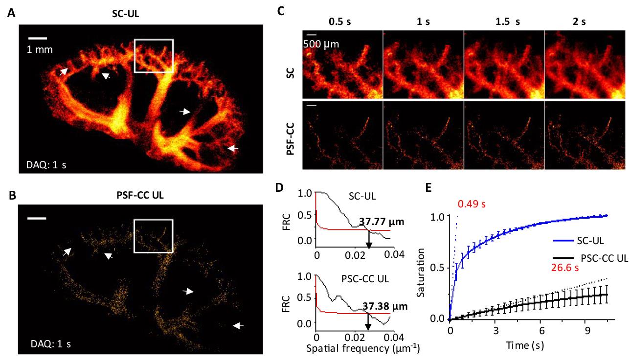
Figure 9. Characterization of ultrasound localization (UL) imaging. (A) UL blood vasculature image reconstructed with sparsity constraint (SC) optimization and with (B) point spread function (PSF) cross-correlation (PSF-CC). The data acquisition time is 1 s. (C) Zoomed-in view of vascular structures at various acquisition times from 0.5 to 2 s. (D) Spatial resolution of SC-UL and PSF-CC UL kidney image with 1 s data acquisition, measured by Fourier ring correlation (FRC). (E) UL image saturation as a function of acquisition times. Adapted from Zhao et al. [8] under the Creative Commons License.
Validation of protocol
This protocol or parts of it has been used and validated in the following research article:
• Zhao et al. [8]. Hybrid photoacoustic and fast super-resolution ultrasound imaging. Nature Communications (Figures 3–6).
To validate our dual-modal fast PAUL imaging protocol for kidney imaging during an oxygen challenge, we performed a series of controlled experiments. We first established the optimal imaging plane for the mouse kidney before microbubble injection and ensured stable transducer positioning. The oxygen challenge was conducted by sequentially altering the inhaled oxygen concentration while continuously acquiring imaging data. Image reconstruction and analysis were performed to quantify deoxygenated and oxygenated hemoglobin levels, as well as absolute blood flow velocity, using predefined regions of interest within the kidney.
The interleaved scanning approach enabled precise frame-to-frame image co-registration, capturing both renal blood speed distribution and renal hemoglobin oxygenation at each oxygen level (Figure 10D). We quantified blood flow velocity and hemoglobin oxygenation in key regions and plotted their changes over time (Figure 10F), showing a positive correlation between blood flow velocity and oxygenation.
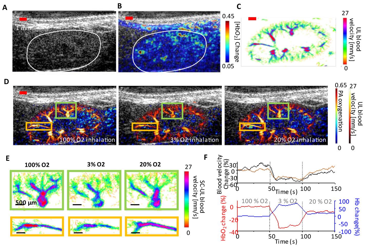
Figure 10. In vivo renal oxygenation and vascular image of a mouse kidney in an oxygen-challenging test. (A) Ultrasound image of a mouse kidney. The kidney is manually identified by the white curve. (B) Oxygenated hemoglobin (HbO2) distribution in a mouse kidney. (C) Blood flow speed map in a mouse kidney. (D) The dual-contrast images show a co-registered photoacoustic (PA) renal oxygenation image and an ultrasound localization (UL) blood speed image under 100%, 3%, and 20% oxygen inhalation. (E) The zoomed-in UL blood flow speed maps represent the highlighted regions in (D) under various levels of oxygen inhalation. (F) Quantitative analysis of the blood speed and HbO2/deoxygenated hemoglobin (Hb) change as a function of time over 150 s of recording. Adapted from Zhao et al. [8] under the Creative Commons License.
General notes and troubleshooting
General notes
1. Ensure that all animal experiments have Institutional Animal Care and Use Committee (IACUC) approval before beginning.
2. The protocol can be adapted for rat imaging as well.
3. Verify that the laser energy used for imaging complies with safety standards. Adjust the laser fluence under 20 mJ/cm2 to meet the ANSI maximum permissible optical exposure limits (American National Standard for Safe Use of Lasers).
4. If using homemade microbubbles, measure both their concentration and size before imaging.
5. For longitudinal imaging requiring continuous microbubble injection, consider using tail vein catheters.
Troubleshooting
Problem 1: The Verasonics system is not responding.
Possible causes: The system may have loose or disconnected cables. The Verasonics license may have expired. An incorrect data acquisition MATLAB code may have been selected.
Solutions: Ensure all system connections are secure and restart the computer. If the license has expired, contact Verasonics support for assistance. Confirm that the correct data acquisition MATLAB code from Verasonics has been selected for your application.
Problem 2: PA signal is not detected.
Possible causes: The laser may not be set to external trigger mode. The function generator might be turned off. The trigger voltage and frequency settings in the function generator may be incorrect. The function generator might not be operating correctly. Input/output triggering ports or connections may be loose or disconnected.
Solutions: Confirm that the laser is set to external trigger mode. Ensure the function generator is turned on. Check that the trigger voltage and frequency are set correctly. Use an oscilloscope to verify the function generator’s operation. Confirm that all input/output triggering ports and connections are secure.
Problem 3: A low number of microbubbles (<50) in each ultrasound frame is detected during localization processing.
Possible causes: The concentration of microbubbles used in the injection may be too low, resulting in insufficient signal for imaging. The imaging duration may exceed the effective circulation time of microbubbles, which typically lasts around 5–10 min.
Solutions: Verify that the microbubble concentration for the injection is adequate. If the concentration is below 10 microbubbles per milliliter, increase it to enhance microbubble signals in the ultrasound images. Check the timing of your imaging. Aim to capture images within 5–10 min post-injection, as signal strength diminishes significantly beyond this period.
Problem 4: The frame discard rate in motion correction is high (>30%).
Possible cause: Excessive respiratory motion may be causing a high frame discard rate during motion correction.
Solutions: Lower the anesthesia level to help reduce respiratory motion artifacts and improve frame retention in the motion correction process.
Acknowledgments
The authors are grateful to Bioacoustics Lab for the ultrasound system. Y-S.C. acknowledges support for this study from 1R01DK138939-01 and the Jump ARCHES endowment through the Health Care Engineering Systems Center. S.Z. acknowledges graduate fellowships from the Beckman Institute. The authors acknowledge their previous work [8] in developing and validating this protocol.
Competing interests
The authors declare no competing interests.
Ethical considerations
All animal experiments were approved by the Institutional Animal Care and Use Committee (IACUC) at the University of Illinois Urbana-Champaign.
References
- Errico, C., Pierre, J., Pezet, S., Desailly, Y., Lenkei, Z., Couture, O. and Tanter, M. (2015). Ultrafast ultrasound localization microscopy for deep super-resolution vascular imaging. Nature. 527(7579): 499–502. https://doi.org/10.1038/nature16066
- Heiles, B., Chavignon, A., Hingot, V., Lopez, P., Teston, E. and Couture, O. (2022). Performance benchmarking of microbubble-localization algorithms for ultrasound localization microscopy. Nat Biomed Eng. 6(5): 605–616. https://doi.org/10.1038/s41551-021-00824-8
- Wang, L. V. and Yao, J. (2016). A practical guide to photoacoustic tomography in the life sciences. Nat Methods. 13(8): 627–638. https://doi.org/10.1038/nmeth.3925
- Li, M., Tang, Y. and Yao, J. (2018). Photoacoustic tomography of blood oxygenation: A mini review. Photoacoustics. 10: 65–73. https://doi.org/10.1016/j.pacs.2018.05.001
- Zhao, S., Lee, L., Zhao, Y., Liang, N. C. and Chen, Y. S. (2023). Photoacoustic signal enhancement in dual-contrast gastrin-releasing peptide receptor-targeted nanobubbles. Front Bioeng Biotechnol. 11: e1102651. https://doi.org/10.3389/fbioe.2023.1102651
- Weber, J., Beard, P. C. and Bohndiek, S. E. (2016). Contrast agents for molecular photoacoustic imaging. Nat Methods. 13(8): 639–650. https://doi.org/10.1038/nmeth.3929
- Omar, M., Aguirre, J. and Ntziachristos, V. (2019). Optoacoustic mesoscopy for biomedicine. Nat Biomed Eng. 3(5): 354–370. https://doi.org/10.1038/s41551-019-0377-4
- Zhao, S., Hartanto, J., Joseph, R., Wu, C. H., Zhao, Y. and Chen, Y. S. (2023). Hybrid photoacoustic and fast super-resolution ultrasound imaging. Nat Commun. 14(1): 2191. https://doi.org/10.1038/s41467-023-37680-w
- Chen, H., Mirg, S., Gaddale, P., Agrawal, S., Li, M., Nguyen, V., Xu, T., Li, Q., Liu, J., Tu, W., et al. (2023). Dissecting Multiparametric Cerebral Hemodynamics using Integrated Ultrafast Ultrasound and Multispectral Photoacoustic Imaging. bioRxiv: e566048. https://doi.org/10.1101/2023.11.07.566048
- Tang, Y., Wang, N., Dong, Z., Lowerison, M., del Aguila, A., Johnston, N., Vu, T., Ma, C., Xu, Y., Yang, W., et al. (2025). Non-Invasive Deep-Brain Imaging With 3D Integrated Photoacoustic Tomography and Ultrasound Localization Microscopy (3D-PAULM). IEEE Trans Med Imaging. 44(2): 994–1004. https://doi.org/10.1109/tmi.2024.3477317
- Chen, Y. S., Zhao, S., Basu, S., Shi, J., Song, K., Siripun, P., Huynh, H., Zhao, Y. and Campbell, R. (2024). Whole-brain functional photoacoustic/ultrasound localization (PAUL) imaging for monitoring blood-brain barrier modulation. Res Squ: ers–4754944/v1. https://doi.org/10.21203/rs.3.rs-4754944/v1
- Chen, Q., Yu, J., Rush, B. M., Stocker, S. D., Tan, R. J. and Kim, K. (2020). Ultrasound super-resolution imaging provides a noninvasive assessment of renal microvasculature changes during mouse acute kidney injury. Kidney Int. 98(2): 355–365. https://doi.org/10.1016/j.kint.2020.02.011
- Zhang, W., Cai, F., Xu, H., Wu, Y., Yu, X. a., Sun, L., Zhang, T., Yu, B. Y., Zheng, X., Tian, J., et al. (2022). Small-Molecule Photoacoustic Imaging Probe with Aggregation-Enhanced Amplitude for Real-Time Visualization of Acute Kidney Injury. Anal Chem. 94(27): 9697–9705. https://doi.org/10.1021/acs.analchem.2c01106
- Porte, C., Lisson, T., Kohlen, M., von Maltzahn, F., Dencks, S., von Stillfried, S., Piepenbrock, M., Rix, A., Dasgupta, A., Koczera, P., et al. (2024). Ultrasound Localization Microscopy for Breast Cancer Imaging in Patients: Protocol Optimization and Comparison with Shear Wave Elastography. Ultrasound Med Biol. 50(1): 57–66. https://doi.org/10.1016/j.ultrasmedbio.2023.09.001
- Kratkiewicz, K., Pattyn, A., Alijabbari, N. and Mehrmohammadi, M. (2022). Ultrasound and Photoacoustic Imaging of Breast Cancer: Clinical Systems, Challenges, and Future Outlook. J Clin Med. 11(5): 1165. https://doi.org/10.3390/jcm11051165
- Kratkiewicz, K., Manwar, R., Zhou, Y., Mozaffarzadeh, M. and Avanaki, K. (2021). Technical considerations in the Verasonics research ultrasound platform for developing a photoacoustic imaging system. Biomed Opt Express. 12(2): 1050–1084. https://doi.org/10.1364/boe.415481
- Demene, C., Deffieux, T., Pernot, M., Osmanski, B. F., Biran, V., Gennisson, J. L., Sieu, L. A., Bergel, A., Franqui, S., Correas, J. M., et al. (2015). Spatiotemporal Clutter Filtering of Ultrafast Ultrasound Data Highly Increases Doppler and fUltrasound Sensitivity. IEEE Trans Med Imaging. 34(11): 2271–2285. https://doi.org/10.1109/tmi.2015.2428634
- Song, P., Trzasko, J. D., Manduca, A., Huang, R., Kadirvel, R., Kallmes, D. F. and Chen, S. (2018). Improved Super-Resolution Ultrasound Microvessel Imaging With Spatiotemporal Nonlocal Means Filtering and Bipartite Graph-Based Microbubble Tracking. IEEE Trans Ultrason Ferroelectr Freq Control. 65(2): 149–167. https://doi.org/10.1109/tuffc.2017.2778941
- Hingot, V., Chavignon, A., Heiles, B. and Couture, O. (2021). Measuring Image Resolution in Ultrasound Localization Microscopy. IEEE Trans Med Imaging. 40(12): 3812–3819. https://doi.org/10.1109/tmi.2021.3097150
Article Information
Publication history
Received: Nov 14, 2024
Accepted: Feb 7, 2025
Available online: Mar 6, 2025
Published: Mar 20, 2025
Copyright
© 2025 The Author(s); This is an open access article under the CC BY-NC license (https://creativecommons.org/licenses/by-nc/4.0/).
How to cite
Zhao, S., Paul, S., Yi, J. and Chen, Y. S. (2025). Dual-Modal Fast Photoacoustic/Ultrasound Localization Imaging with Sparsity-Constrained Optimization. Bio-protocol 15(6): e5247. DOI: 10.21769/BioProtoc.5247.
Category
Biological Engineering > Biomedical engineering
Biophysics > Microscopy
Biological Sciences
Do you have any questions about this protocol?
Post your question to gather feedback from the community. We will also invite the authors of this article to respond.