- Protocols

- Articles and Issues
- For Authors
- About
- Become a Reviewer

HS–GC–MS Method for the Diagnosis of IBD Dynamics in a Model of DSS-Induced Colitis
(*contributed equally to this work) Published: Vol 15, Iss 6, Mar 20, 2025 DOI: 10.21769/BioProtoc.5246 Views: 3165
Reviewed by: Marco Di GioiaElke M. MuntjewerffAnonymous reviewer(s)
Original research article
The authors used this protocol in:
Mar 2024
Advertisement


Protocol Collections
Comprehensive collections of detailed, peer-reviewed protocols focusing on specific topics


Related protocols

Abstract
Inflammatory bowel disease (IBD) is highly prevalent globally and, in the majority of cases, remains asymptomatic during its initial stages. The gastrointestinal microbiota secretes volatile organic compounds (VOCs), and their composition alters in IBD. The examination of VOCs could prove beneficial in complementing diagnostic techniques to facilitate the early identification of IBD risk. In this protocol, a model of sodium dextran sulfate (DSS)-induced colitis in rats was successfully implemented for the non-invasive metabolomic assessment of different stages of inflammation. Headspace–gas chromatography–mass spectrometry (HS–GC–MS) was used as a non-invasive method for inflammation assessment at early and remission stages. The disease activity index (DAI) and histological method were employed to assess intestinal inflammation. The HS–GC–MS method demonstrated high sensitivity to intestine inflammation, confirmed by DAI and histology assay, in the acute and remission stages, identifying changes in the relative content of VOCs in stools. HS–GC–MS may be a useful and non-invasive method for IBD diagnostics and therapy effectiveness control.
Key features
• Experiments performed in vivo to better control DSS-induced colon damage and to aid the study of IBD development in humans.
• Optimized for the following organisms: Wistar rats and C57BL/6 mice.
• An easily assessed disease activity index (DAI) (weight loss, stool consistency, degree of fecal occult blood) and histopathological examination are suggested for additional IBD confirmation.
• Enables VOC testing with relatively small stool samples.
Keywords: Headspace–gas chromatography–mass spectrometry (HS–GC–MS)Graphical overview
Background
Inflammatory bowel diseases (IBD) are a significant challenge in gastroenterology [1]. Diagnosing these diseases is difficult, and reliable early diagnosis is still a challenge. Severe IBD symptoms such as bloody diarrhea can debilitate or even lead to death. IBD diagnostic techniques can also cause complications (functional impairment, pain reactions, and bacterial infections) [2]. It is therefore vital to identify alternative, safe, and rapid molecular methods of diagnosis and treatment.
Microorganisms secrete volatile organic compounds (VOCs), including short-chain fatty acids, that constitute the principal metabolites of the microbiota in the colon [3,4]. In particular, acetic, propionic, and butyric acids produced by the microbiota account for 90%–95% of VOCs in the colon (ratio 3:1:1) [5]. Other volatile metabolites include medium- and long-chain fatty acids or amino acid derivatives. The ratio of VOC components in samples is correlated with the stage of intestinal inflammation [6,7]. Fecal VOC analysis represents a non-invasive diagnostic method for differentiating IBD, including ulcerative colitis (UC) and Crohn's disease (CD). Some studies have demonstrated that specific VOCs are elevated in patients with active CD, with concentrations returning to normal levels following treatment. The analysis of VOCs is conducted through the use of gas chromatography combined with mass spectrometry (GC–MS) [8,9]. This method enables the comparison of biological samples, including fecal, through the use of the vapor-phase extraction technique [10]. The use of experimental animal models enables the efficacy of the method to be demonstrated at various stages of the inflammatory process.
The most accurate models for IBD research include trinitrobenzene sulfonic acid (TNBS), oxazolone, and sodium dextran sulfate (DSS) treatment. The TNBS model induces colitis as a consequence of a Th1-mediated immune response, whereas oxazolone induces colitis with a Th2-type cytokine response. The DSS model is the most commonly used for modeling colitis in rodents, facilitating the study of innate immunity and healing processes [1,11–15]. However, DSS has been demonstrated to cause damage to the colonic epithelium and to alter the intestinal microbiota and its metabolites [16,17]. It has been suggested that shifts in the microbiota with subsequent changes in metabolites are a consequence of the formation of colitis [18].
In this study, we pursued the goal of establishing a protocol for the analysis of acute and remission stages of intestine inflammation using the HS–GC–MS method. The approach was demonstrated in DSS-induced colitis in rats. Intestinal inflammation was confirmed by histological examination and evaluation of a disease activity index.
Materials and reagents
The following materials and equipment are recommended for this protocol, but alternatives from other sources can also be used when proven to be equivalent.
Biological materials
In the experiment, we used female, 2-month-old Wistar rats (200–230 g). You can also use 2-month-old male Wistar rats.
Note: This protocol can also be used for C57BL/6 male and female mice (20–25 g) but with a lower concentration of DSS (3%).
Reagents
1. Food and water for rats (Laboratorcorm, lot not available)
2. Dextran sulfate sodium salt (DSS), MW ca. 40,000, powder (Alfa Aesar, catalog number: 61701051)
3. Potassium dihydrogen orthophosphate (CDH, catalog number: 821123)
4. Ammonium sulfate (NeoFroxx Gmbh 1333KG001, catalog number: 62E1113f)
5. Ultra-high purity helium (99.9999%)
6. Paraffin wax Histomix Extra (BioVitrum, catalog number: 10342)
7. Hematoxylin (BioVitrum, catalog number: 05-002/М)
8. Eosin (BioVitrum, catalog number: 05-011)
9. Histological mounting medium Vitrogel (BioVitrum, catalog number: HM-VI-A250)
10. 10% buffered formalin, pH 7.0–7.8 (BioVitrum, catalog number: B06-001/M)
11. Isopropyl alcohol (Chimmed, catalog number: 00000006997)
12. O-xylene (Chimmed, catalog number: 95662-2.5L)
13. Phosphate-buffered saline (PBS) (VWR International LLC, catalog number: 18G2056770)
Solutions
1. Liquid 4.5% DSS (see Recipes)
2. Liquid PBS (see Recipes)
Recipes
1. Liquid 4.5% DSS
Dissolve 4.5 g of DSS powder in 100 mL of water
2. Liquid PBS
Add one tablet in 100 mL of distilled water
Laboratory supplies
1. Stool collection tubes (1.5 mL Eppendorf)
2. Euthanasia equipment: Guillotine, chloroform
3. Surgical instruments:
a. Scissors pointed straight 165 mm (Dealmed, catalog number: J-22-022)
b. Anatomical forceps 250 mm (Dealmed, catalog number: J-16-026)
c. Surgical forceps 200 mm (Dealmed, catalog number: J-16-034)
d. Anatomical forceps, curved (Dealmed, catalog number: 37-614)
e. Straight pointed anatomical forceps (Dealmed, catalog number: 12-560-00-07)
f. Microsurgical scissors (Dealmed, catalog number: MS-1204)
g. Eye scissors for suture removal (Dealmed, catalog number: J-22-180A)
4. Sewing thread
5. Toothpicks
6. Pipettes (20, 200, and 1,000 μL) (Gilson, catalog number: F167300)
7. Microtome blades R35, Japan (Feather, catalog number: 253740)
8. Labeled histological cassettes (BioVitrum, catalog number: Kg-07)
9. 10 mL clear headspace screw vials (Gluvex D22.5xH50 p/n SLV 101M, catalog number: 201250800)
10. Screw magnetic cap and septa match with SLV 101M (Gluvex SLV10/20SCM, catalog number: 211225213)
Equipment
1. Rat cages and drinkers 545 mm × 395 mm × 200 mm (Laboratorcorm, catalog number: Т-4\1)
2. Scales
3. Gas chromatography–mass spectrometry (GC–MS) system (Shimadzu, model: GCMS-QP2010) with a headspace (HS) extractor (Shimadzu, model: HS-20)
4. VFWAX MS column with 30 m length, 0.25 mm diameter, and 0.25 μm phase thickness (Agilent technologies, catalog number: CP9205)
5. Rotary microtome (Thermo Scientific, model: Thermo HM 340E)
6. Slice transfer system (Thermo, model: STS)
7. Light microscopy (Zeiss, model: Primo Star)
8. Histological embedding workstation (Thermo Fisher Scientific, model: HistoStar 12587976)
Software and datasets
1. GCMS solution (version 2.45, Shimadzu Corporation)
2. NIST 14 mass spectral libraries (National Institute of Standards and Technology http://www.nist.gov/) with automated mass spectral deconvolution and identification system (AMDIS version 2.72)
Procedure
A. Modeling of colitis and collection of fecal samples
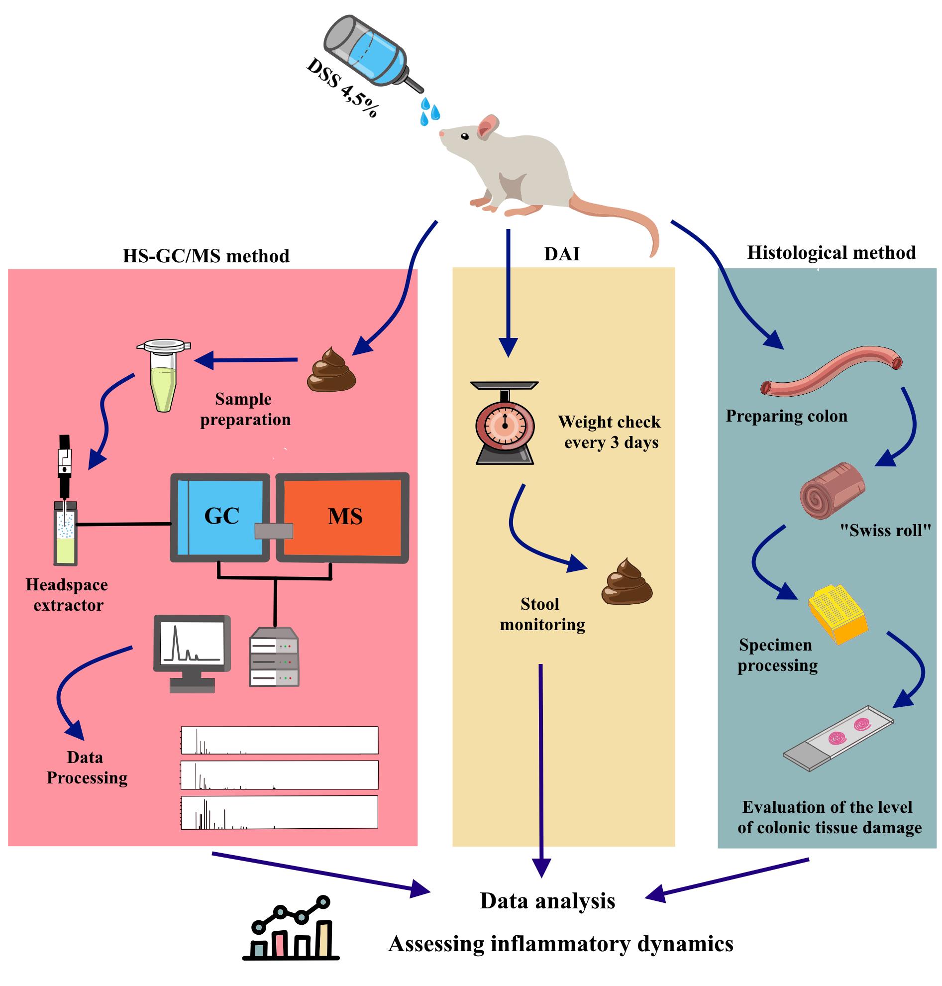
1. Randomly divide the rats into three groups: control group, sodium dextran sulfate group for 7 days (DSS7), and DSS group for 14 days (DSS14). According to our general workflow (Figure 1), both the DSS7 and DSS14 groups drink DSS solution for the first 7 days; the control group is given pure water. All solutions are administered using drinkers. After 7 days, the DSS7 group is euthanized. The DSS14 group proceeds to recovery without DSS solution for the following 7 days.
2. Prepare a liquid solution of 4.5% DSS for the two groups (DSS7 and DSS14) and pure water for the control group.
3. Assign an identification number to each animal.
4. Prepare a table to record weight and condition data for the disease activity index (DAI).
5. On the first day of the experiment, weigh, record, and collect a fecal sample from each animal.
6. Store stool samples at -20 °C.
7. Every 3 days, collect stool samples from all animals and record the condition of each animal to estimate DAI.
Note: An overview of the modeling of colitis and collection of fecal samples can be found in Figure 1.
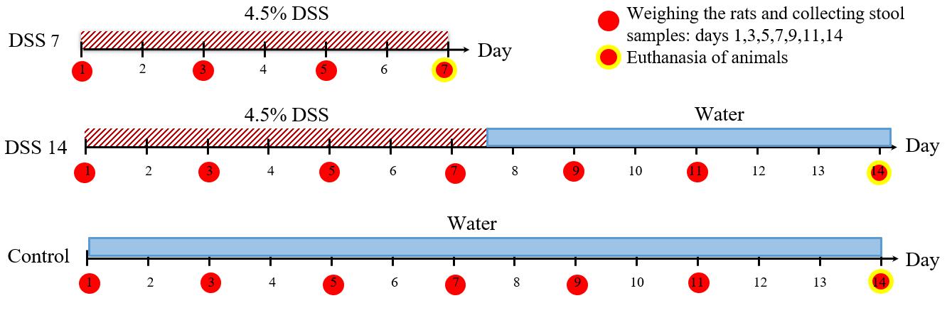
Figure 1. General workflow for colitis modelling, stool sampling, and rat euthanasia
B. Clinical disease score
1. Estimate the DAI of the rats by scoring body weight loss, stool consistency, and degree of stool occult blood (Table 1, Figure 2).
Table 1. Disease activity index (DAI) scores
| Score | Body weight loss | Stool consistency | Degree of stool occult blood |
| 0 | <1% | Formed (#1*) | Normal color stool |
| 1 | 1%–5% | Soft (#2*) | |
| 2 | 5%–10% | Watery stool (#3*) | Reddish color stool |
| 3 | 10%–15% | ||
| 4 | >15% |
*see Figure 2 for visual examples.
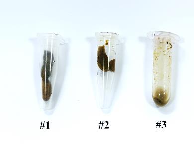
Figure 2. Examples of three different types of rat stools
2. Monitor the DAI daily to assess disease severity (Figure 3).
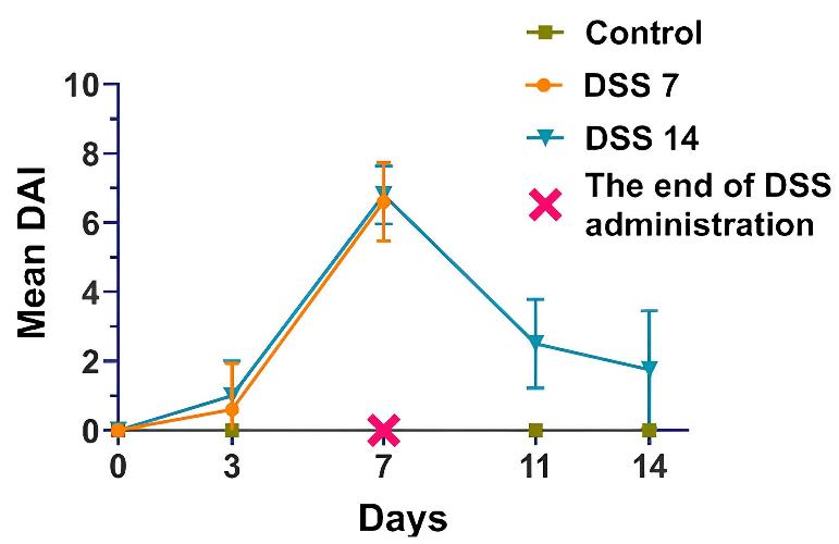
Figure 3. Dynamics of the disease activity index (DAI) in each group
C. Preparing colon animals for histology
1. Euthanize animals with chloroform and subsequent decapitation.
2. Wet the animal skin with water to maintain the hair out of the way.
3. Make a tray with paraffin wax. Put the animal on the paraffin. Spread the limbs apart and pin them (Figure 4A).
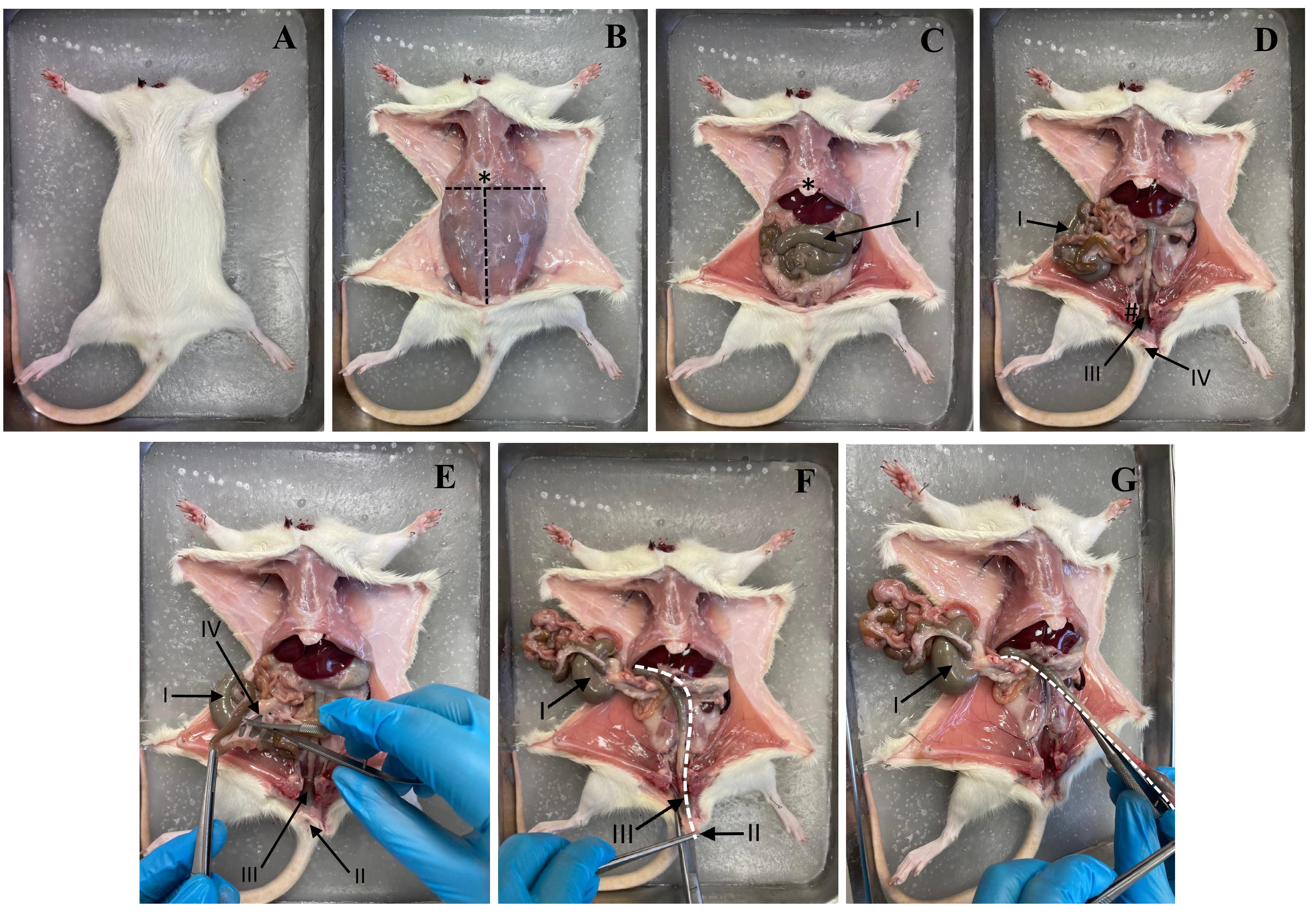
Figure 4. Stages of rat dissection. (A) Fixing the rat on the plate. (B) Skin incision and fixation of the skin flaps. (C) Opening of the abdominal cavity. (D) Visualization of the intestine. (E) Incision of the mesentery. (F) Improvement of access to the colon. (G) Extraction of the colon. Dotted line: cutting line. * Xiphoid process. I: Caecum. II: Anus. III: Rectum. IV: Mesentery.
4. Use forceps (#2 in Figure 5) to lift the skin and make a small incision with scissors (#1 in Figure 5), running left to right. Use scissors (#1 in Figure 5) to separate the skin from the muscle. Insert scissors under the skin and separate the skin and fat from the muscle. Pull the skin to the sides and secure with pins. See Figure 4B.
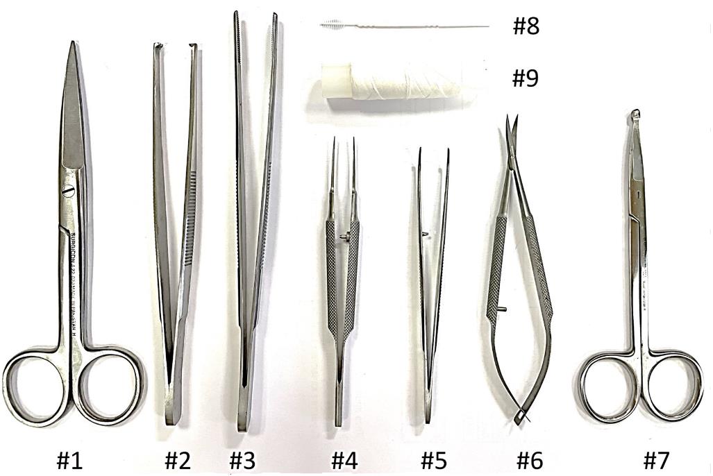
Figure 5. Fine surgical tools for preparing animal colons for histology for the Swiss roll technique
5. Make a midline incision with scissors (#1 in Figure 5) from the chest to the pubic area. Pull the abdominal walls apart and pin them in place (Figure 4C and D).
6. Cut the mesentery to remove the colon. Remove the colon from the anus to the cecum with scissors (#6 in Figure 5) (Figure 4E–G).
7. Rinse the colon with PBS solution. Hold the cecum with forceps (#5 in Figure 5) and insert the PBS solution needle into the small intestine. Clamp the needle to the cecum with forceps and inject the PBS solution. See Figure 6A–C.
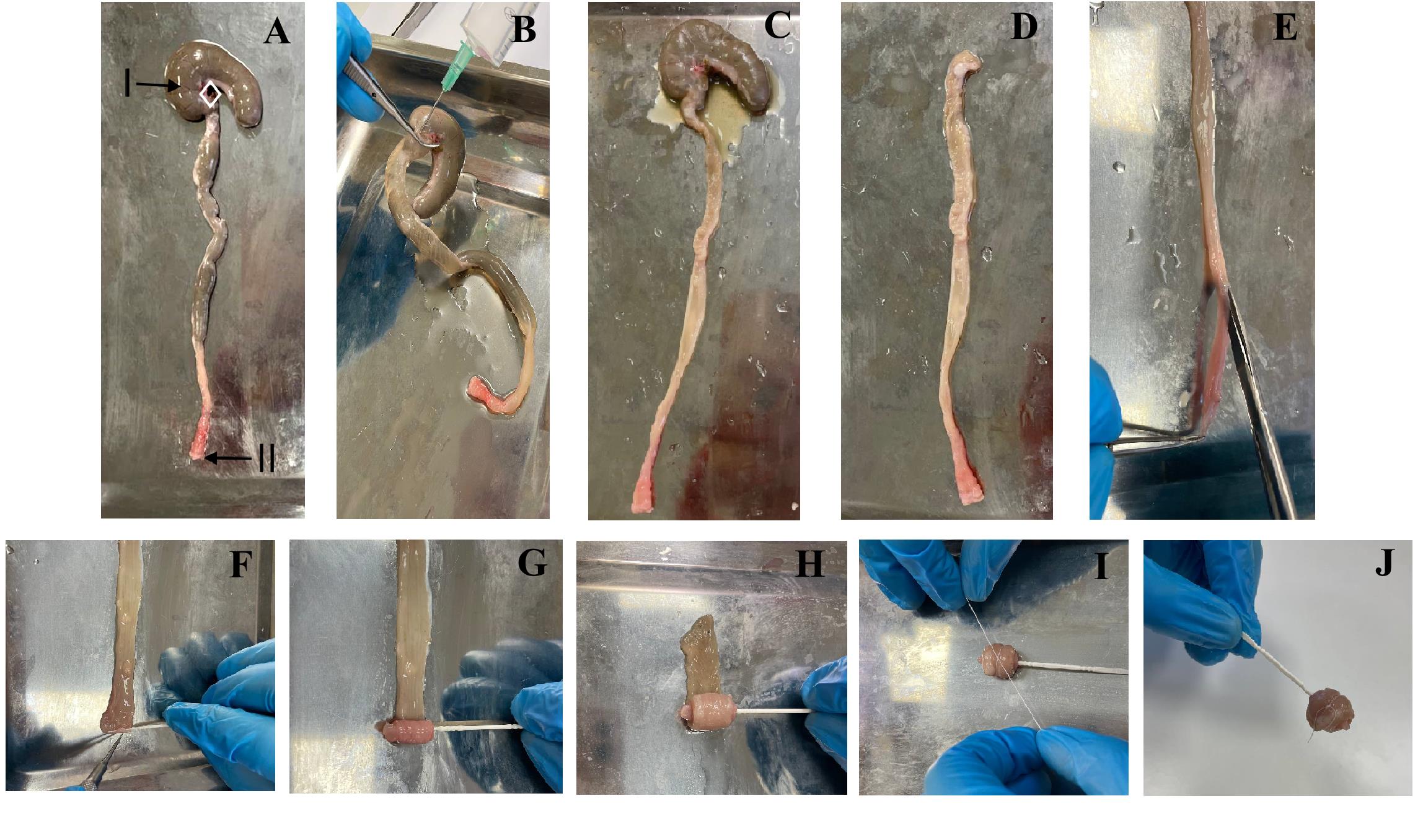
Figure 6. Preparing animal colons for histology with the Swiss roll technique. (A) Isolated colon (I: cecum; II: anus). (B) Colonic fecal cleansing. (C) Cleaned colon. (D) Colon without the cecum. (E) Colon dissection. (F) Fixing a toothpick to the anus. (G) Starting to make a roll. (H) Finishing the roll. (I) Fixing the roll with sewing thread. (J) Finished Swiss roll.
8. Cut off the cecum (Figure 6D).
9. Put the colon on a flat surface. Open the colon from the end with scissors. Wet the colon with PBS solution and remove any remaining fecal matter (Figure 6E, F).
10. Place the colon flat on a clean surface. Twist the colon using the Swiss roll method. Hook the rectum with a toothpick. Thread the colon onto the toothpick. Tie the colon roll with a thin string. See Figure 6G–J.
11. Place the Swiss roll in a container with formalin.
D. Histology
1. Remove the specimen after 48 h of fixation in formalin.
2. Label the histological cassette according to the specimen list and the code on the fixative container.
3. Place a plastic insert with a hole of appropriate diameter into the histology cassette (Figure 7).
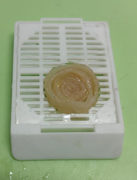
Figure 7. Histological cassette with an insert that fixes the specimen
4. Carefully remove the toothpick from the center of the Swiss roll using tweezers.
5. Place the specimen in the histology cassette so that it does not touch the edges of the hole in the plastic insert and lies flat on its side.
6. Cut off excess specimens with a knife using the sharp blade of a disposable scalpel or microtome knife to remove any protruding parts above the surface of the plastic insert.
7. Cut the Swiss roll thread in two places and remove the fragments with tweezers.
8. Close the lid of the histology cassette and place it in fixative to prevent drying.
9. Perform the histological slide preparation according to the protocol for large materials shown in Table 2.
Table 2. Protocol specimen processing
| No. | Reagent | Temperature (°С) | Time (min) |
| 1 | Isopropyl alcohol | 18–22 | 50 |
| 2 | Isopropyl alcohol | 18–22 | 50 |
| 3 | Isopropyl alcohol | 18–22 | 50 |
| 4 | Isopropyl alcohol | 18–22 | 50 |
| 5 | Isopropyl alcohol | 18–22 | 50 |
| 6 | O-xylene | 18–22 | 50 |
| 7 | O-xylene | 18–22 | 50 |
| 8 | Paraffin wax Histomix Extra | 62 | 60 |
| 9 | Paraffin wax Histomix Extra | 62 | 60 |
10. Use a histological embedding workstation. Fill the histological block so that the flat side of the specimen is on the surface of the pouring mold.
11. Use the rotary microtome with the slice transfer system and microtome blades. Cut 3.5 μm thick sections and put them on labeled slides, with two sections per slide.
12. Dry the slides vertically in a stream of air for at least 24 h.
13. Stain the specimens with hematoxylin/eosin according to Table 3.
Table 3. Staining of samples
| No. | Reagent | Time (min) |
| 1 | O-xylene | 5 |
| 2 | O-xylene | 5 |
| 3 | Isopropyl alcohol | 3 |
| 4 | Isopropyl alcohol | 3 |
| 5 | Distilled water | 5 |
| 6 | Distilled water | 5 |
| 7 | Hematoxylin | 7 |
| 8 | Distilled water | 5 |
| 9 | Distilled water | 5 |
| 10 | Eosin | 40 |
| 11 | Distilled water | 5 |
| 12 | Distilled water | 5 |
| 13 | Isopropyl alcohol | 3 |
| 14 | Isopropyl alcohol | 3 |
| 15 | O-xylene | 5 |
| 16 | O-xylene | 5 |
14. Use a histological mounting medium Vitrogel, place the slides under a coverslip, and dry horizontally for at least 24 h.
15. Examine the specimens under a light microscope at 100× and 400× magnification. Take the microphotographs you need.
16. Use a scoring system (Table 4, Figure 8) to evaluate colon damage. Take into account the thickness of the mucosa, the preservation of its structure, the presence and location of crypt abscesses, the foci of mucosal destruction, the infiltration by immune cells, the presence of lymphoid accumulations in the submucosal layer, the number of goblet cells, and any other possible abnormalities.
Table 4. Scoring criteria for histological lesions in the colon. The protocol described here was based on previous works [18].
| Content | Score | ||||
| 0 | 1 | 2 | 3 | 4 | |
| Goblet cells | No loss | Mild loss | Moderate loss | Severe loss | |
| Mucosal thickness | No change | Mild thickening | Moderate thickening | Severe thickening | |
| Inflammatory cells | No infiltration | Mild increase | Moderate increase | Severe increase | |
| Submucosal inflammatory cell infiltration | No infiltration | - | Mild increase | Moderate increase | Severe increase |
| Destruction of architecture | No damage | - | - | Mild destruction | Moderate destruction |
| Crypt abscesses | 0 | 1–3 | 4–6 | 7–9 | >10 |
Notes:
1. Example of scoring according to Figure 9.
2. For example, DSS7 in Figure 9 clearly shows swelling of the submucosa, loss of goblet cells, infiltration of the mucosa and submucosa by immune cells, and disruption of the mucosal structure. In the case of a significant extent of damage, we assign 4 points. DSS14 shows the accumulation of lymphoid cells in the submucosal layer and infiltration of the mucosa and submucosa with immune cells, as well as a decrease in the number of goblet cells and moderate disruption of the mucosa structure.
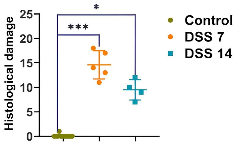
Figure 8. Histopathological evaluation of the colon of each group of rats. Data are presented as individual means or mean ± SD for each group. *p < 0.025; ***p < 0.0005.
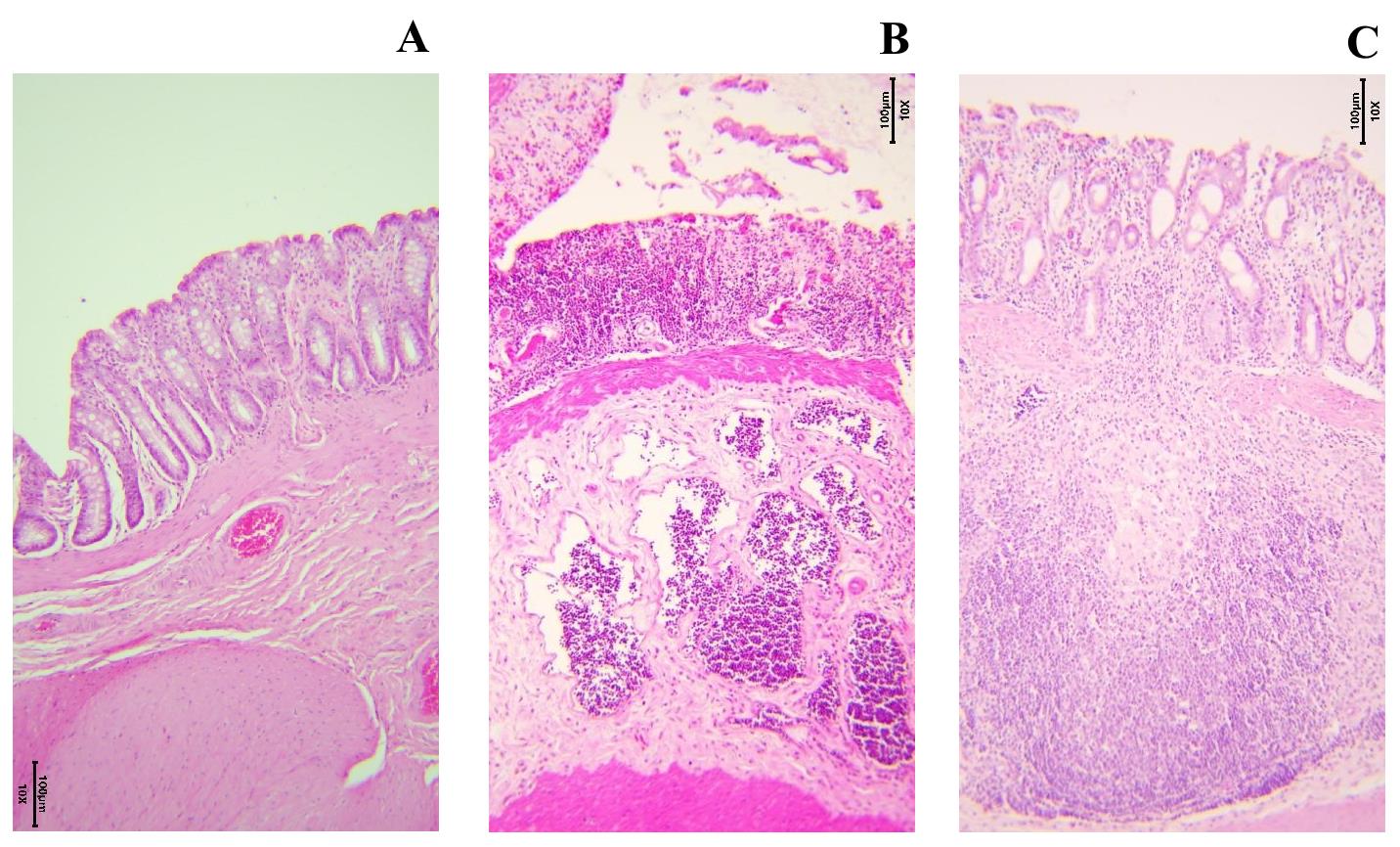
Figure 9. Colon tissue stained with H&E (10×) in different phases of inflammation. (A) Healthy colon wall of a control-group rat. (B) Damaged rat colon from the DSS7 group. Disturbed mucosal architecture, isolated goblet cells, and marked inflammatory infiltration. (C) Rat colon from the DSS14 group. Signs of restoration of the mucosal architecture and appearance of crypts.
17. Prepare a description of the specimens and accompanying photographs for future reference (Figure 9).
E. Gas chromatography–mass spectrometry (GC–MS) headspace extraction
Note: An overview of the device and GC–MS process can be found in Figure 10.
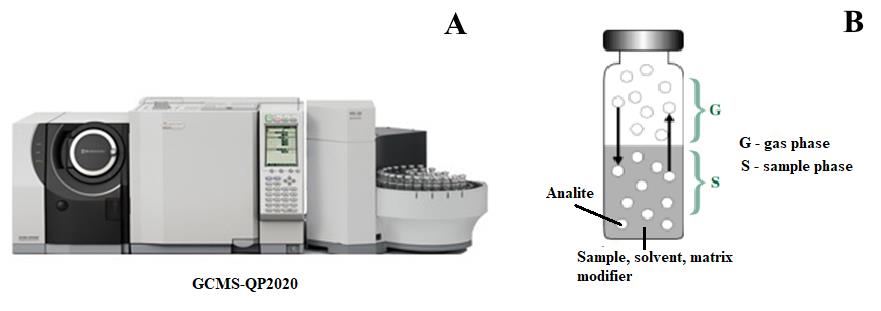
Figure 10. GCMS-QP2020 device and GC–MS process. (A) Gas chromatography–mass spectrometry equipment. (B) Gas phase formation reaction from the sample.
1. Place 50–100 mg of stool samples and 500 μL of water samples in 10 mL screw-capped tubes for the Shimadzu HS-20 headspace extractor.
2. Add a total of 0.2 g of salt mixture (ammonium sulfate and potassium dihydrogen orthophosphate in a 4:1 ratio) to increase the ionic strength of the solution.
3. Set the temperature of the headspace extractor oven to 80 °C, the temperature of the sample line to 220 °C, the temperature of the transfer line to 220 °C, the equilibration time to 15 min, the pressurization time to 2 min, the loading time to 0.5 min, the injection time to 1 min, and the needle rinsing time to 7 min.
4. Seal vials and analyze on a Shimadzu QP2010 Ultra GC/MS with a Shimadzu HS-20 headspace extractor and a VFWAX MS column (30 m length, 0.25 mm diameter, and 0.25 μm phase thickness).
5. Set the initial column temperature to 80 °C, heating rate from 20 °C/min to 240 °C, and exposure time of 20 min.
6. The carrier gas should be helium 99.9999%, the injection mode should be splitless, and the flow rate should be 1 mL/min. The ion source temperature must be 230 °C. The interface temperature must be 240 °C.
7. Use the total ion current (TIC) monitoring mode.
8. To analyze the obtained mass spectra, use the NIST 14 mass spectra library with automated mass spectral deconvolution and identification system (AMDIS version 2.72) (Figure 11).
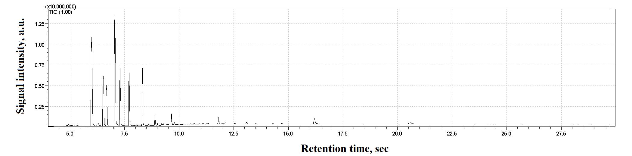
Figure 11. Examples of GC–MS spectra of a stool sample
Data analysis
A. Data processing
The HS–GC–MS data can be processed as follows:
1. Transform the data into relative abundances by calculating the peak areas for the selected compounds using the AMDIS software.
2. Estimate the percentage of volatile compounds in each sample by summing the percentage of confidently identified compounds in the AMDIS database for each sample.
3. Subsequently, the resulting values must be recalculated as a percentage of the total reliably identified compounds. These conversions are necessary to circumvent content estimation errors due to unreliable matrix signals caused by noise.
4. For subsequent analysis, the relative quantitative content of each metabolite in the sample must be calculated. By “relative quantitative content”, we mean a comparison of the intensities of the studied metabolites normalized to the total ion current.
5. Calculate the relative intensity as follows:
where Irel is the relative intensity of the metabolite, Imet is the intensity of the metabolite (magnitude of the ion current for the given metabolite), and ΣI is the intensity of all analyzed metabolites (magnitude of the total ion current).
B. Statistical analysis
1. For each metabolite, calculate the percentage of samples in which it was detected.
It should be noted that for the purposes of further statistical analysis, 21 metabolites were selected, each of which was present in over 60% of all samples in the experiment. Table 5 presents the obtained values for the stable, detected metabolites in the DSS group across all experimental days, for the control group, and for all groups combined. Figure 12 presents a heatmap of the average concentration levels (on a logarithmic scale) of these metabolites across the groups.
Table 5. List of 21 stable, detected metabolites
| Metabolites | Mean amount ± standard deviation (%) | |||||
| Control | DSS_day 0 | DSS_day 3 | DSS_day 7 | DSS_day 11 | DSS_day 14 | |
| Acetic acid | 39.43 ± 6.41 | 18.47 ± 4.89 | 25.27 ± 7.11 | 30.69 ± 25.45 | 23.50 ± 11.34 | 63.25 ± 15.29 |
| Benzaldehyde | 0.58 ± 0.17 | 0.69 ± 0.54 | 0.64 ± 0.45 | 0.98 ± 1.00 | 1.23 ± 1.21 | 0.56 ± 0.31 |
| Benzeneacetic acid | 0.22 ± 0.34 | 0.09 ± 0.04 | 0.58 ± 0.55 | 0.22 ± 0.10 | 1.04 ± 0.54 | 0.03 ± 0.04 |
| Benzenepropanoic acid | 0.27 ± 0.28 | 0.29 ± 0.18 | 0.64 ± 0.62 | 0.15 ± 0.11 | 0.09 ± 0.08 | 0.02 ± 0.02 |
| Benzoic Acid | 0.15 ± 0.10 | 0.01 ± 0.00 | 0.02 ± 0.01 | 0.13 ± 0.04 | 0.05 ± 0.02 | 0.17 ± 0.01 |
| Butanoic acid | 17.54 ± 4.91 | 23.64 ± 4.08 | 26.36 ± 3.57 | 5.16 ± 4.87 | 18.50 ± 2.13 | 11.52 ± 4.36 |
| Butanoic acid, 2-methyl- | 4.09 ± 1.33 | 5.67 ± 1.96 | 2.80 ± 1.15 | 5.13 ± 1.93 | 4.36 ± 2.51 | 4.04 ± 0.20 |
| Butanoic acid, 3-methyl- | 5.83 ± 2.06 | 7.00 ± 1.97 | 6.44 ± 2.22 | 11.95 ± 8.67 | 8.20 ± 5.03 | 5.56 ± 1.33 |
| Heptanoic acid | 0.37 ± 0.22 | 1.15 ± 0.65 | 0.73 ± 0.41 | 1.35 ± 1.34 | 0.16 ± 0.22 | 0.05 ± 0.02 |
| Hexanoic acid | 2.27 ± 1.96 | 8.08 ± 3.69 | 5.81 ± 2.77 | 5.22 ± 4.47 | 2.87 ± 2.65 | 0.14 ± 0.08 |
| Indole | 0.12 ± 0.17 | 0.69 ± 0.70 | 0.65 ± 0.75 | 0.56 ± 0.49 | 2.34 ± 1.08 | 0.03 ± 0.01 |
| Nonanoic acid | 0.05 ± 0.02 | 0.09 ± 0.06 | 0.05 ± 0.02 | 7.59 ± 10.16 | 0.10 ± 0.00 | 0.16 ± 0.22 |
| Octanoic Acid | 0.05 ± 0.02 | 0.10 ± 0.07 | 0.08 ± 0.04 | 3.39 ± 4.10 | 0.07 ± 0.02 | 0.11 ± 0.11 |
| Pentadecane | 0.11 ± 0.06 | 0.16 ± 0.12 | 0.10 ± 0.08 | 4.98 ± 9.33 | 0.14 ± 0.07 | 0.15 ± 0.00 |
| Pentanoic acid | 5.40 ± 2.79 | 9.94 ± 1.45 | 8.61 ± 1.52 | 4.94 ± 2.70 | 4.87 ± 3.99 | 2.12 ± 2.12 |
| Phenol | 0.13 ± 0.02 | 0.21 ± 0.20 | 0.04 ± 0.01 | 0.34 ± 0.33 | 0.30 ± 0.13 | 0.10 ± 0.01 |
| Phenol, 2,4-bis(1,1-dimethylethyl)- | 0.03 ± 0.01 | 0.63 ± 1.14 | 0.09 ± 0.07 | 4.70 ± 5.27 | 0.25 ± 0.25 | 0.14 ± 0.00 |
| Phenol, 4-methyl- | 1.32 ± 1.36 | 1.50 ± 0.84 | 0.88 ± 0.89 | 2.08 ± 2.15 | 3.34 ± 3.87 | 0.51 ± 0.33 |
| Propanoic acid | 10.21 ± 2.70 | 13.59 ± 4.77 | 13.73 ± 4.31 | 5.42 ± 3.11 | 19.28 ± 7.50 | 9.20 ± 3.36 |
| Propanoic acid, 2-methyl- | 4.71 ± 2.53 | 5.46 ± 1.51 | 3.14 ± 1.26 | 4.33 ± 3.13 | 4.70 ± 3.26 | 2.23 ± 1.16 |
| n-Hexadecanoic acid | 0.87 ± 0.69 | 1.12 ± 1.14 | 2.24 ± 1.20 | 3.97 ± 3.16 | 2.71 ± 2.00 | 0.67 ± 0.00 |
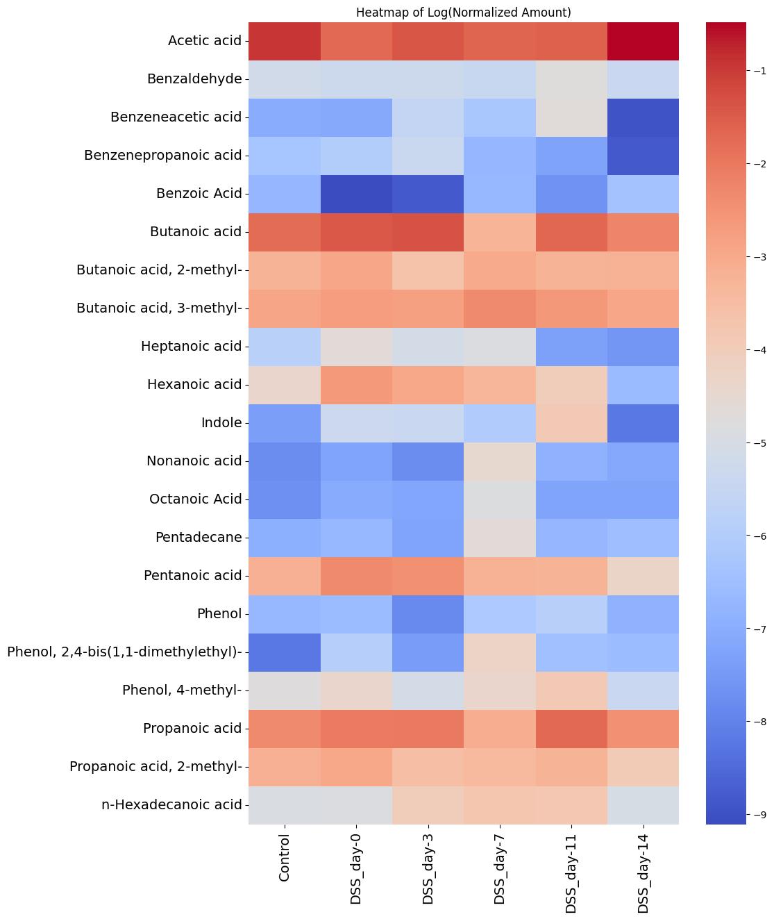
Figure 12. Heatmap of stable metabolites (log transformation) identified in the sodium dextran sulfate (DSS) and control groups over time
2. Initially, a comparison was made between the experimental group of animals receiving DSS and the control group on day 0. The Mann–Whitney statistical test with Bonferroni correction for multiple comparisons was used. No statistically significant differences were identified. The results for 10 stable metabolites detected are shown in Figure 13.
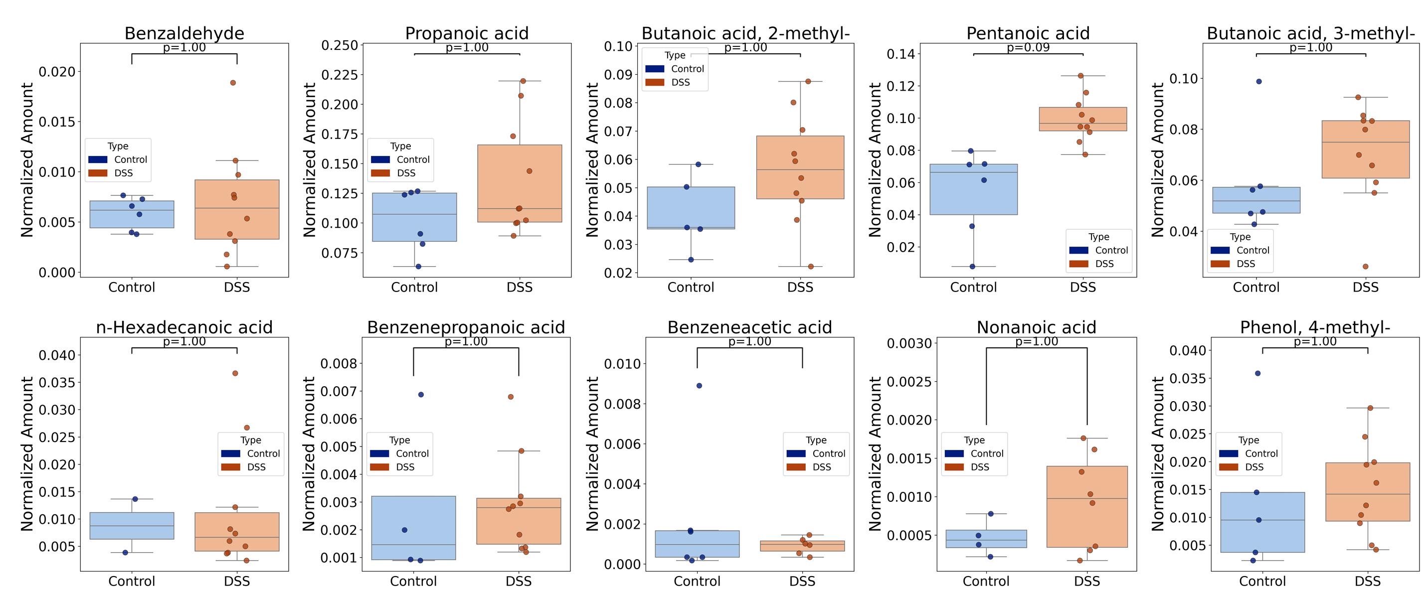
Figure 13. Boxplots comparing the concentrations of 10 stable, detected metabolites in the experimental and control groups on day 0 evaluated by Mann–Whitney tests with Bonferroni correction for multiple comparisons
3. Furthermore, a series of pairwise Mann–Whitney statistical tests with Bonferroni correction for multiple comparisons was conducted to compare the groups of animals that participated in the experiment for 7 and 14 days (DSS7 and DSS14). The comparison was conducted exclusively on the basis of stable detected metabolites. No statistically significant differences were identified. Therefore, the stratification of the experimental groups into two categories (DSS7 and DSS14) had no impact on the subsequent outcomes. The comparison of metabolomic profile data for the four most stable detected compounds between the two groups and across different days of the experiment is presented in Figure 14.
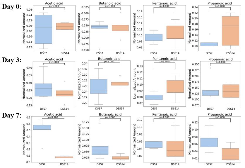
Figure 14. Boxplots comparing the concentrations of the four most stable detected metabolites between the two groups and across different days of the experiment evaluated by Mann–Whitney tests with Bonferroni correction for multiple comparisons
4. Figure 15 illustrates the clear separation of the groups through the use of PCA and orthogonal projections to latent structures discriminant analysis (OPLS-DA) clustering, as well as the average concentrations of consistently detected metabolites across different groups in a heatmap.
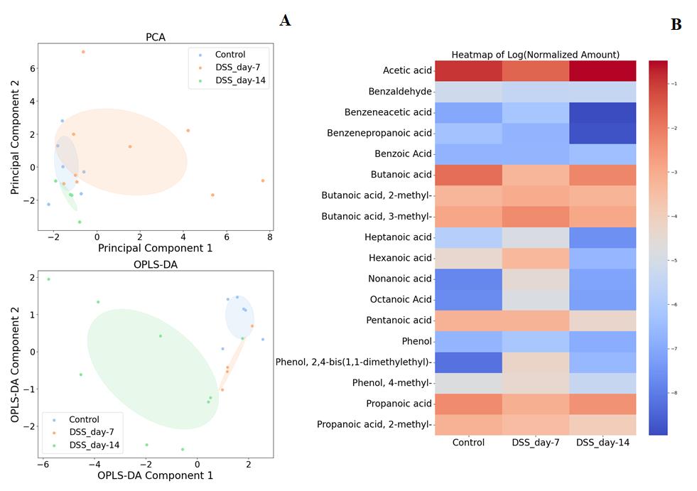
Figure 15. Comparison of the metabolomic profile data of sodium dextran sulfate (DSS) group rats on days 7 and 14 with the control group. A. PCA, OPLS-DA. B. Heatmap.
5. The changes in the average concentration of six consistently detected metabolites from day 7 to the recovery on day 14 in the DSS and control groups are shown in Figure 16.
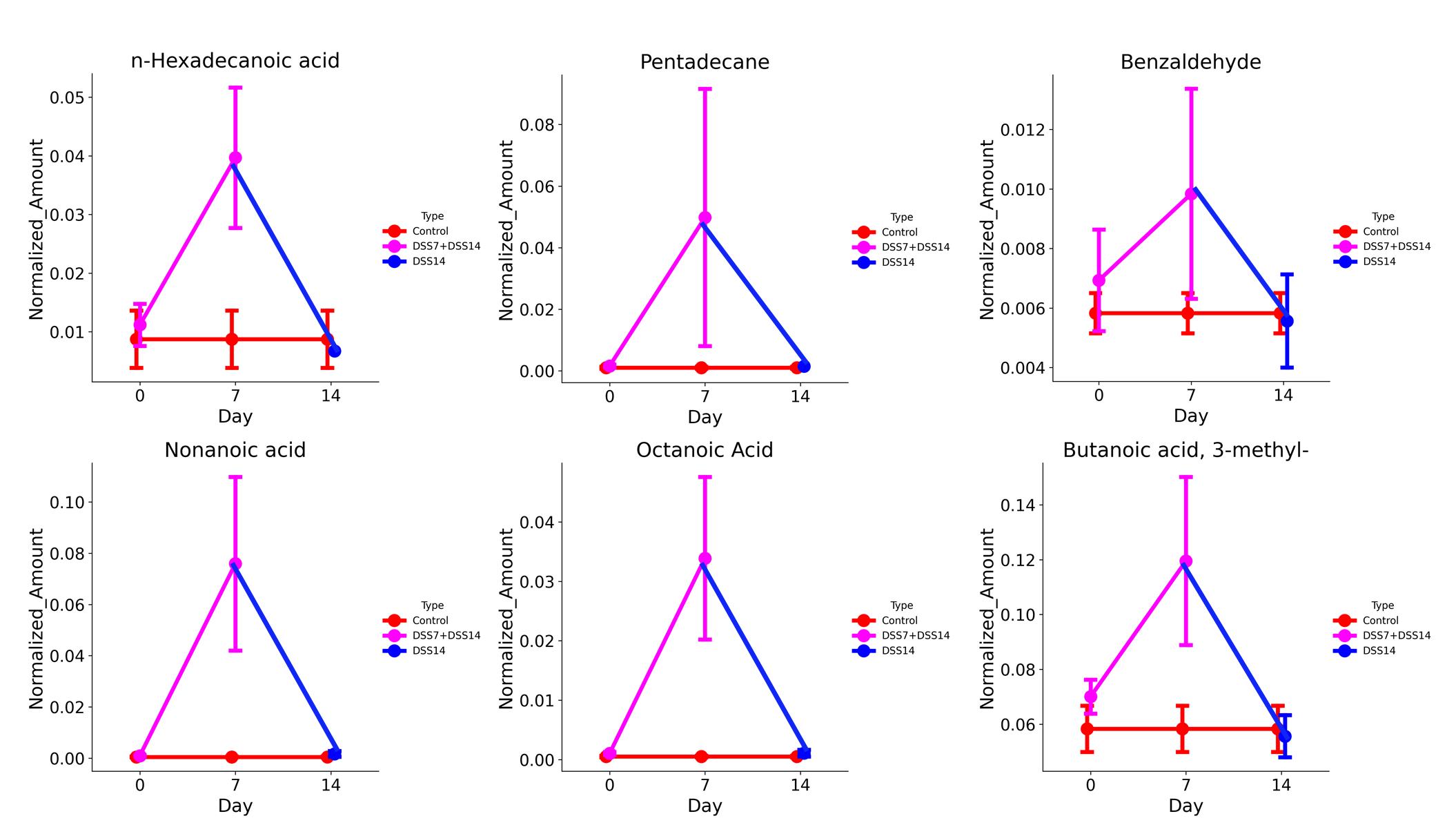
Figure 16. Changes in the average concentration of six consistently detected metabolites in the sodium dextran sulfate (DSS) group compared to the control group
Validation of protocol
This protocol or parts of it has been used and validated in the following research articles:
• Shagaleeva et al. [19]. GC–MS with Headspace Extraction for Non-Invasive Diagnostics of IBD Dynamics in a Model of DSS-Induced Colitis in Rats. International Journal of Molecular Sciences (Figures 1–3, Table 1).
• Shagaleeva et al. [9]. Investigating volatile compounds in the Bacteroides secretome. Frontiers in microbiology (HS-GC/MS study of the volatile spectrum of Bacteroides secretome – Figures 3, 4; HS-GC/MS analysis of outer membrane vesicles (OMVs) – Figures 5, 6)
• Shagaleeva et al. [20]. Therapeutic Effects of Bacteroides fragilis Vesicles in a Model of Chemically Induced Colitis in Rats. Bulletin of Experimental Biology and Medicine (Figures 2, 3 – histology and DAI).
• Shagaleeva et al. [21]. Bacteroides vesicles promote functional alterations in the gut microbiota composition. Microbiology Spectrum (Figure 1 – histology and DAI for DSS-induced colitis mice model; Figures 2, 3 and Table 1 – HS-GC/MS analysis of stool for DSS-induced colitis mice model)
Acknowledgments
This research was supported by RSF grant 24-75-10100. This protocol was based on Int J Mol Sci (2024), DOI: 10.3390/ijms25063295 [19].
Competing interests
The authors declare that the research was conducted in the absence of any commercial or financial relationships that could be construed as a potential conflict of interest.
Ethical considerations
The animal study protocol was approved by the local ethics committee of V.P. Serbsky National Medical Research Center for Psychiatry and Narcology (Protocol No. 8, dated 13 February 2019).
References
- Adamkova, P., Hradicka, P., Kupcova Skalnikova, H., Cizkova, V., Vodicka, P., Farkasova Iannaccone, S., Kassayova, M., Gancarcikova, S. and Demeckova, V. (2022). Dextran Sulphate Sodium Acute Colitis Rat Model: A Suitable Tool for Advancing Our Understanding of Immune and Microbial Mechanisms in the Pathogenesis of Inflammatory Bowel Disease. Vet Sci. 9(5): 238. https://doi.org/10.3390/vetsci9050238
- Mezoff, E. A., Williams, K. C. and Erdman, S. H. (2020). Gastrointestinal Endoscopy in the Neonate. Clin Perinatol. 47(2): 413–422. https://doi.org/10.1016/j.clp.2020.02.012
- Valdés, L., Cuervo, A., Salazar, N., Ruas-Madiedo, P., Gueimonde, M. and González, S. (2015). The relationship between phenolic compounds from diet and microbiota: impact on human health. Food Funct. 6(8): 2424–2439. https://doi.org/10.1039/c5fo00322a
- Wang, B., Yao, M., Lv, L., Ling, Z. and Li, L. (2017). The Human Microbiota in Health and Disease. Engineering. 3(1): 71–82. https://doi.org/10.1016/J.ENG.2017.01.008
- Niccolai, E., Baldi, S., Ricci, F., Russo, E., Nannini, G., Menicatti, M., Poli, G., Taddei, A., Bartolucci, G., Calabrò, A. S., et al. (2019). Evaluation and comparison of short chain fatty acids composition in gut diseases. World J Gastroenterol. 25(36): 5543–5558. https://doi.org/10.3748/wjg.v25.i36.5543
- Zhang, V. R., Ramachandran, G. K., Loo, E. X. L., Soh, A. Y. S., Yong, W. P. and Siah, K. T. H. (2023). Volatile organic compounds as potential biomarkers of irritable bowel syndrome: A systematic review. Neurogastroenterol Motil. 35(7): e14536. https://doi.org/10.1111/nmo.14536
- Liu, S., Zhao, W., Lan, P. and Mou, X. (2020). The microbiome in inflammatory bowel diseases: from pathogenesis to therapy. Protein Cell. 12(5): 331–345. https://doi.org/10.1007/s13238-020-00745-3
- Filipiak, W., Żuchowska, K., Marszałek, M., Depka, D., Bogiel, T., Warmuzińska, N. and Bojko, B. (2022). GC-MS profiling of volatile metabolites produced by Klebsiella pneumoniae. Front Mol Biosci. 9: e1019290. https://doi.org/10.3389/fmolb.2022.1019290
- Shagaleeva, O. Y., Kashatnikova, D. A., Kardonsky, D. A., Konanov, D. N., Efimov, B. A., Bagrov, D. V., Evtushenko, E. G., Chaplin, A. V., Silantiev, A. S., Filatova, J. V., et al. (2023). Investigating volatile compounds in the Bacteroides secretome. Front Microbiol. 14: e1164877. https://doi.org/10.3389/fmicb.2023.1164877
- Karu, N., Deng, L., Slae, M., Guo, A. C., Sajed, T., Huynh, H., Wine, E. and Wishart, D. S. (2018). A review on human fecal metabolomics: Methods, applications and the human fecal metabolome database. Anal Chim Acta. 1030: 1–24. https://doi.org/10.1016/j.aca.2018.05.031
- Antoniou, E., Margonis, G. A., Angelou, A., Pikouli, A., Argiri, P., Karavokyros, I., Papalois, A. and Pikoulis, E. (2016). The TNBS-induced colitis animal model: An overview. Ann Med Surg. 11: 9–15. https://doi.org/10.1016/j.amsu.2016.07.019
- Kiesler, P., Fuss, I. J. and Strober, W. (2015). Experimental Models of Inflammatory Bowel Diseases. CMGH Cell Mol Gastroenterol Hepatol. 1(2): 154–170. https://doi.org/10.1016/j.jcmgh.2015.01.006
- Silva, I., Solas, J., Pinto, R. and Mateus, V. (2022). Chronic Experimental Model of TNBS-Induced Colitis to Study Inflammatory Bowel Disease. Int J Mol Sci. 23(9): 4739. https://doi.org/10.3390/ijms23094739
- Weigmann, B. and Neurath, M. F. (2016). Oxazolone-Induced Colitis as a Model of Th2 Immune Responses in the Intestinal Mucosa. Methods Mol Biol. 1422: 253–261. https://doi.org/10.1007/978-1-4939-3603-8_23
- Martin, J. C., Bériou, G. and Josien, R. (2016). Dextran Sulfate Sodium (DSS)-Induced Acute Colitis in the Rat. Methods Mol Biol. 1371: 197–203. https://doi.org/10.1007/978-1-4939-3139-2_12
- Johansson, M. E. V., Gustafsson, J. K., Holmén-Larsson, J., Jabbar, K. S., Xia, L., Xu, H., Ghishan, F. K., Carvalho, F. A., Gewirtz, A. T., Sjövall, H., et al. (2014). Bacteria penetrate the normally impenetrable inner colon mucus layer in both murine colitis models and patients with ulcerative colitis. Gut. 63(2): 281–291. https://doi.org/10.1136/gutjnl-2012-303207
- Xu, H. M., Huang, H. L., Liu, Y. D., Zhu, J. Q., Zhou, Y. L., Chen, H. T., Xu, J., Zhao, H. L., Guo, X., Shi, W., et al. (2021). Selection strategy of dextran sulfate sodium-induced acute or chronic colitis mouse models based on gut microbial profile. BMC Microbiol. 21(1): 1–14. https://doi.org/10.1186/s12866-021-02342-8
- Wang, J. L., Han, X., Li, J. X., Shi, R., Liu, L. L., Wang, K., Liao, Y. T., Jiang, H., Zhang, Y., Hu, J. C., et al. (2022). Differential analysis of intestinal microbiota and metabolites in mice with dextran sulfate sodium-induced colitis. World J Gastroenterol. 28(43): 6109–6130. https://doi.org/10.3748/wjg.v28.i43.6109
- Shagaleeva, O. Y., Kashatnikova, D. A., Kardonsky, D. A., Danilova, E. Y., Ivanov, V. A., Evsiev, S. S., Zubkov, E. A., Abramova, O. V., Zorkina, Y. A., Morozova, A. Y., et al. (2024). GC-MS with Headspace Extraction for Non-Invasive Diagnostics of IBD Dynamics in a Model of DSS-Induced Colitis in Rats. Int J Mol Sci. 25(6): 3295. https://doi.org/10.3390/ijms25063295
- Shagaleeva, O. Y., Kashatnikova, D. A., Vorobyeva, E. A., Kardonsky, D. A., Silantiev, A. S., Efimov, B. A., Ivanov, V. A., Bespyatikh, Y. A. and Zakharzhevskaya, N. B. (2024). Therapeutic Effects of Bacteroides fragilis Vesicles in a Model of Chemically Induced Colitis in Rats. Bull Exp Biol Med. 177(5): 626–629. https://doi.org/10.1007/s10517-024-06237-2
- Shagaleeva, O. Y., Kashatnikova, D. A., Kardonsky, D. A., Efimov, B. A., Ivanov, V. A., Smirnova, S. V., Evsiev, S. S., Zubkov, E. A., Abramova, O. V., Zorkina, Y. A., et al. (2024). Bacteroides vesicles promote functional alterations in the gut microbiota composition. Microbiol Spectrum. 12(11): e00636–24. https://doi.org/10.1128/spectrum.00636-24
Article Information
Publication history
Received: Dec 4, 2024
Accepted: Feb 7, 2025
Available online: Mar 5, 2025
Published: Mar 20, 2025
Copyright
© 2025 The Author(s); This is an open access article under the CC BY-NC license (https://creativecommons.org/licenses/by-nc/4.0/).
How to cite
Shagaleeva, O. Yu., Kashatnikova, D. A., Kardonsky, D. A., Efimov, B. A., Ivanov, V. A., Smirnova, S. V., Zorkina, Y. A., Vorobjeva, E. A., Silantiev, A. S., Kazakova, V. D., Kolesnikova, I. V., Markelova, M. I., Vanyushkina, A. A., Chaplin, A. V., Grigoryeva, T. V. and Zakharzhevskaya, N. B. (2025). HS–GC–MS Method for the Diagnosis of IBD Dynamics in a Model of DSS-Induced Colitis. Bio-protocol 15(6): e5246. DOI: 10.21769/BioProtoc.5246.
Category
Microbiology > Microbe-host interactions > Bacterium
Biological Sciences > Biological techniques > Mass spectrometry
Medicine > Inflammation
Do you have any questions about this protocol?
Post your question to gather feedback from the community. We will also invite the authors of this article to respond.