- Protocols

- Articles and Issues
- For Authors
- About
- Become a Reviewer

Computational Cellular Mathematical Model Aids Understanding the cGAS-STING in NSCLC Pathogenicity
(*contributed equally to this work) Published: Vol 15, Iss 5, Mar 5, 2025 DOI: 10.21769/BioProtoc.5223 Views: 2913
Reviewed by: Ran ChenXiaokang WuRobert Kiewisz
Original research article
The authors used this protocol in:
Dec 2024
Advertisement


Protocol Collections
Comprehensive collections of detailed, peer-reviewed protocols focusing on specific topics


Related protocols
Abstract
Non-small cell lung cancer (NSCLC) is the most common type of lung cancer. According to 2020 reports, globally, 2.2 million cases are reported every year, with the mortality number being as high as 1.8 million patients. To study NSCLC, systems biology offers mathematical modeling as a tool to understand complex pathways and provide insights into the identification of biomarkers and potential therapeutic targets, which aids precision therapy. Mathematical modeling, specifically ordinary differential equations (ODEs), is used to better understand the dynamics of cancer growth and immunological interactions in the tumor microenvironment. This study highlighted the dual role of the cyclic GMP-AMP synthase–stimulator of interferon genes (cGAS/STING) pathway's classical involvement in regulating type 1 interferon (IFN I) and pro-inflammatory responses to promote tumor regression through senescence and apoptosis. Alternative signaling was induced by nuclear factor kappa B (NF-κB), mutated tumor protein p53 (p53), and programmed death-ligand1 (PD-L1), which lead to tumor growth. We identified key regulators in cancer progression by simulating the model and validating it with the following model estimation parameters: local sensitivity analysis, principal component analysis, rate of flow of metabolites, and model reduction. Integration of multiple signaling axes revealed that cGAS-STING, phosphoinositide 3-kinases (PI3K), and Ak strain transforming (AKT) may be potential targets that can be validated for cancer therapy.
Key features
• Procedures for the reconstruction of a robust and steady-state mathematical model with respective analysis in order to provide mechanistic insights.
• The dynamic mathematical model allows an understanding of the multifaceted dual roles of cGAS-STING in NSCLC promotion and inhibition.
• The inherent statistical tool in systems biology provides a novel immunotherapeutic target.
Keywords: MATLABGraphical overview
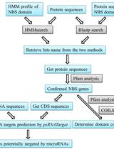
Flowchart of system-based mathematical modeling for the reconstruction of signaling network
Background
Lung cancer is the leading cause of cancer-related deaths worldwide, accounting for approximately 1.79 million fatalities annually [1]. Non-small cell lung cancer (NSCLC) accounts for 85% of cases, with low survival rates with existing treatments. In recent years, NSCLC therapy has undergone an enormous shift since the identification of immunological checkpoints and the subsequent development of immune checkpoint inhibitors (ICIs) [2]. Immunocheckpoint blockade (ICB) targeting the programmed cell death-1/programmed death-ligand1 (PD-1/PD-L1) pathway has become a new standard treatment for NSCLC, improving survival rates either when used alone or in conjunction with conventional chemotherapy [3]. Despite recent developments in immunotherapy, more research is still required to fully comprehend the biology of immune-responsive subsets.
The immune system may be stimulated, and the tumor response to immunotherapy may be improved, by DNA damage, which can be intrinsic due to tumor genomic instability or exacerbated as a result of DNA-damaging treatments [4]. The cGAS-STING signaling pathway is a crucial cytosolic DNA sensing mechanism in vivo, involved in inducing the expression of type I interferons (IFNs) and influencing the body's immune response in controlling pathogen infection, tumor immunity, and autoimmune disorders. cGAS contains an extremely conserved nucleotidyltransferase domain that may detect double-stranded DNA (dsDNA) released into the cytosol [5]. This cGAS-STING signaling in turn triggers IFN I and cytokine response [6–8]. Since aberrant DNA is particularly prominent in cancer as a result of its release from necrotic cells and DNA leakage into the cytosol of cancer cells [9], cGAS signaling may trigger IFN I synthesis, immunological activation, and cancer cell apoptosis. Consequently, downregulating the cGAS-STING pathway would make it possible for cancer cells to avoid immune recognition and response. Furthermore, this pathway's activation can upregulate PD-L1, inhibiting cytotoxic T lymphocyte (CTLs) activity [10]; mutant p53 has also been shown to suppress downstream signaling from cGAS/STING pathway, thereby enabling immune evasion [11].
We studied the cGAS-STING pathway using systems biology, a holistic approach to decode complex, dynamic biological systems with numerous interrelationships and interactions that occur within the confines of time, physiology, and space [12–14]. One crucial tool in systems biology is mathematical modeling, which determines how biological system components interact to produce intricate dynamic behavior. Computational experiments using mathematical models to simulate biological systems could provide valuable insights into the driven mechanisms [15,16]. A unique systems biology toolbox is offered within the MATLAB framework, providing researchers with a versatile platform to explore biological systems, design algorithms, and create simulation tools [17–19]. In this study, we used mathematical modeling to address a knowledge gap by reconstructing the cGAS-STING signaling pathway using MATLAB and understanding its regulatory and molecular drivers through iterative model simulations and data analysis. This included the identification and validation of statistical parameters of the model, such as sensitivity, principal components, and model reduction. Altogether, these studies present a mathematical model as a framework to redesign complex signaling networks; modulating such signaling axes could allow better therapeutic intervention.
Equipment
1. HP Pro 3090MT
Software and datasets
1. MATLAB v7.11.1.866's (SimBiology tool box) (https://www.mathworks.com/products/simbiology.html)
2. COPASI 4.22 (https://copasi.org/)
3. Sigmaplot 10.0 (https://sigmaplot.en.softonic.com/)
4. Microsoft Excel (https://www.microsoft.com/en-us/microsoft-365/previous-versions/microsoft-office-2013)
Procedure
A. Reconstruction of the mathematical model
Obtaining valuable insights into the dynamic behavior of biological systems can be achieved by conducting computational experiments that simulate these systems using mathematical models [15]. The Functional Mock-up Interface (FMI) outlines an interface and a container for exchanging dynamic simulation models [20]. Currently, MATLAB and the SimBiology tool are the only tools used in systems biology that also support FMI [21]. MATLAB v7.11.1.866's SimBiology toolbox was used for the reconstruction of the mathematical model. Designed for pharmacokinetic/pharmacodynamics (PK/PD) and system biology applications, SimBiology is a programmed tool for modeling, simulating, and analyzing dynamic systems. Models can be built programmatically with the MATLAB® language or with the help of a block diagram editor, which supports systems biology markup language (SBML) format [22].
1. Launch MATLAB R2010 and, in the command line, execute the command >SIMBIOLOGY to open the SimBiology toolbox.
2. In the workspace present in the diagram editor, choose the Compartment option from Block Model Browser-model building tab and drop it on canvas. Rename the compartment as “Plasma membrane” (PM).
3. Repeat step A2 by dragging and dropping the compartment on canvas to replicate cellular compartments, which includes plasma membrane, cytoplasm (C), nucleus (Nu), endoplasmic reticulum (ER), and Golgi.
4. Drag and drop Species in the compartment and rename them according to the cellular component, which includes signaling intermediates, receptors, agonists, and transcription factors.
5. Define the reactions by connecting the species through directed edges by dragging and dropping the Reactions from the Model building tab.
6. Connect the substrate species to the reaction by pressing CTRL, then click on Substrate and reaction. Connect the product by pressing CTRL, then click on Reaction and product. This makes the nodes of the signaling network link through directed edges in the form of reactions, which can be parametrized by mathematical and kinetic rate laws and discrete parameters.
7. Define the rate laws and parameters for every reaction by clicking on Reaction; then change the reaction properties and the settings. Define the reactions that follow association, dissociation, and translocation kinetics using the law of mass action (LMA). In the presented model, these were defined for receptor-agonist interactions, dimerization, translocation, and complex formation reactions. Refine the reactions’ initial concentration [S] and rate of reaction (k).
8. Define reactions involving enzyme kinetics such as phosphorylation, dephosphorylation, ubiquitination, acetylation, and methylation using Michaelis–Menten (MM) kinetics. Follow Step A7 to refine these reactions by modifying Maximum velocity (Vmax), Michaelis constant (Km), and [S].
9. Define gene expression reactions that are prominent in the nucleus using Hill’s kinetics. Follow step A7 to refine Vmax, Hill coefficient (n), Km, and [S]. Signaling is induced when receptors dimerize and agonists bind to receptors. In this reaction, receptors and agonists act as the substrate for the formation of the signaling initiator complex, which is the product. This product is a resulting component, which is made of a receptor and an agonist assembly (Figure 1A). When the product from the previous reaction is utilized in the next reaction for the formation of a secondary signaling molecule, then the receptor–agonist complex acts as the substrate and is subsequently utilized in the next reaction step for the formation of the secondary signaling molecule, which acts as a product (Figure 1B).
10. Define all the reactions and discretely refine the model through initial concentration, Vmax, n, and Km. Set the Initial concentrations of the species in the range of 103–106 signaling molecules [23]. Set the initial amount of substrate by adding the number of Molecules as the value unit.
B. Building and simulating cGAS-STING regulation model in NSCLC
To reconstruct the inter-regulatory model, one of the underlying kinetic laws is the law of mass action. The representation of the components involves the law of mass action: [Plasma membrane].Interleukin 10 Receptor (IL10R) + [Plasma membrane].Interleukin 10 (IL10) -> Cytoplasm.Interleukin 10 and Interleukin 10 receptor complex [IL10-R complex] (Figure 1C).
1. Define the LMA reaction as (Forward Rate Parameter)*(MassAction Species) and set the parameters for rate constant for the forward reaction (kf) by defining the value, scope, and value units as per the degree of freedom of reaction. Feed in the initial concentrations of components in the substrate option and use molecules as the unit.
Reactions with enzyme kinetics such as phosphorylation and dephosphorylation reactions are one of the prominent edges between interconnected nodes. Representation of the reaction is [Cytoplasm].Interleukin-1 receptor-associated kinase 4 (IRAK4) -> [Cytoplasm].Interleukin-1 receptor-associated kinase 1 (IRAK1) (Figure 1D).
2. Define the Henri–Michaelis–Menten with reactions in the Reaction properties toolbox with the expression as Vm*S/(Km + S). Set the value and units for Vm and Km to molecule/second and molecules, respectively, and set the initial concentration unit to molecules. Gene transcription involving transcription factors uses Hill’s kinetics. These reactions are prominent for the expression of cytokines in the network. Representation of the reaction is [Nucleus].NFκB -> [Nucleus].PD-L1 (Figure 1E).
3. Expression of the reaction is Vm*S^n/(Kp + S^n) equilibrium constant of Hills kinetics (Kp). Define the scope and values of Vm, n, and Kp as molecules/second, dimensionless, and molecules, respectively.
4. To analyze the effect of mutated p53 on STING-Tank binding kinase 1 (STING-TBK1) complex, use a competitive inhibition reaction. It is defined as C.[Mutated P53] -> C.[Inhibitory STING-TBK1 complex] + C.[Mutated P53] (Figure 1F). Boundary conditions define the system domain bound in a particular state. This condition is fundamental to components that do not show mechanical displacement from cellular compartments.
5. Apply Boundary conditions to components present in plasma membrane, which includes the receptor and their agonist. Also, apply it to the genomic DNA of the cell as it is localized discreetly in the nucleus [24]. Simulation graphs of these reactions are represented in Figure 1C–F.
Figure 1. Simulation graph of rate laws and kinetics. A. Initiation signaling through the law of mass action. B. Secondary signaling followed through the initiator complex. C. Law of mass action. D. Michaelis-Menten kinetics. E. Hill’s kinetics. F. Inhibitory reaction.
C. Simulation of the mathematical model
Assessment of the model behavior is used to understand the alteration in the system's mathematical representation as a result of parameters and kinetics using ODEs. These give an estimate of concentration vs. time for species present in the model. These define the state or phenotype of the model, providing discretization to the model with experimental knowledge.
1. To perform simulation, in the tool bar, click on Tasks, select Add tasks to the model, and then choose Simulate model (Figure 2A–H) (step A1–6).
2. In Configuration settings, choose Data logging option and click on Select all species (Figure 2I).
3. In Simulation settings and Solver type, choose ODE15s (stiff/NDF) solver (Figure 2J).
For all reactions, run a deterministic simulation using the ODE15s (stiff/NDF) solver. Using variable-order numerical differentiation formulas (NDFs), the solver determines the model's state at the next time step.
4. Set up the simulation parameters as mentioned and keep absolute and relative tolerance settings as defaults. Set the time to 100 unit time (s) (Figure 2J), simulate the model by pressing CTRL+T, and observe the simulation graph (Figure 2K).
Figure 2. Representative steps for the reconstruction of a mathematical model using SimBiology toolbox. A. Launch MATLAB R2010b. B. In the Command window, type “SIMBIOLOGY” or “symbiology” to launch the SimBiology toolbox. C. Click on Diagram view to visualize the canvas. D–E. From the Block Library Browser, drag and drop the compartment and label it accordingly. F. Drag and drop species and reaction in the compartment. G. Press CTRL and connect species 1 (PI3K for representation) with the reaction. Repeat the step with species 2 (AKT). Double-click on the reaction and set the parameters, which mainly include kinetic law, kinetic law parameter, value, units, and substrate concentration. Make sure that the Active reactive check box is ticked. H. In Tasks, select Add model task to the untitled and select Simulate model. I. In the Configuration settings and data logging option, select and tick the species in the checkbox of log column. J. In the Settings option adjacent to data logging, select the solver type as ode15s (stiff/NDF) and change the stop time to 100.0 simulation time (seconds). K. Press CTRL+T and observe the concentration vs. time plot for the reaction.
D. Sensitivity analysis
Sensitivity analysis assesses the robustness of the mathematical model. Sensitivity analysis is a technique that involves altering the parameters of each reaction in the system to increase the mathematical model's robustness. With regard to the initial concentration of the species and the model's rate laws and kinetics defining parameter values, local sensitivity computes the time-dependent sensitivities of each species state. The time-dependent sensitivities of x with respect to each parameter value can therefore be represented at the time-dependent derivatives as Eq. dx/dy, dx/dz, where the numerators are the sensitivity outputs and the denominators are the sensitivity inputs to sensitivity analysis. This is applicable to models with species x and two parameters, y and z.
1. For obtaining sensitivity coefficients, deselect all the species from data logging. Furthermore, in the model task panel, add sensitivity as a task (Figure 3A and 3B).
2. In Settings option, choose the solver type as SUite of Nonlinear and DIfferential/ALgebraic equation Solvers (SUNDIALS). Set the Absolute tolerance to 1.0 × 10⁻⁶ and relative tolerance to 0.0010 (Figure 3C).
3. In Sensitivity settings, in Mode of sensitivity, choose None for normalization. Add each species name to the Component name table. Calculate the sensitivity coefficient for each species by keeping only one component as input and all others as output (Figure 3D).
4. Press CTRL+T and the graph will display the sensitivity coefficients of the components that are sensitive toward the input species. Using the Data cursor in the Plot browser, note the sensitivity coefficients for species when they reach the steady state (Figure 3E).
Figure 3. Representative steps for sensitivity analysis of the mathematical model in the SimBiology toolbox. A. In Configuration settings and data logging window, deselect all species by unchecking the Log column tick box. B. In the Task tab, select Add model task to untitled and select Calculate sensitivities. C. In the Sensitivities model task, click on Settings and change the Solver type to Sundials. D. In Sensitivity settings, choose None for normalization. Add the species name in the output and input tables. Select one component as input and keep all others as output. E. Press CTRL+T and observe the sensitivity coefficient graph. Construct the adjacency matrix in Microsoft Excel as demonstrated in Figure 6.
E. Principal component analysis (PCA)
The purpose of PCA is to reduce dimensionality and eliminate background noise from biological data. Each system component's varying sensitivity is represented by its principal component (PC) score. A high PC score indicates that a component in the system is highly sensitive; if that component is to be targeted, the system could potentially collapse. Network biology defines highly linked nodes as those that have the propensity to transmit the greatest amount of biological information from one end to the other. The biological information flow that is disrupted in this context and consequently has a significant influence on the system's output is referred to as collapse.
1. As the total number of species in the model is 69, construct a diagonal adjacency matrix of (m*n), which will be (69*69) in the Excel workbook.
2. In the MATLAB command line, write the command as a = [m*n]. This command will generate a score-efficient table, which will be later used to identify PCs.
3. Then, write the command [score_coefficient] = princomp(a). A table is generated with a PCA score coefficient of all components.
F. Flux analysis
Every reaction's productivity is determined by its flow, which also determines each reaction's contribution to the system through flux.
1. For flux analysis, export the model in SBML format and analyze it on COPASI.4.22. by importing the SBML file.
2. In the Steady state option, set the parameters as follows to obtain the flux for each reaction: Jacobian and stability settings should be On, Set resolution to 1 × 10⁻⁹, Derivation factor to 0.001, keep Newton and integration for steady state analysis on, set iteration limit to 50, set maximum duration for forward integration to 1,000,000,000, set maximum duration for backward integration to 1,000,000, and set target criterion to distance and rate.
3. High flux reactions will be displayed in the Reaction tab in the Results section of steady state.
G. Model reduction
By removing reactions that have little to no effect on the system's overall dynamics, this method is used to simplify the system. Removing redundant and spurious parameters of transient reaction intermediates that do not add utility to the system streamlines the mathematical model and makes it easier to anticipate the biological system with accuracy without exhibiting any transient behavior.
1. Note the essential components controlling the system dynamics using species concentration, flux, and sensitivity analysis. Construct the model reduction by adding sensitivity coefficients, concentration, and flux of each species in an Excel workbook table.
2. Analyze the matrix using Sigmaplot. Input the sensitivity coefficients and flux values from sensitivity analysis and flux analysis.
3. For identification of concentrations, import the model in COPASI and run the time course using the following parameters: set Duration to 100 s, use the Deterministic Linear Solver for Ordinary Differential Equations (LSODA) method, set Relative tolerance to 1 × 10⁻⁶, Absolute Tolerance to 1× 10-12, and Max Internal steps to 100,000.
4. Note the concentration of the components at the time point at which steady-state sensitivity coefficients were identified for a component. Likewise, note the concentration for each species in the matrix.
H. Crosstalk point
Any direct or indirect connection between signaling components of two distinct pathways that affect a biological response is referred to as a crosstalk point. These nodes play a major role in controlling signaling mechanisms and have a tendency to alter the model dynamics in the context of the reconstructed network. The approach assists in identifying the most significant component by examining the network's design; it suggests that the more the crosstalk score, the greater the likelihood that a specific component will promote inflammation.
1. In order to determine the regulatory components of the network, subtract the degree of one particular pathway from the total degree of the network's node.
2. The crosstalk points in the network are signified by the “non-zero value” from the analysis of components in the signaling network.
Data analysis
A. Reconstruction and simulation of the mathematical model
1. The graph of state vs. time will be displayed on the Figure tab.
2. Choose the data cursor option and click on the simulation plot line representing the concentration of the species.
3. To add the name of species to the graph, click on Insert, then click on the Text box, and type the name of the species.
4. The above steps can be repeated for other species in the model. The representation of different types of kinetic graphs is shown in Figure 1A–F. The representation of the reconstructed mathematical (Figure 4) and simulation graph of the top five species with their ODEs is given in Figure 5A and 5B; ODEs of all the components are enlisted in supplementary data (S1).
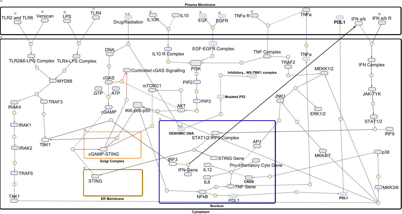
Figure 4. Reconstructed mathematical model of the cGAS-STING pathway in non-small cell lung cancer (NSCLC)
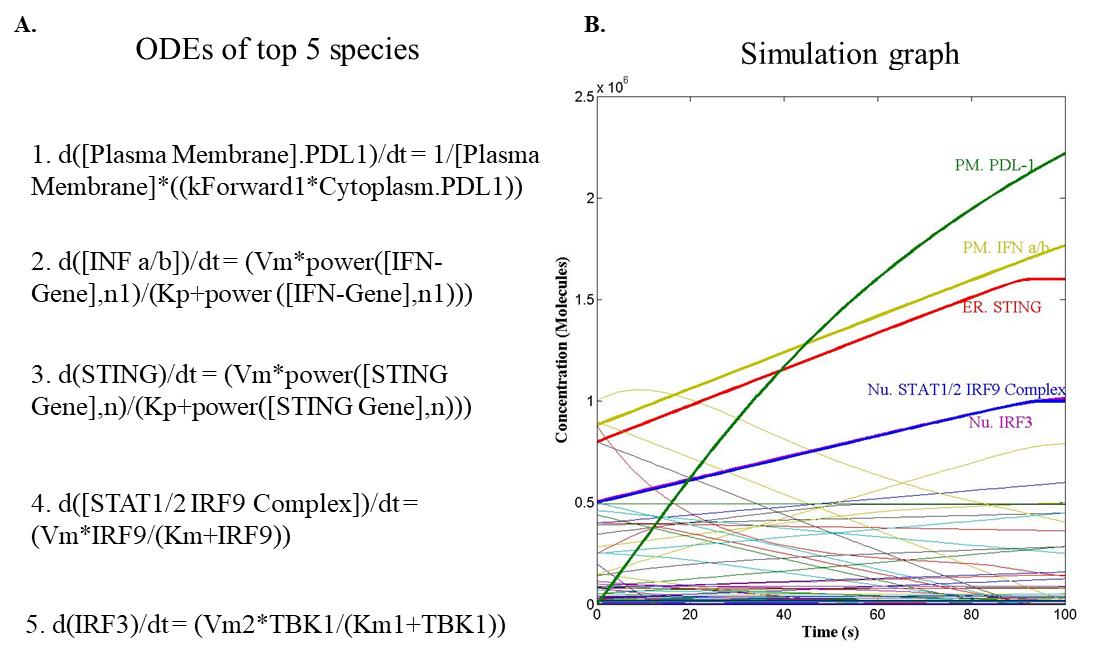
Figure 5. Simulation of the mathematical model at 100 time units. A. Ordinary differential equations (ODEs) of top five components. B. Simulation graph of concentration with respect to time.
B. Model analysis using PCA
1. For the preparation of the PCA plot, launch SigmaPlot. In SigmaPlot, click on File and create a new datasheet.
2. Paste the PCA score efficient table in the sheet. To generate a PCA plot, click on Graph.
3. Select the following options: create graph → scatterplot → multiple scatter → many Y → click finish. Two-dimensional-reduced component graphs will be displayed.
4. To identify the components with PCA scores between 0.8 and 1.0, click on that PCA point to see the representative species number and then refer to the sensitivity matrix for the species’ label.
5. For labeling the PCs, click on Tools and select the Draw arrow option. Then, click on Tools and insert text. For a better understanding of PCA analysis, we demonstrated Toll-like receptor (TLR) signaling with a 4*4 matrix (Figure 6A–C), Representation of the PCA plot is shown in Figure 6D. A sensitivity adjacency matrix and a coefficient table are provided in the supplementary file (S2 and S3).
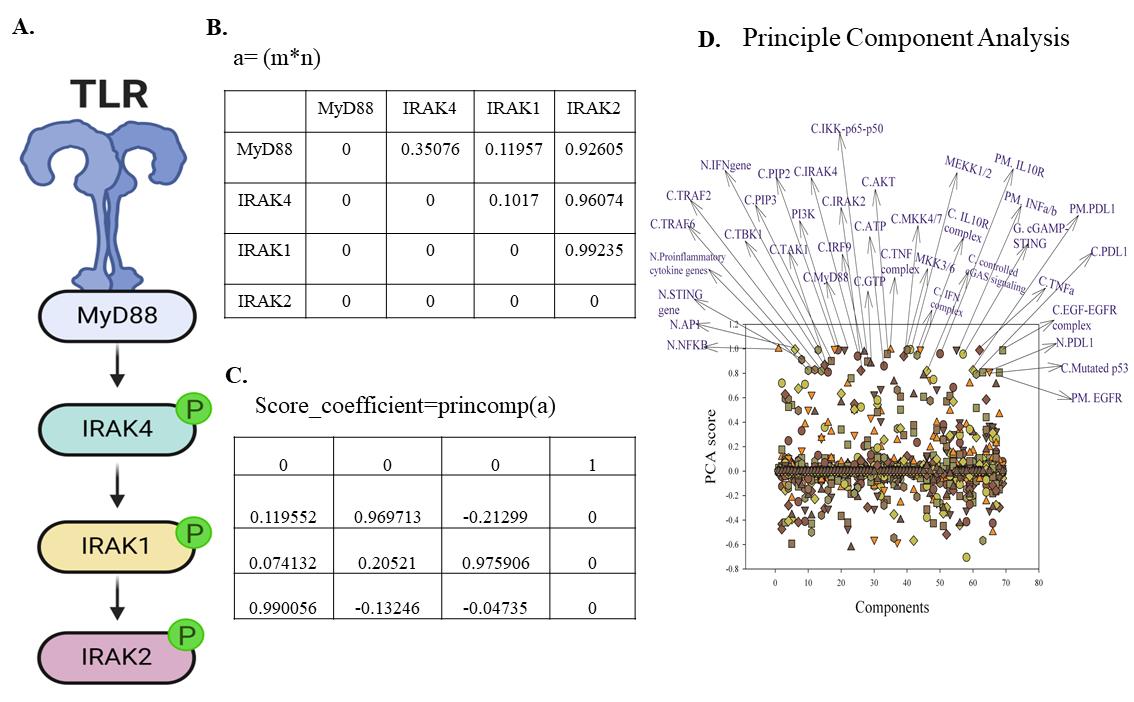
Figure 6. Sensitivity analysis for the identification of principal components of the model. A. Representation of TLR pathway components include myeloid differentiation primary response protein 88 (MyD88), IRAK4, IRAK1, and interleukin-1 receptor-associated kinase 2 (IRAK2). B. 4*4 m*n (matrix) of sensitivity coefficients. C. 4*4 m*n score-coefficient table. D. Principal component analysis.
C. Identifying high flux reactions
Flux analysis identifies components that significantly contribute to the flow of metabolites in the system. The flux of a reaction might be used to understand the dynamics and behavior of the model under various conditions. This analysis can help identify key pathways, steady states, and potential bottlenecks in the system.
1. Import the flux table from COPASI to an Excel sheet.
2. In Home → Editing option, click on Sort and filter. Select largest to smallest.
3. Choose top high flux reactions. Table 1 depicts high flux reactions. Reactions leading to the production of PD-L1, interferon regulatory factor 3 (IRF3), STING, signal transducer and activator of transcription 1 and 2- interferon regulatory factor 9 (STAT1/2 IRF9) complex, and IFN a/b had high flux in the model system. These components were also observed to be highly upregulated in the simulation analysis of the model, suggesting that the model dynamics shifted more toward a cancer proliferation phenotype. The flux of all reactions is listed in the Supplementary Table (S4).
Table 1. High flux reactions of the mathematical model
| Reactions | Flux (molecules/second) |
| PDL1(Nucleus) -> PDL1(Cytoplasm) | 40000 |
| PDL1{Cytoplasm} -> PDL1{"Plasma Membrane"} | 30000 |
| Mitogen-activated protein kinase kinase 3 and 6 (MKK3/6) -> p38 mitogen-activated protein kinases (p38) | 19047.6 |
| NFκB -> PDL1{Nucleus} | 9887.64 |
| IRF3 + IFN-Gene -> "INF a/b" + IRF3 | 8955.22 |
| "STAT1/2 IRF9 Complex" + "STING Gene" -> STING + "STAT1/2 IRF9 Complex" | 8949.66 |
| p38 -> cAMP-response element binding protein (CREB) | 6902.82 |
| STAT1/2+ IRF9 -> "STAT1/2 IRF9 Complex" + STAT1/2 | 5471.82 |
| TBK1 -> IRF3 | 5441.09 |
D. Building quasi-potential landscape for reduced model
1. Export the table in Sigmaplot to generate a three-dimensional quasi-potential landscape. The quasi-potential landscape is a function that is associated with the dynamics of the system with a potential like function, used to represent the stability characteristics of the system.
2. Click Graph → Create graph → Graph type → 3D Mesh Plot → Next. In Data format, choose XYZ triplet.
3. Define X as sensitivity, Y as concentration, and Z as flux.
4. Label the axis by choosing text and labeling the respective axis.
5. To export the image, click on File → Export → Export file. In the pop-up window, click on the drop-down menu for Format. Browse the file location and name it. Click Export. A structural outline of model reduction is shown in Figure 7A. The model was reduced to 83% by filtering out low flux, low concentration, and low sensitivity coefficients defining components. The simplified parameters table is represented in Figure 7B. By further refinement of spurious parameters, reaction intermediates were filtered to obtain a quasi-potential landscape of the reduced model. The dome-shaped graph shows the color scheme from blue to red showing the filtration of significant components in the simplified model. Components with high sensitivity, flux, and time-dependent concentration generated an energy landscape where they positively showed stable states showing local energy minima (Figure 7C). The reaction intermediates showed transition states (saddle points) and unstable states (local maxima). The matrix for model reduction is provided in Supplementary file S5.
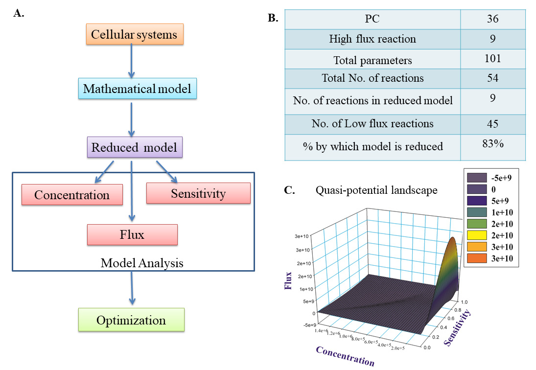
Figure 7. Model reduction of the mathematical model. A. Flowchart for model reduction. B. Simplified parameters after model reduction. C. Quasi-potential landscape.
E. Identifying crosstalk points in the model
1. Open the Excel sheet and list the crosstalk species and non-zero-degree values in columns.
2. Click Insert → Chart → Column → 2D clustered column.
3. For labeling the axis, click Layout → Labels → Axis title.
The term crosstalk was first introduced by Schwartz [25] as a scenario in which two inputs interact to regulate cell development despite acting through different signaling pathways [26]. Modulating such components could provide insights into therapeutic potentials.
The identification of the central node in the network and cellular response was analyzed to identify crosstalk points (Figure 8A, B). Crosstalk points identified from the model were cyclic AMP-GMP nucleotide-STING (cGAMP-STING), inhibitor of nuclear factor-κB (IκB) kinase bound to NFκB subunits (IKK-p65-p50), TBK1, AKT, MyD88, mitogen-activated protein kinase kinase (MEKK), Jun N-terminal kinase (JNK), and PI3K. The non-zero values for the identified components are listed in Figure 8C. Out of all crosstalk points, cGAMP-STING, IKK-p65-p50, AKT, and PI3K had the highest non-zero value (Figure 8C). cGAMP-STING was observed to be a crosstalk between the TLR, cGAS-STING, IL10, and tumor necrosis factor alpha (TNF) signaling pathways. AKT was observed to form a crosstalk between IL10, TNF, and cGAS-STING pathways. PI3K was observed to be a crosstalk between epidermal growth factor receptor (EGFR), IL10, and TNF signaling pathways (Figure 4).
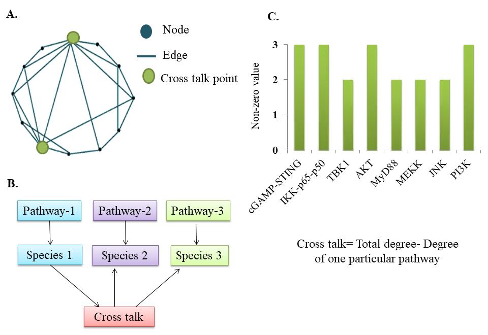
Figure 8. Analysis of crosstalk points. A. Representation of crosstalk points in the network. B. Inter-regulation of pathways converging at crosstalk points. C. Identified crosstalk points.
Validation of protocol
This protocol or parts of it has been used and validated in the following research articles:
• Samarth et al. [27]. Investigation through naphtho[2,3-a]pyrene on mutated EGFR mediated autophagy in NSCLC: Cellular model system unleashing therapeutic potential. IUBMB Life. https://doi.org/10.1002/iub.2914 (Figure 1).
• Gulhane and Singh [28]. MicroRNA-520c-3p impacts sphingolipid metabolism mediating PI3K/AKT signaling in NSCLC: Systems perspective. J. Cell. Biochem. 123(11): 1827–1840. https://doi.org/10.1002/jcb.30319 (Figures 3–8).
General notes and troubleshooting
Capturing all biological interactions and the network-governing complexity of the systems is a challenge when reconstructing mathematical models. Another prominent challenge of systems biology–based mathematical modeling is the development of technologies, especially advanced computers and cutting-edge software, for integration, analysis, and storage of the data. The reconstruction of a mathematical model may provide biological significance when studying a model system, but it is essential that ODEs are mathematically correct after simulation. Concentration vs. time graphs can sometimes show negative values, which are spurious; this demands iterative refinement of simulations. Similarly, sensitivity coefficients must be in the range of 0 to 1 and cannot be negative.
Investigations of cancer immunotherapy using mathematical modeling emphasize clinical translatability. Combining clinical and experimental data allows the reconstruction of complete models for clinical prediction applications and highlights the obstacles that need to be addressed for widespread clinical adaptation to be achieved in various cancer models. The study may highlight potential targets for therapeutic intervention pertaining to the biological question that is often investigated through one or two principal components. As a matter of fact, other important principal components, flux, and cross talks might not be investigated in detail. Nonetheless, those principal components are still crucial for the sustenance of the model's robust behavior.
Supplementary information
The following supporting information can be downloaded here:
1. S1. Ordinary differential equations
2. S2. Sensitivity matrix
3. S3. Score coefficient
4. S4. Flux analysis
5. S5. Model reduction
Acknowledgments
We thank all authors from our corresponding original research paper in the IUBMB Life (2024) [27] and Journal of cellular Biochemistry (2022) [28]. We thank the Department of Biotechnology, Ministry of Science and Technology, Government of India for intramural funding. We also thank the Director, Biotechnology Research and Innovation Council- National Centre for Cell Science (BRIC-NCCS), Pune for supporting the Bioinformatics and High Performance Computing Facility at BRIC-NCCS.
Competing interests
The authors declare no conflicts of interest.
References
- Ferlay, J., Colombet, M., Soerjomataram, I., Parkin, D. M., Piñeros, M., Znaor, A. and Bray, F. (2021). Cancer statistics for the year 2020: An overview. Int J Cancer. 149(4): 778–789. https://doi.org/10.1002/ijc.33588
- Pardoll, D. M. (2012). The blockade of immune checkpoints in cancer immunotherapy. Nat Rev Cancer. 12(4): 252–264. https://doi.org/10.1038/nrc3239
- Ettinger, D. S., Aisner, D. L., Wood, D. E., Akerley, W., Bauman, J., Chang, J. Y., Chirieac, L. R., D'Amico, T. A., Dilling, T. J., Dobelbower, M., et al. (2018). NCCN Guidelines Insights: Non–Small Cell Lung Cancer, Version 5.2018. J Natl Compr Cancer Netw. 16(7): 807–821. https://doi.org/10.6004/jnccn.2018.0062
- Han, D., Zhang, J., Bao, Y., Liu, L., Wang, P. and Qian, D. (2022). Anlotinib enhances the antitumor immunity of radiotherapy by activating cGAS/STING in non-small cell lung cancer. Cell Death Discovery. 8(1): 468. https://doi.org/10.1038/s41420-022-01256-2
- Yang, C., Liang, Y., Liu, N. and Sun, M. (2023). Role of the cGAS-STING pathway in radiotherapy for non-small cell lung cancer. Radiat Oncol. 18(1): 1–7. https://doi.org/10.1186/s13014-023-02335-z
- Sun, L., Wu, J., Du, F., Chen, X. and Chen, Z. J. (2013). Cyclic GMP-AMP Synthase Is a Cytosolic DNA Sensor That Activates the Type I Interferon Pathway. Science. 339(6121): 786–791. https://doi.org/10.1126/science.1232458
- He, L., Xiao, X., Yang, X., Zhang, Z., Wu, L. and Liu, Z. (2017). STING signaling in tumorigenesis and cancer therapy: A friend or foe? Cancer Lett. 402: 203–212. https://doi.org/10.1016/j.canlet.2017.05.026
- Schneider, W. M., Chevillotte, M. D. and Rice, C. M. (2014). Interferon-Stimulated Genes: A Complex Web of Host Defenses. Annu Rev Immunol. 32(1): 513–545. https://doi.org/10.1146/annurev-immunol-032713-120231
- Bakhoum, S. F., Ngo, B., Laughney, A. M., Cavallo, J. A., Murphy, C. J., Ly, P., Shah, P., Sriram, R. K., Watkins, T. B. K., Taunk, N. K., et al. (2018). Chromosomal instability drives metastasis through a cytosolic DNA response. Nature. 553(7689): 467–472. https://doi.org/10.1038/nature25432
- Tian, Z., Zeng, Y., Peng, Y., Liu, J. and Wu, F. (2022). Cancer immunotherapy strategies that target the cGAS-STING pathway. Front Immunol. 13: e996663. https://doi.org/10.3389/fimmu.2022.996663
- Ghosh, M., Saha, S., Li, J., Montrose, D. C. and Martinez, L. A. (2023). p53 engages the cGAS/STING cytosolic DNA sensing pathway for tumor suppression. Mol Cell. 83(2): 266–280.e6. https://doi.org/10.1016/j.molcel.2022.12.023
- Kremling, A. (2013). Systems biology: Mathematical modeling and model analysis. Syst Biol Math Model Model Anal. 3758: 1–362. https://doi.org/10.1080/17513758.2017.1400121
- Mesarović, M. D. (1968). Systems Theory and Biology—View of a Theoretician. Syst Theory Biol. 1141(12): 59–87. https://doi.org/10.1007/978-3-642-88343-9_3
- Kitano, H. (2002). Systems Biology: A Brief Overview. Science. 295(5560): 1662–1664. https://doi.org/10.1126/science.1069492
- Kraikivski, P. (2023). Mathematical Modeling in Systems Biology. Entropy. 25(10): 1380. https://doi.org/10.3390/e25101380
- Voit, E. O. (2022). Perspective: Systems biology beyond biology. Front Syst Biol. 2: e987135. https://doi.org/10.3389/fsysb.2022.987135
- Schmidt, H., Drews, G., Vera, J. and Wolkenhauer, O. (2007). SBML export interface for the systems biology toolbox for MATLAB. Bioinformatics. 23(10): 1297–1298. https://doi.org/10.1093/bioinformatics/btm105
- Schmidt, H. and Jirstrand, M. (2006). Systems Biology Toolbox for MATLAB: a computational platform for research in systems biology. Bioinformatics. 22(4): 514–515. https://doi.org/10.1093/bioinformatics/bti799
- Basak, S., Behar, M. and Hoffmann, A. (2012). Lessons from mathematically modeling the NF‐κB pathway. Immunol Rev. 246(1): 221–238. https://doi.org/10.1111/j.1600-065x.2011.01092.x
- Guilbaud, T., Fiorina, C., Lorenzi, S., Scolaro, A., Carminati, F., Maire, D. and Pautz, A. (2024). Investigating the Functional Mock-up Interface as a Coupling Framework for the multi-fidelity analysis of nuclear reactors. Prog Nucl Energy. 169: 105022. https://doi.org/10.1016/j.pnucene.2023.105022
- Schölzel, C., Blesius, V., Ernst, G., Goesmann, A. and Dominik, A. (2021). Countering reproducibility issues in mathematical models with software engineering techniques: A case study using a one-dimensional mathematical model of the atrioventricular node. PLoS One. 16(7): e0254749. https://doi.org/10.1371/journal.pone.0254749
- Soni, B. and Singh, S. (2021). COVID-19 co-infection mathematical model as guided through signaling structural framework. Comput Struct Biotechnol J. 19: 1672–1683. https://doi.org/10.1016/j.csbj.2021.03.028
- Moran, U., Phillips, R. and Milo, R. (2010). SnapShot: Key Numbers in Biology. Cell. 141(7): 1262–1262.e1. https://doi.org/10.1016/j.cell.2010.06.019
- Xue, C., Friedman, A. and Sen, C. K. (2009). A mathematical model of ischemic cutaneous wounds. Proc Natl Acad Sci USA. 106(39): 16782–16787. https://doi.org/10.1073/pnas.0909115106
- Schwartz, M. A. and Baron, V. (1999). Interactions between mitogenic stimuli, or, a thousand and one connections. Curr Opin Cell Biol. 11(2): 197–202. https://doi.org/10.1016/S0955-0674(99)80026-X
- Klipp, E. and Liebermeister, W. (2006). Mathematical modeling of intracellular signaling pathways. BMC Neurosci. 7: 1–16. https://doi.org/10.1186/1471-2202-7-s1-s10
- Samarth, N., Gulhane, P. and Singh, S. (2024). Investigation through naphtho[2,3‐a]pyrene on mutated EGFR mediated autophagy in NSCLC: Cellular model system unleashing therapeutic potential. IUBMB Life. 76(12): 1325–1341. https://doi.org/10.1002/iub.2914
- Gulhane, P. and Singh, S. (2022). MicroRNA‐520c‐3p impacts sphingolipid metabolism mediating PI3K/AKT signaling in NSCLC: Systems perspective. J Cell Biochem. 123(11): 1827–1840. https://doi.org/10.1002/jcb.30319
Article Information
Publication history
Received: Nov 12, 2024
Accepted: Jan 19, 2025
Available online: Feb 10, 2025
Published: Mar 5, 2025
Copyright
© 2025 The Author(s); This is an open access article under the CC BY-NC license (https://creativecommons.org/licenses/by-nc/4.0/).
How to cite
Khandibharad, S., Gulhane, P. and Singh, S. (2025). Computational Cellular Mathematical Model Aids Understanding the cGAS-STING in NSCLC Pathogenicity. Bio-protocol 15(5): e5223. DOI: 10.21769/BioProtoc.5223.
Category
Bioinformatics and Computational Biology
Systems Biology > Interactome > Gene network
Do you have any questions about this protocol?
Post your question to gather feedback from the community. We will also invite the authors of this article to respond.