- Protocols

- Articles and Issues
- For Authors
- About
- Become a Reviewer

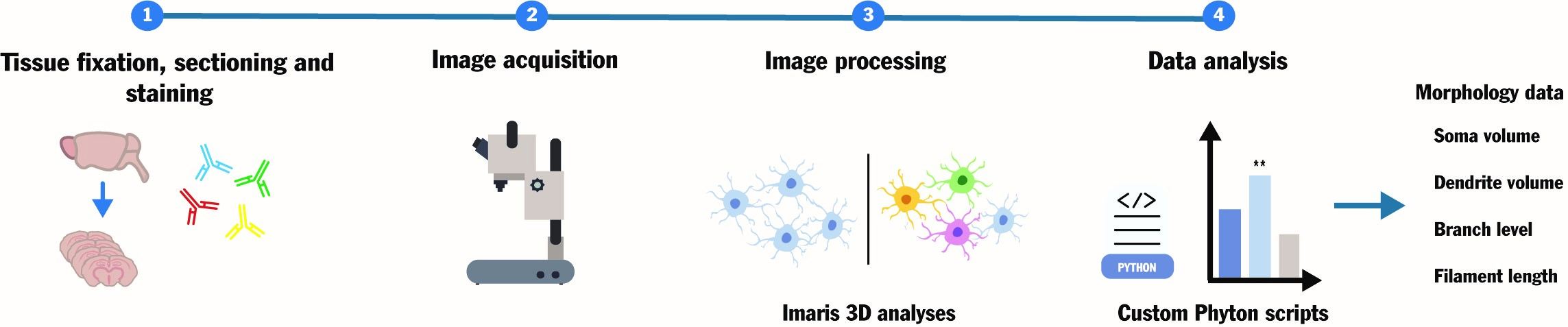
Streamlined Quantification of Microglial Morphology in Mouse Brains Using 3D Immunofluorescence Analysis
Published: Vol 15, Iss 4, Feb 20, 2025 DOI: 10.21769/BioProtoc.5218 Views: 3535
Reviewed by: Olga KopachAnonymous reviewer(s)
Advertisement


Protocol Collections
Comprehensive collections of detailed, peer-reviewed protocols focusing on specific topics


Related protocols

Abstract
Microglial cells are crucial patrolling immune cells in the brain and pivotal contributors to neuroinflammation during pathogenic or degenerative stress. Microglia exhibit a heterogeneous "dendrite-like" dense morphology that is subject to change depending on inflammatory status. Understanding the association between microglial morphology, reactivity, and neuropathology is key to informing treatment design in diverse neurodegenerative conditions from inherited encephalopathies to traumatic brain injuries. However, existing protocols for microglial morphology analyses lack standardization and are too complex and time-consuming for widescale adoption. Here, we describe a customized pipeline to quantitatively assess intricate microglial architecture in three dimensions under various conditions. This user-friendly workflow, comprising standard immunofluorescence staining, built-in functions of standard microscopy image analysis software, and custom Python scripts for data analysis, allows the measurement of important morphological parameters such as soma and dendrite volumes and branching levels for users of all skill levels. Overall, this protocol aims to simplify the quantification of the continuum of microglial pathogenic morphologies in biological and pharmacological studies, toward standardization of microglial morphometrics and improved inter-study comparability.
Key features
• Comparison of 3D microglial architecture between physiological and pathological conditions.
• Quantitative assessment of critical microglial morphological features, including soma volume, dendrite volume, branch level, and filament length.
• Simplified, semi-automated data export and analysis through simple Python scripts.
Keywords: MicrogliaGraphical overview
Background
Neuroinflammation, a main mechanism behind neuronal death and dysfunction in various pathologies, involves microglia as key players patrolling immune cells [1]. These cells, known for their morphological heterogeneity and dynamic processes, play diverse roles in different neurodegenerative disorders [2,3]. It is well-known that the functional and morphological alterations in response to intracellular or extracellular cues are highly interconnected. For example, microglia often exhibit increased volume and altered dendrite architecture when performing phagocytic functions in damaged loci, as opposed to a ramified, homeostatic morphology in healthy brain tissue [4,5].
Given the fundamental role of microglia as resident immune cells in the central nervous system, understanding their behavior in pathological contexts is crucial. In this regard, light microscopy–based immunohistochemical (IHC) analyses of ex vivo brain sections remain a core tool for neuropathology research centers worldwide. However, the dense and intricate microglial architecture poses challenges for 3D morphological studies, necessitating a workflow that builds on standard techniques and tools to facilitate standardization and widespread adoption in neuropathology research. Previous methods for 3D IHC analyses have inherent limitations that result in high error rates when measuring numerous small parameters in large and complex brain samples. This often requires significant time investments, specialized analyses, and multiple software tools. Moreover, commonly used techniques for quantitative microglial assessment lack data standardization, resulting in non-comparable results [5]. This is exemplified by the inherent limitations of common open-source tools, such as ImageJ, which either lack the capability for 3D assessment or require complex pipelines involving non-standardized plug-ins to obtain 3D data [3,6–9].
To overcome these challenges and capture the continuum of microglial morphologies under various physiological and pathological states, we describe a straightforward and repeatable custom approach for 3D microglial morphology analyses in mouse brain sections. Our pipeline is based on 3D image acquisition workflows built into the standard Imaris software, followed by custom Python scripts for data analysis. Similar approaches have been successfully employed for 3D analyses of cell volumes and morphological features, albeit in distinct research fields from neuroscience [10,11]. The protocol described here was used to study neuroinflammation and treatment response in primary mitochondrial disorders, specifically in a mouse model of Leigh syndrome that presents distinct patterns of inflammatory neurodegeneration associated with treatment-resistant epilepsy [12,13].
This workflow may be applicable to multiple conditions, providing biological plausibility for the association between gene disruptions and neuropathological phenotypes. It also enables the assessment of the effects of various pharmacological treatments, thereby informing pre-clinical drug development.
Materials and reagents
Biological materials
1. Mice with conditional Ndusf4 ablation in Gad2-espressing neurons (Gad2Cre/+:Ndufs4lox/lox or Gad2:Ndufs4cKO) were obtained as previously described [12,13]. Gad2Cre/+:Ndufs4lox/+ healthy males, expressing Cre specifically in Gad2-positive cells, were crossed with healthy females that have floxed Ndufs4 exon 2 (Gad2+/+, Ndufs4lox/lox), resulting in Gad2:Ndufs4cKO pups or sex/age-matched controls lacking Cre-expression (Gad2+/+) or functional loxP pair on the target gene (Ndufs4lox/+). A full description of the analyses and results pertaining to these samples is described in [13].
Reagents
1. Ketamine (UAB, catalog number: 579557)
2. Sodium chloride (NaCl) (Acros Organics, catalog number: 207790010)
3. Xylazine (Bayer, catalog number: 572126)
4. Phosphate buffered saline (PBS) (Millipore, catalog number: 524650)
5. Paraformaldehyde (PFA) (Sigma-Aldrich, catalog number: 441244)
6. Ethylene glycol (Merck, catalog number: 102466)
7. Glycerol (Fisher Scientific, catalog number: 12144481)
8. Sodium phosphate (NaH2PO4) (Merck, catalog number: S5011)
9. Triton X-100 (Sigma-Aldrich, catalog number: X100)
10. Bovine serum albumin (BSA) (Sigma-Aldrich, catalog number: 810533)
11. DAPI-Fluoromount-G solution (Electron Microscopy Science, catalog number: 17984-24)
12. Primary antibody, IBA1 (Wako, catalog number: 019-19741)
13. Secondary antibody, Alexa Fluor 647 (Fisher Scientific, catalog number: A-31573)
Solutions
1. Anesthesia solution (see Recipes)
2. Anti-freezing solution (see Recipes)
3. Permeabilization solution (see Recipes)
4. Blocking solution (see Recipes)
5. Antibody solution (see Recipes)
Recipes
1. Anesthesia solution
100 mg/mL ketamine
20 mg/mL xylazine
0.9% NaCl
2. Anti-freezing solution
30% ethylene glycol
30% glycerol
0.1 M sodium phosphate
3. Permeabilization solution
0.2% Triton X-100
0.1 M PBS
4. Blocking solution
3% BSA
0.1 M PBS
5. Antibody solution
1% BSA
0.15% Triton X-100
0.1 M PBS
Laboratory supplies
1. 24-well plates (Fisher Scientific, catalog number: 11835275)
2. Slides (Fisher Scientific, catalog number: J1800AMNZ)
3. Cover glasses (VWR, catalog number: 631-1339)
Equipment
1. Confocal microscope (Zeiss, model: LSM780)
2. Peristaltic pump for mouse perfusion (Gilson Inc, model: Gilson Minipuls 2)
3. Vibratome (Leica, model: VT 1000S Vibrating-blade microtome)
Software and datasets
1. Imaris software (Bitplane, Belfast, UK, v.9.5, October 17, 2019) with modules for data management, visualization, 3D rendering, and analysis
2. Zeiss LSM Image Browser (version LSM780, 2010)
a. Python 3.11.2 (February 8, 2023)
b. Microsoft Excel (Microsoft, Redmon, WA, Office 365, April 2023)
Code and software availability
Imaris software can be obtained with a license key from the manufacturer (BitPlane, under Oxford Instruments, Belfast, UK). The Python scripts developed here are available from GitHub: https://github.com/AndreudeDonato/Read_Imaris_zstack.git
Data availability
All data shown here are from Puighermanal et al. [13] and are available online at https://doi.org/10.1038/s41467-024-51884-8.
Procedure
A. Tissue preparation for immunofluorescence
1. Anesthesia and perfusion
Anesthetize (intraperitoneally) mice with anesthesia solution (see Recipes) and perfuse (transcardially) with 4% (w/v) PFA in PBS (0.1 M, pH 7.5).
2. Post-fixation
Following perfusion, carefully remove brains, post-fix overnight in 4% PFA solution, and store at 4 °C.
3. Sectioning
After post-fixation, wash brains in PBS and section them into 30 µm-thick sections using a vibratome (Leica). Sections at the level of the external globus pallidus are identified based on anatomical landmarks using a mouse brain atlas, within a window between -0.1 and -0.94 mm from bregma [14].
4. Storage
Store brain sections at -20 °C in anti-freezing solution (see Recipes). This cryoprotectant solution preserves tissue integrity until further processing for immunofluorescence.
B. Immunofluorescence analysis
On day 1, rinse free-floating slices three times in 0.1 M PBS. After 15 min incubation in permeabilization solution (see Recipes), block slices in blocking solution (see Recipes) for 1 h. After the blocking, incubate slices in antibody solution (see Recipes) for 24 h at 4 °C with the microglia/macrophage marker IBA1 (1:1,000).
On day 2, rinse sections three times for 10 min in PBS and incubate for 45–60 min with an Alexa Fluor 647 secondary antibody (1:750). Rinse sections for 10 min twice in PBS and twice in phosphate buffer (0.1 M, pH 7.5) before mounting in DAPI-Fluoromount-G solution [16].
C. Image acquisition
Capture images of IBA1 immunofluorescence with a LSM780 confocal microscope as described [15] using the Z-stack functionality over a span of ~20 μm with intervals of 0.8 μm. The chosen interval of 0.8 μm was selected to ensure no loss of information and to achieve accurate 3D reconstruction of microglial morphology. This resolution is critical for maintaining the integrity of fine cellular structures and for subsequent quantitative analyses in Imaris software. Imaging is performed with a 40× PlanApo oil-immersion objective (numerical aperture 1.4), achieving a resolution of 1,024 × 1,024 pixels. The pixel dimensions are 0.156 μm × 0.156 μm, with a voxel depth of 0.8 μm. Two channels are acquired during imaging: 405 nm for DAPI and 647 nm for Alexa Fluor 647 antibody. Optimize the gain, offset, and laser power to maximize signal-to-noise ratio while minimizing photobleaching. Under our experimental conditions for IBA1 acquisition, the channel detector gain was set to 720, the offset to -40, and the laser power to 6.5. However, it is important to note that these settings are specific to this experiment and do not represent a standardized protocol.
The Z-stack function in LSM works as follows:
Set First/Last Mode: Define the upper and lower limits to specify the Z-axis range used in 3D imaging.
Note: Select the channel of interest and click “live” mode to preview the sample; then, set the start and end of the Z-stack with this mode.
Z-stack capture: Once the limits have been settled, press “start experiment” to acquire the Z-stack.
D. 3D reconstruction and image pre-processing
The protocol outlined below is tailored for image analysis using the commercial Imaris software. For those new to the software, please refer to online video tutorials and webinars available at http://www.bitplane.com/learning and https://imaris.oxinst.com/homeschool.
1. Upload the image and display adjustment (Video 1)
a. Upload Z-stack serial images of the microglia in Imaris 9.6. The software will automatically generate 3D images.
Note: Imaris can convert single images or a series from .lsm file format to the required .ims format
b. Select the channel corresponding to the signal and adjust the background fluorescence using Channel Max Intensity to minimize background noise and ensure accurate quantification.

2. Imaris Filament Tracer (Figures 1–3 and Video 2)
a. Add a new filament by clicking on the leaf icon.
b. Click on the blue arrow to proceed to the next page and select the channel of interest.
c. Manually adjust the parameter “Largest Diameter” in the starting point section.
Note: In the slice view (two-dimensional viewer), measure several soma distances to adjust the largest diameter accordingly.
d. Correct any inaccuracies in the dendrite beginning points manually by placing the point at the center of the soma or removing it as needed.
e. Click on the green double arrow to finish the rendering.
f. Select the Edit tab and remove any filaments not suitable for further analysis using the Delete function
Note: Remove all filaments located on the tissue edge of the Z-stack. For falsely fused filaments, separate them by selecting a specific point and using the delete function. If separation is not feasible, remove those filaments from the analysis.
g. Click on the Results tab and select the specific values you want to analyze. Export the data for further analysis.
Note: For the comparison of filaments based on treatment and genotype, dendrite branch level and dendrite volume have proven to be efficient and sensitive parameters.
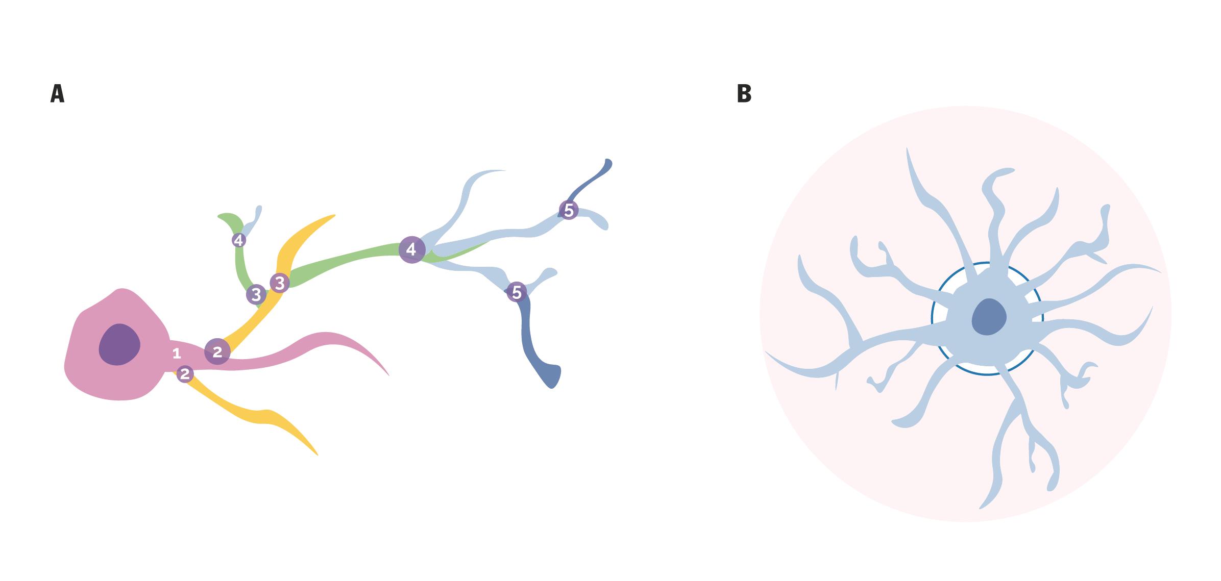
Figure 1. Graphical representation of dendrite branch level and dendrite volume. A. The numbers represent each ramification level, with each dendrite branch level distinguished by different colors for clear differentiation. B. The blue-shaded area (starting from the darker blue circle) highlights the dendrite volume, illustrating its distribution along the dendritic structure.
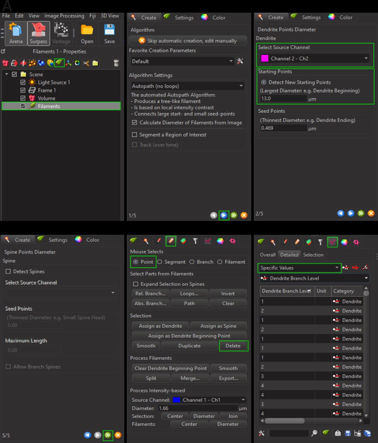
Figure 2. Three-dimensional reconstruction of microglial filaments. A. Select the leaf icon to initiate filament rendering. B. Click on the blue arrow to proceed to parameter adjustments. C. Choose the source channel and manually adjust the “largest diameter” value. D. De-select spine detection, then click the green double arrow to complete the reconstruction. E. Switch to the Pencil tab for editing filaments. F. Navigate to the Results tab and select the parameters of interest from the drop-down menu for further analysis.
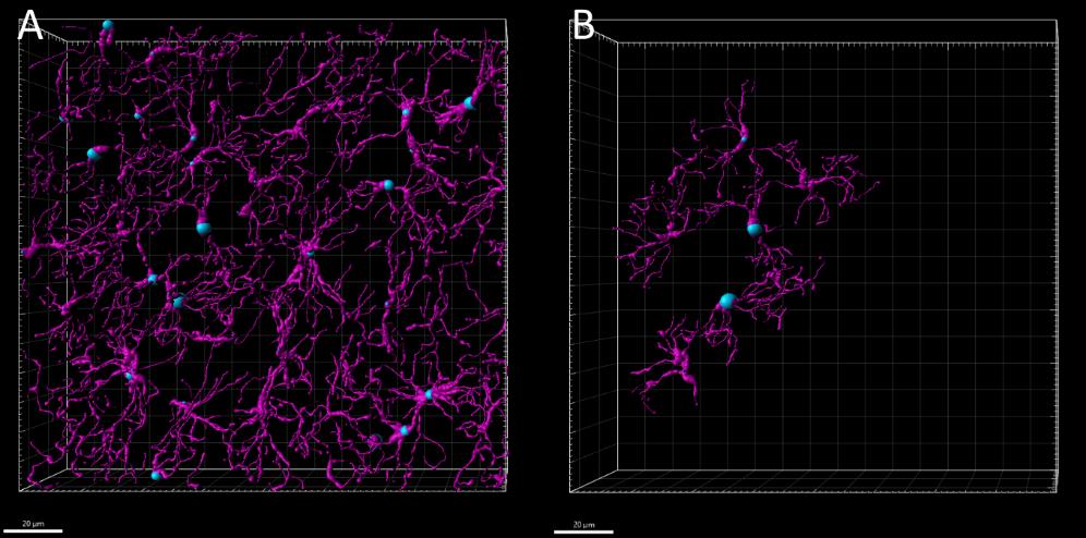
Figure 3. Three-dimensional editing of microglial filaments. Microglial cells located away from the tissue edges were selected for further editing. A. Filaments automatically reconstructed by Imaris software. B. Filaments post-editing, using surface rendering as a guide for accurate refinement.
3. Soma volume (Figures 4–5)
a. To create a surface, click on the blue gem icon.
b. In the panel below, choose “skip automatic creation, edit manually.”
c. Navigate through the Z-stacks to locate the soma of interest. Use the draw tool to trace the outline of the soma on at least three different levels.
Note: Ensure you select Z-stack slices that provide the clearest image of the soma.
d. Once done, click on create surface, and the software will generate and analyze the selected surfaces.
e. Navigate to the Results section, select the relevant parameters, and choose the measurement you require, such as soma volume.
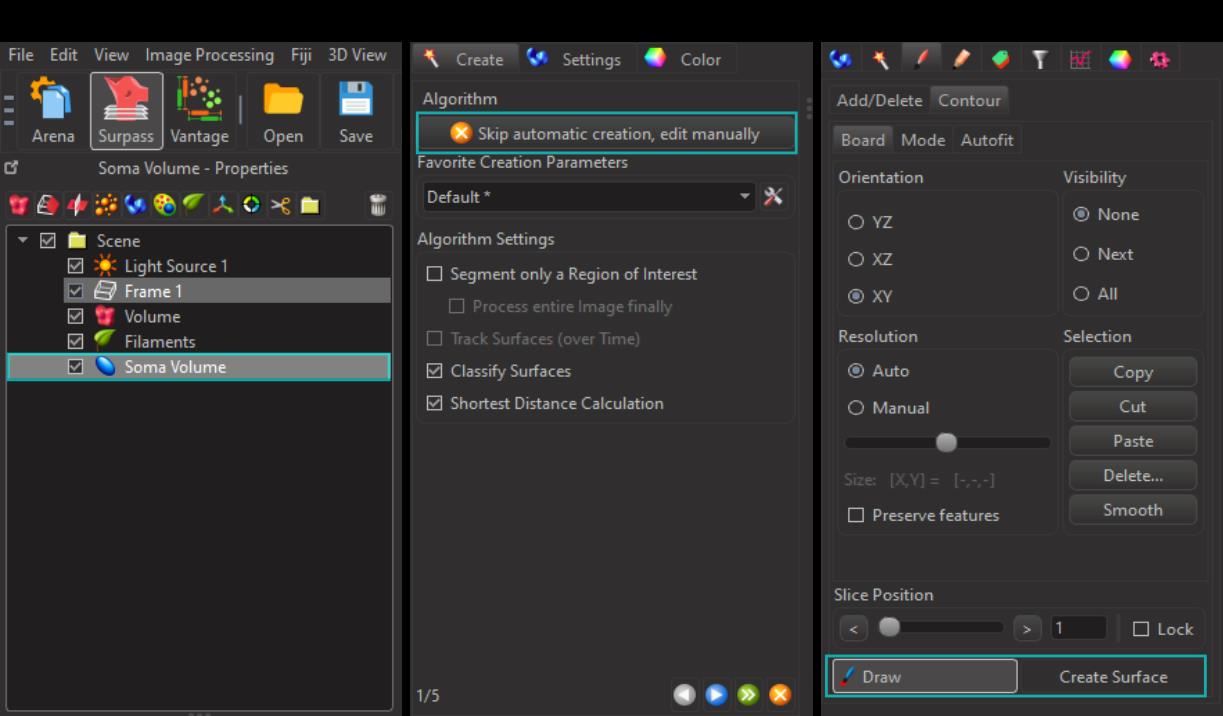
Figure 4. Three-dimensional reconstruction of soma volume of microglial cells. A. Select the surface rendering tool. B. Skip automatic creation and proceed with manual editing. C. Employ the draw tool to outline the microglial somas, then create the corresponding surfaces for volume analysis.
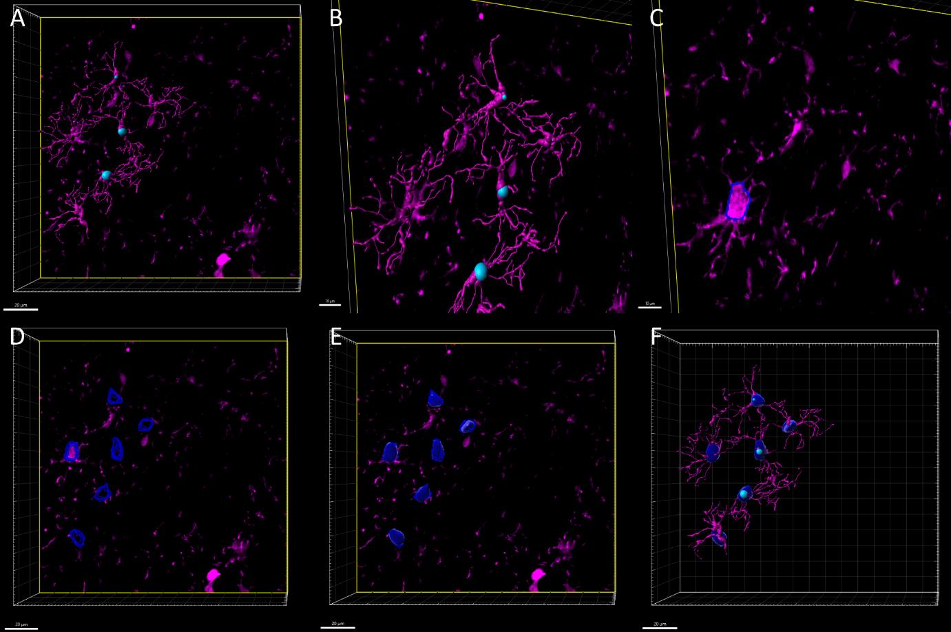
Figure 5. Three-dimensional reconstruction of microglial soma volume. Z-stack images of microglial cells labeled with the IBA1 antibody. A. Surface and filament rendering displaying the microglial cells selected for analysis. B. Magnified view of the region in panel A. C. Manual contouring of microglial somas (dotted blue lines) across individual slices of the Z-stack D. Merged soma contours from all Z-stack slices for the selected microglial cells. E. 3D reconstruction of microglial somas from the merged contours. F. Each reconstructed soma corresponds to a filament reconstruction, previously selected for analyses. Scale bars = 20 μm in A, D, E, F; 10 μm in B, C.
4. Imaris 3D surface (Figure 6 and Video 3)
a. Add a new Surface by clicking on the blue gem icon.
b. Click on the blue arrow to proceed, then select the channel of interest.
c. Adjust the Surfaces Detail parameter to increase or decrease surface precision.
Note: If the Smooth option is selected, surface detail will be calculated automatically. Manually increasing this value will reduce surface detail.
d. Manually adjust the Threshold (Absolute Intensity) parameter until the signal of interest is fully captured.
e. Modify the Filter Seed Point parameter to ensure all desired filaments are included.
f. Click Finish to complete the filament rendering.
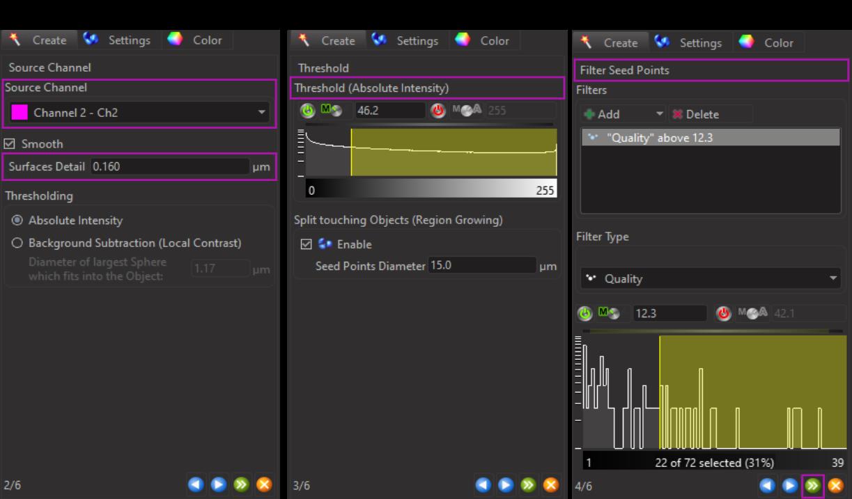
Figure 6. Three-dimensional reconstruction of microglial surfaces. A. Select the source channel and manually adjust the surface detail parameter. B. Adjust the threshold to ensure that all signals of interest are captured. C. Adjust the filter seed points to include the desired filaments in the final reconstruction.
Data analysis
Custom Python scripts were developed to facilitate the analysis of Imaris outputs. First, export the relevant .csv files containing the desired parameters from Imaris for further processing (Figure 7).
Note: Imaris generates two .csv files for each Z-stack, one containing dendrite volume data and the other containing branch-level data for the analyzed cells.
For each Z-stack .csv file, run the DendriteVolume.py and DendriteBranchLevel.py scripts as follows:
-To select specific output files for comparison:
python3 DendriteScript.py pathtocsvfile1 pathtocsvfile2 pathtocsvfile3 …
-To analyze all samples within a folder:
python3 DendriteScript.py pathtofolder/*
-If no input files are specified, the script will attempt to analyze all .csv files located in the same directory as the script.
The script will output the total dendrite volume (Dendrite Volume) and the total number of branches for each branch level (Dendrite Branch Level) for the same microglial cell (Filament ID).
1. Dendrite volume output: The first line displays the name of the .csv file (e.g., 2248a_zstack_40x_zoom1_Detailed.csv). Below this, two columns are presented: the first lists the microglial cell IDs, and the second shows the total dendrite volume.
2. Dendrite branch level output: Similarly, the first line shows the name of the .csv file (e.g., 2284a_zstack_40x_zoom1_Detailed.csv). The second line represents the Filament ID, followed by two columns: one for the branch level (with 1 representing the first branch from the soma) and another for the number of branches at each level.
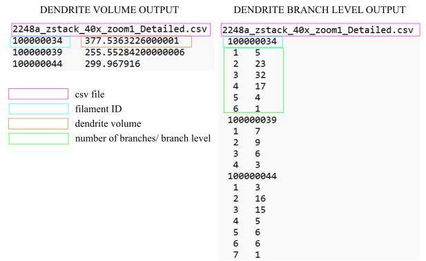
Figure 7. Output examples of dendrite volume and dendrite branch Level. The identifier 100000034 corresponds to one of the three microglial cells analyzed in the 2248a z-stack. The orange square indicates the total measured dendrite volume of the cell, while the green square represents the number of branches at each branch level (e.g., 5 branches for the first level, 23 branches for the second level).
Validation of protocol
This protocol has been used and validated in Figure 3f–j of the following research article:
Puighermanal, E. et al. [13]. Cannabidiol ameliorates mitochondrial disease via PPARγ activation in preclinical models. Nat Commun.
In this research article, we used the protocol described here to analyze 3D microglial morphology (Figure 8A) in the external globus pallidus, a highly affected brain region in Leigh syndrome mouse models. We demonstrated that mice with conditional Ndusf4 ablation in Gad2-espressing neurons exhibited morphometric remodeling of microglia resembling the activated phenotype. Specifically, microglial cells in mutant mice displayed a larger soma size (Figure 8B) and dendrite volume (Figure 8C) compared to control mice, along with fewer branch levels and fewer branches per level (Figure 8D). Total filament length was not altered (Figure 8E). Data represented in Figure 8 are extracted from Puighermanal et al. [13].
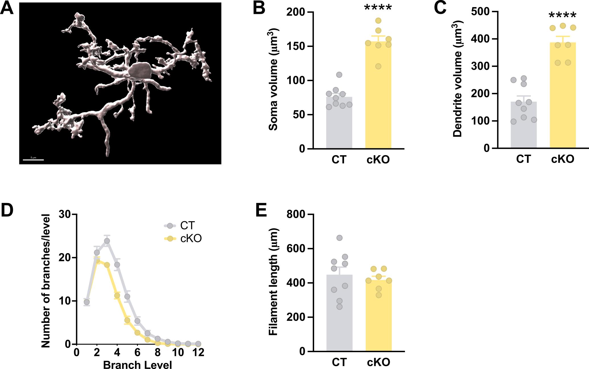
Figure 8. Morphometric analyses of microglia in a Leigh syndrome mouse model that courses with microgliosis. A. Imaris 3D surface reconstruction of a microglial cell. B. Quantification of soma volume/cell of IBA1+ cells (n = 9 control and 7 Gad2:Ndufs4cKO mice, two-sided t-test, ****p < 0.0001). C. Quantification of total dendrite volume/cell of IBA1+ cells (n = 9 control and 7 Gad2:Ndufs4cKO mice, two-sided t-test, ****p < 0.0001). D. Distribution plot of microglial ramification (n = 9 control and 7 Gad2:Ndufs4cKO mice, two-way ANOVA repeated measures, ****p < 0.0001). E. Quantification of total dendrite length/cell of IBA1+ cells (n = 9 control and 7 Gad2:Ndufs4cKO mice, two-sided t-test). All data are presented as mean values ± SEM. Veh vehicle, CT control mice, cKO Gad2:Ndufs4cKO mice. Scale bar: 8 μm.
General notes and troubleshooting
Troubleshooting
Problem 1: Densely packed cells make it difficult to reconstruct individual microglial filaments in 3D.
Possible cause: High cell density in the region of interest, especially in central areas of the sample and/or due to a neuroinflammatory environment, which increases microglial proliferation and clustering.
Solutions:
1. Select regions with more isolated cells for imaging. Focus on peripheral areas of the sample where cell density is typically lower.
2. Manually exclude overlapping or crowded cells during analysis by erasing them in Imaris. This approach allows for a cleaner reconstruction of the remaining cells.
3. In samples with neuroinflammation, consider imaging regions with lower microglial density to reduce complexity in filament reconstruction.
Problem 2: Differences in intensity and morphology of microglial cells between experimental groups impact imaging consistency.
Possible cause: Confocal settings (e.g., laser power, gain, offset) optimized for one group may not work well for others due to condition-dependent variability.
Solutions:
1. Test and optimize imaging parameters (e.g., laser intensity, detector gain) across all experimental groups before starting batch imaging.
2. Adjust settings to achieve a balance that provides consistent signal-to-noise ratios and preserves cell morphology across conditions.
Acknowledgments
The authors apologize to any colleagues whose work was not discussed in this paper. The authors greatly thank the Microscopy Imaging Platform at Autonomous University of Barcelona for continuous technical support with the Imaris software and Kevin Aguilar for technical advice.
This work was supported by the MINECO Ramon y Cajal (RYC2020-029596-I) and MICINN (PID2021-125079OA-I00) grants awarded to E.P., as well as the 2024 FI-100645 fellowship granted to G.vdW.
Author Contributions
E.P. and M.dD conceptualized and planned the study. M.dD performed immunofluorescence studies and image analysis. A.dD. and M.dD. created the data analysis pipeline and analyzed the pertaining data, A.K. generated, rendered and edited the final audiovisual content reported. M.dD., A.K., and E.P. wrote the manuscript. G.vdW. edited the manuscript.
Competing interests
The authors declare no conflict of interest.
Ethical considerations
All animal experiments were performed with the approval of the ethical committee at Autonomous University of Barcelona (CEEAH) and Generalitat de Catalunya (DMAH).
References
- Aguilar, K., Comes, G., Canal, C., Quintana, A., Sanz, E. and Hidalgo, J. (2022). Microglial response promotes neurodegeneration in the Ndufs4 KO mouse model of Leigh syndrome. Glia. 70(11): 2032–2044. https://doi.org/10.1002/glia.24234
- Lee, J. W., Chun, W., Lee, H. J., Kim, S. M., Min, J. H., Kim, D. Y., Kim, M. O., Ryu, H. W. and Lee, S. U. (2021). The Role of Microglia in the Development of Neurodegenerative Diseases. Biomedicines. 9(10): 1449. https://doi.org/10.3390/biomedicines9101449
- Leyh, J., Paeschke, S., Mages, B., Michalski, D., Nowicki, M., Bechmann, I. and Winter, K. (2021). Classification of Microglial Morphological Phenotypes Using Machine Learning. Front Cell Neurosci. 15: e701673. https://doi.org/10.3389/fncel.2021.701673
- Doorn, K. J., Goudriaan, A., Blits‐Huizinga, C., Bol, J. G., Rozemuller, A. J., Hoogland, P. V., Lucassen, P. J., Drukarch, B., van de Berg, W. D., van Dam, A., et al. (2013). Increased Amoeboid Microglial Density in the Olfactory Bulb of Parkinson's and Alzheimer's Patients. Brain Pathol. 24(2): 152–165. https://doi.org/10.1111/bpa.12088
- Green, T. R. F., Murphy, S. M. and Rowe, R. K. (2022). Comparisons of quantitative approaches for assessing microglial morphology reveal inconsistencies, ecological fallacy, and a need for standardization. Sci Rep. 12(1): e1038/s41598–022–23091–2. https://doi.org/10.1038/s41598-022-23091-2
- Clarke, D., Crombag, H. S. and Hall, C. N. (2021). An open-source pipeline for analysing changes in microglial morphology. Open Biol. 11(8): e210045. https://doi.org/10.1098/rsob.210045
- Heindl, S., Gesierich, B., Benakis, C., Llovera, G., Duering, M. and Liesz, A. (2018). Automated Morphological Analysis of Microglia After Stroke. Front Cell Neurosci. 12: e00106. https://doi.org/10.3389/fncel.2018.00106
- Verdonk, F., Roux, P., Flamant, P., Fiette, L., Bozza, F. A., Simard, S., Lemaire, M., Plaud, B., Shorte, S. L., Sharshar, T., et al. (2016). Phenotypic clustering: a novel method for microglial morphology analysis. J Neuroinflammation. 13(1): 153. https://doi.org/10.1186/s12974-016-0614-7
- York, E. M., LeDue, J. M., Bernier, L. P. and MacVicar, B. A. (2018). 3DMorph Automatic Analysis of Microglial Morphology in Three Dimensions fromEx VivoandIn VivoImaging. eNeuro. 5(6): ENEURO.0266–18.2018. https://doi.org/10.1523/eneuro.0266-18.2018
- Gavrin, A. and Fedorova, E. (2015). Quantification of the Volume and Surface Area of Symbiosomes and Vacuoles of Infected Cells in Root Nodules of Medicago truncatula. Bio Protoc. 5(23): e1665. https://doi.org/10.21769/bioprotoc.1665
- Ohnishi, Y. and Okamoto, T. (2015). Microscopic Observation, Three-dimensional Reconstruction, and Volume Measurements of Sperm Nuclei. Bio Protoc. 5(7): e1437. https://doi.org/10.21769/bioprotoc.1437
- Bolea, I., Gella, A., Sanz, E., Prada-Dacasa, P., Menardy, F., Bard, A. M., Machuca-Márquez, P., Eraso-Pichot, A., Mòdol-Caballero, G., Navarro, X., et al. (2019). Defined neuronal populations drive fatal phenotype in a mouse model of Leigh syndrome. eLife. 8: e47163. https://doi.org/10.7554/elife.47163
- Puighermanal, E., Luna-Sánchez, M., Gella, A., van der Walt, G., Urpi, A., Royo, M., Tena-Morraja, P., Appiah, I., de Donato, M. H., Menardy, F., et al. (2024). Cannabidiol ameliorates mitochondrial disease via PPARγ activation in preclinical models. Nat Commun. 15(1): 7730. https://doi.org/10.1038/s41467-024-51884-8
- Franklin, K. and Paxinos, G. (2007). The mouse brain in stereotaxic coordinates. 2nd edn. Elsevier, Amsterdam.
- Puighermanal, E., Cutando, L., Boubaker-Vitre, J., Honoré, E., Longueville, S., Hervé, D. and Valjent, E. (2016). Anatomical and molecular characterization of dopamine D1 receptor-expressing neurons of the mouse CA1 dorsal hippocampus. Brain Struct Funct. 222(4): 1897–1911. https://doi.org/10.1007/s00429-016-1314-x
- Biever, A., Puighermanal, E., Nishi, A., David, A., Panciatici, C., Longueville, S., Xirodimas, D., Gangarossa, G., Meyuhas, O., Hervé, D., Girault, J.-A., & Valjent, E. (2015). PKA-dependent phosphorylation of ribosomal protein S6 does not correlate with translation efficiency in striatonigral and striatopallidal medium-sized spiny neurons. J Neurosci. 35(10): 4113–4130. https://doi.org/10.1523/JNEUROSCI.3288-14.2015
Article Information
Publication history
Received: Oct 16, 2024
Accepted: Jan 8, 2025
Available online: Jan 26, 2025
Published: Feb 20, 2025
Copyright
© 2025 The Author(s); This is an open access article under the CC BY-NC license (https://creativecommons.org/licenses/by-nc/4.0/).
How to cite
de Donato, M. H., Kouchaeknejad, A., de Donato, A., Van Der Walt, G. and Puighermanal, E. (2025). Streamlined Quantification of Microglial Morphology in Mouse Brains Using 3D Immunofluorescence Analysis. Bio-protocol 15(4): e5218. DOI: 10.21769/BioProtoc.5218.
Category
Bioinformatics and Computational Biology
Neuroscience > Cellular mechanisms > Microglia
Cell Biology > Cell-based analysis
Do you have any questions about this protocol?
Post your question to gather feedback from the community. We will also invite the authors of this article to respond.