- Protocols

- Articles and Issues
- For Authors
- About
- Become a Reviewer

Model Architecture Analysis and Implementation of TENET for Cell–Cell Interaction Network Reconstruction Using Spatial Transcriptomics Data
(*contributed equally to this work, § Technical contact: yujianlee1119@gmail.com) Published: Vol 15, Iss 3, Feb 5, 2025 DOI: 10.21769/BioProtoc.5205 Views: 1444
Reviewed by: Prashanth N SuravajhalaAYŞE NUR PEKTAŞAnonymous reviewer(s)
Original research article
The authors used this protocol in:
Mar 2024
Advertisement


Protocol Collections
Comprehensive collections of detailed, peer-reviewed protocols focusing on specific topics


Related protocols
Abstract
Cellular communication relies on the intricate interplay of signaling molecules, which come together to form the cell–cell interaction (CCI) network that orchestrates tissue behavior. Researchers have shown that shallow neural networks can effectively reconstruct the CCI from the abundant molecular data captured in spatial transcriptomics (ST). However, in scenarios characterized by sparse connections and excessive noise within the CCI, shallow networks are often susceptible to inaccuracies, leading to suboptimal reconstruction outcomes. To achieve a more comprehensive and precise CCI reconstruction, we propose a novel method called triple-enhancement-based graph neural network (TENET). The TENET framework has been implemented and evaluated on both real and synthetic ST datasets. This protocol primarily introduces our network architecture and its implementation.
Key features
• Cell–cell reconstruction network using ST data.
• To facilitate the implementation of a more holistic CCI, we incorporate diverse CCI modalities into consideration.
• To further enrich the input information, the downstream gene regulatory network (GRN) is also incorporated as an input to the network.
• The network architecture considers global and local cellular and genetic features rather than solely leveraging the graph neural network (GNN) to model such information.
Keywords: Cell–cell interaction network (CCI) reconstructionGraphical overview
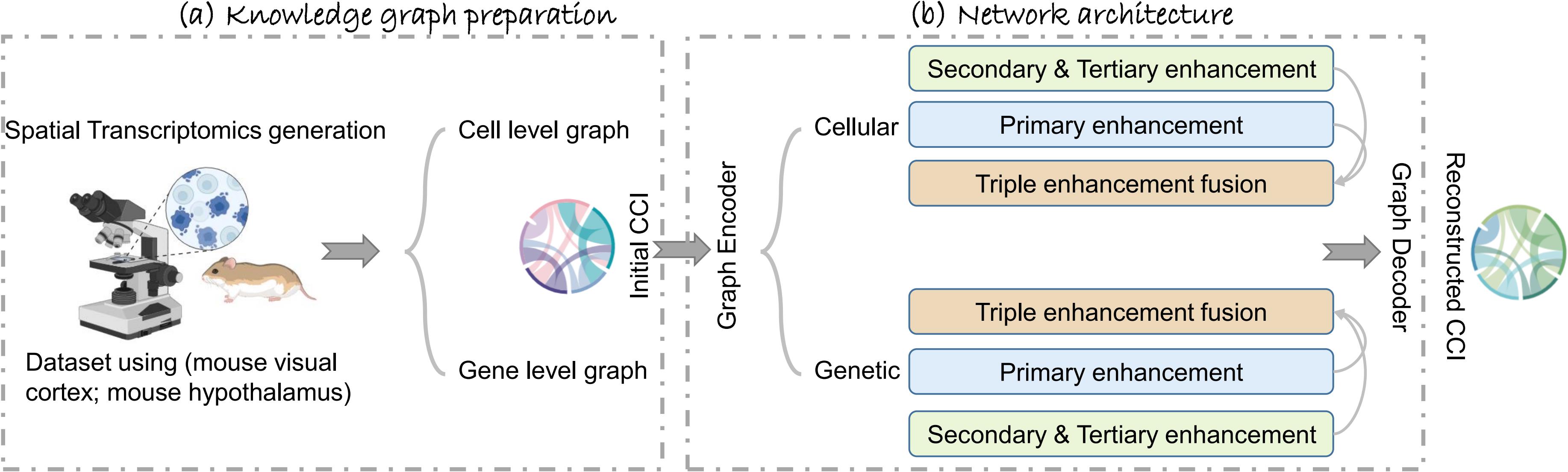
Graphical abstract of TENET, including (a) the knowledge graph preparation on both cell and gene levels and (b) the network architecture.
Background
Understanding cellular communication is crucial for constructing a cell–cell interaction network (CCI), which allows researchers to investigate the roles of different cells in biological processes and diseases. A common method for analyzing CCI involves studying the interactions between secreted ligands and their corresponding receptors (LR pairings), as these interactions are essential for signal transmission.
However, CCIs also occur through direct cell–cell contact, the extracellular matrix (ECM), and the secretion of signaling molecules [1]. Focusing solely on LR pairings overlooks the spatial context in which these interactions occur. With the advent of spatial transcriptomics (ST) data, incorporating spatial information can help address this limitation. Several methods for reconstructing CCI using ST data have been developed. For instance, Giotto [2] constructed a spatial grid based on cell coordinates to model proximal interactions but did not account for distal interactions. MISTy [3] utilizes multiple perspectives (intrinsic, local, tissue) to enhance cell knowledge for CCI inference. DeepLinc [4] employs a graph neural network (GNN) [5] to create a spatial proximity graph, using KNN [6] to identify both proximal and distal interactions. Despite these advances, modeling ST data solely at the cell level can lead to false positives and negatives due to a lack of downstream information. Incorporating downstream data, such as intracellular signaling, gene regulation, and protein changes can provide crucial insights for understanding actual CCI; CLARIFY [7] combines cellular and genetic information to build knowledge graphs for GNN inputs, effectively capturing structural features important for CCI inference. However, solely using GNNs is limiting, as they often aggregate local information, hindering the capture of global context. GNNs also struggle with similar nodes, which may lead to a loss of features’ specificity.
To overcome these challenges, we propose a novel approach called triple-enhancement-based graph neural network (TENET), designed as a comprehensive architecture for CCI reconstruction. TENET employs a graph convolution network (GCN) [8] backbone to extract global features from the data at multiple resolutions, generating robust latent feature embeddings. These embeddings then undergo a triple-enhancement mechanism that restores cell specificity that may have been lost during the GCN's global aggregation. The first enhancement mitigates the GCN's over-smoothing problem, while the secondary and tertiary enhancements refine the embeddings both locally and globally. Finally, a denoising loss function is introduced to tackle the challenges posed by noisy, low-quality data often encountered in small molecule experiments. This multi-scale enhancement strategy enables TENET to accurately and robustly reconstruct cell–cell interactions, addressing the limitations of previous methods and opening new avenues for researchers to explore the complexities of CCI.
Software and datasets
Software1. 2.90 GHz Intel i7-10700F CPU and NVIDIA A100 graphics card; nvcc: NVIDIA (R) Cuda compiler driver; Copyright 2005–2024 NVIDIA Corporation; Built on Tue_Feb_27_16:19:38_PST_2024; Cuda compilation tools, release 11.7, V11.7.99; Build cuda_11.7.r11.7/compiler.33961263_0
Input data
1. Three ST datasets are utilized, namely seqFISH, MERFISH, and scMultiSim [9], which can be acquired at https://bitbucket.org/qzhu/smfish-hmrf/src/master/, https://datadryad.org/stash/dataset/10.5061/dryad.8t8s248, and https://github.com/ZhangLabGT/scMultiSim. The hyperlinks direct to the datasets utilized in TENET. The specific analysis of the datasets is mentioned in the following sections.
Procedure
The procedure includes two parts: the input preparation in section A and the network architecture in section B. The inputs of the network are the knowledge graphs from the cell and gene levels. Graphs encapsulate both the nodal feature representation V as well as the corresponding adjacency matrix (edge list) Adj. In section A, we elucidate the respective construction for the cell-level graph and the gene-level graph, denoted as Gc and Gg, respectively. In section B, we present the corresponding operations to the constructed knowledge graphs. Table 1 lists the frequently used symbols in sections A and B, improving overall readability.
Table 1. Frequently used symbols
| Symbol | Explanation |
|---|---|
| Gc(g) =(Vc(g) ,Adjc(g)) | Input cell (gene) knowledge graph, containing nodes with features and the adjacency matrix. |
| Vc(g) ∈R(Nc(g) ×Fc(g)) | Nc(g) number of nodes with Fc(g) feature dimensions. |
| Adjc(g) ∈R(Nc(g) ×Nc(g)) | Adjacency matrix representing the establishment of interactions among nodes. |
| Kp | The numbers of cells' indexes denoting the establishment of proximal interaction. |
| Adjp∈R(Nc×Nc) | The proximal interaction adjacency matrix. |
| Kir | The numbers of cells' indexes denoting the establishment of intermediate range interaction. |
| Adjir∈R(Nc×Nc) | The intermediate range interaction adjacency matrix. |
| Zc(g) ∈R(Nc(g) × Fc(g)) | Latent feature embeddings after the input graph Gc(g) traverse through the GCN encoder. |
| Z(c+g)∈R(Nc×F(c+g)) | An integration of Zc and Zg. |
| Z'(c+g)∈R(Nc×F'(c+g)), Z'g∈R(Nc×F'g) | Enhancing Z(c+g), Zg using CECB. |
| Z''(c+g)∈R(Nc×F''(c+g)), Z'g∈R(Nc×F''g) | Enhancing Z(c+g)' and Zg' using EEB and SEB, respectively. |
| Z'''(c+g)∈R(Nc×F'''(c+g)), Z'g∈R(Nc×F'''g) | Integration of the previous result {Z(c+g), Z(c+g,)' Z(c+g)'''},{Zg, Z(g,)' Zg'''}. |
A. Input preparation
The construction of Gc and Gg is described in subsections a and b, respectively.
1. Cell-level graph construction
From the aforementioned links, there are four .csv files corresponding to each dataset. These files encompass the spatial coordinates of individual cells, the cell type classifications, the gene expression count matrices for each cell, and the adjacency matrix delineating cellular connectivity. Except for the adjacency matrix file, the other three files are encapsulated into a data frame, representing the cells' features. Figure 1 depicts the cell features organized into a data frame format; using the seqFISH dataset as an example, there are Nc number of cells with Fc number of features, denoted as Vc∈R(Nc×Fc). In this feature representation, the blue overlay delineates the spatial coordinates of individual cells, the green overlay denotes the cell type classifications, and the red overlay represents the gene expression matrix. (Due to space limitation, the red overlay is a partial visualization of the gene expression profile.) To build a cell-level adjacency matrix Adjc, our procedure is not simply to use the provided adjacency matrix but to simulate actual cell communication in the real biological world by integrating the three interaction modes into consideration. These three secretion modes exhibit a different range of interactions, where the cell–cell direct contact is defined to be the proximal interaction, ECM to be the intermediate interaction, and the secreting signaling molecule to be the distal interaction. Given that our approach is based on the neighbor search algorithm and that the input data consists solely of the spatial coordinates of the cells, considering the distal interaction will introduce error to the constructed CCI. Therefore, the initial CCI includes the proximal and intermediate-range interaction modes, and our algorithm combines two neighbor clustering methods, both of which have different purposes. The first is the hierarchical navigable small world (HNSW) algorithm [10], which is good at processing large numbers of data points and speeding up the construction of our spatial connectivity networks. The second is the Louvain algorithm [11], which can merge small clusters into larger ones, helping the search for intermediate-range cellular interactions. The implementations are summarized as follows:
Finding proximal interacting cells Kp.
Finding intermediate-range interacting cells Kir.
Integration of the initial CCI.
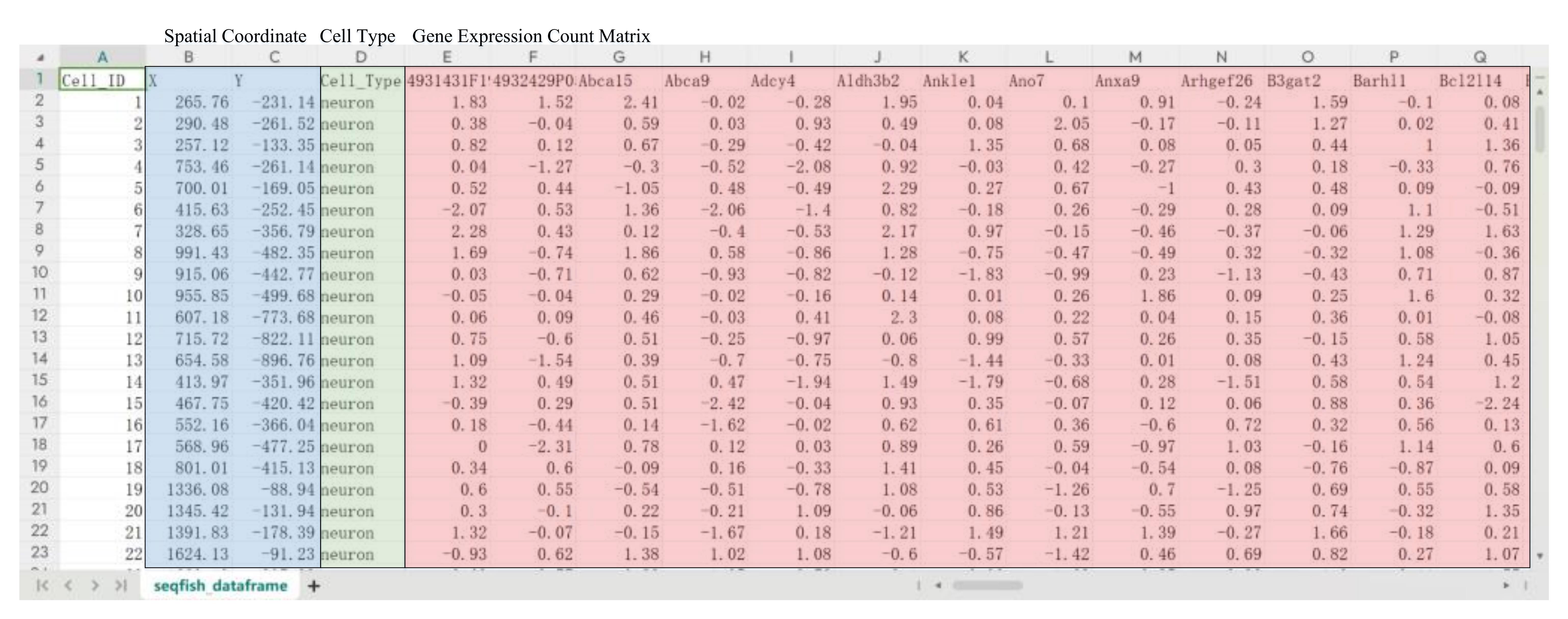
Figure 1. Demonstration of the seqFISH cell data features, where the blue overlay delineates the spatial coordinates of individual cells, the green overlay denotes the cell type classifications, and the red overlay represents the gene expression levels within each cell.
It is highly recommended that researchers combine Algorithm 1 with Figure 2 for a better understanding.
| Algorithm 1: Construction of the cell adjacency matrix |
|---|
Input: Cell spatial coordinates Output: Cell adjacency matrix Step 1: Find Kp proximal interacting cells. 1.1 Construct the spatial connectivity network. 1.2 kNNquery indexing Kp. 1.3 Form the proximal interaction adjacency matrix Adjp: [[N1, N2, …, Nc]1,[N1, N2, …, Nc]2,…[N1, N2, …, Nc](Nc) ] Step 2: Find 2.1 Coalesce small clusters into a larger cluster. , (1) 2.2 Iterate until ∆Q converge indexing. 2.3 Form the inter-mediate range interaction adjacency matrix Adjir. Step 3: Construct the cell adjacency matrix Adjc by combining Adjp, Adjir. |
In Algorithm 1, in step 1.1, based on the input coordinates of the cells, a spatial connectivity network is constructed using the spatial proximity and geometric relationship. The result is shown in Figure 2A. The subsequent kNNquery in step 1.2 uses the spatial connectivity network to find Kp proximal interacting cells, defined as having potential direct cell–cell contact with the query cell. The green circle in Figure 2B is a demonstration of the randomly selected cell (red dot) and its interacting entities. The output of step 1 is the proximal interaction adjacency matrix Adjp∈R (Nc×Nc), where Nc is denoted as the number of input cells, the corresponding Kp index is 1, and the others are 0. Step 2 is the construction of the intermediate range interaction adjacency matrix. In step 2.1, the process involves grouping each cell with its neighbors and evaluating whether the maximum gain of modularity (∆Q) is greater than 0. If the gain is positive, the cell is assigned to the adjacent cell with the largest modular increment. Step 2.2 is the iteration of step 2.1, until ∆Q in Eq. (1) in Algorithm 1 no longer changes, being defined to be convergence. The result indicates that the cells within the same community are identified as potentially having intermediate-range interactions (ECM) with respect to the query cell, denoted as Kir. As a result, the number of potential interacting cells is Kp + Kir. The green circle in Figure 3C is the demonstration of a randomly picked cell (red dot) with its proximal interacting cells Kp and intermediate-range interacting cells Kir (green dots). In step 3, we can construct the adjacency matrix by
, (2)
on the cell level, denoting whether two cells will establish interactions under the conditions of Adjp and Adjir. Then, the cell-level graph Gc can be constructed using Vc and Adjc.
In summary, Algorithm 1 distinguishes itself from the existing approaches relying on the kNN method, in which only
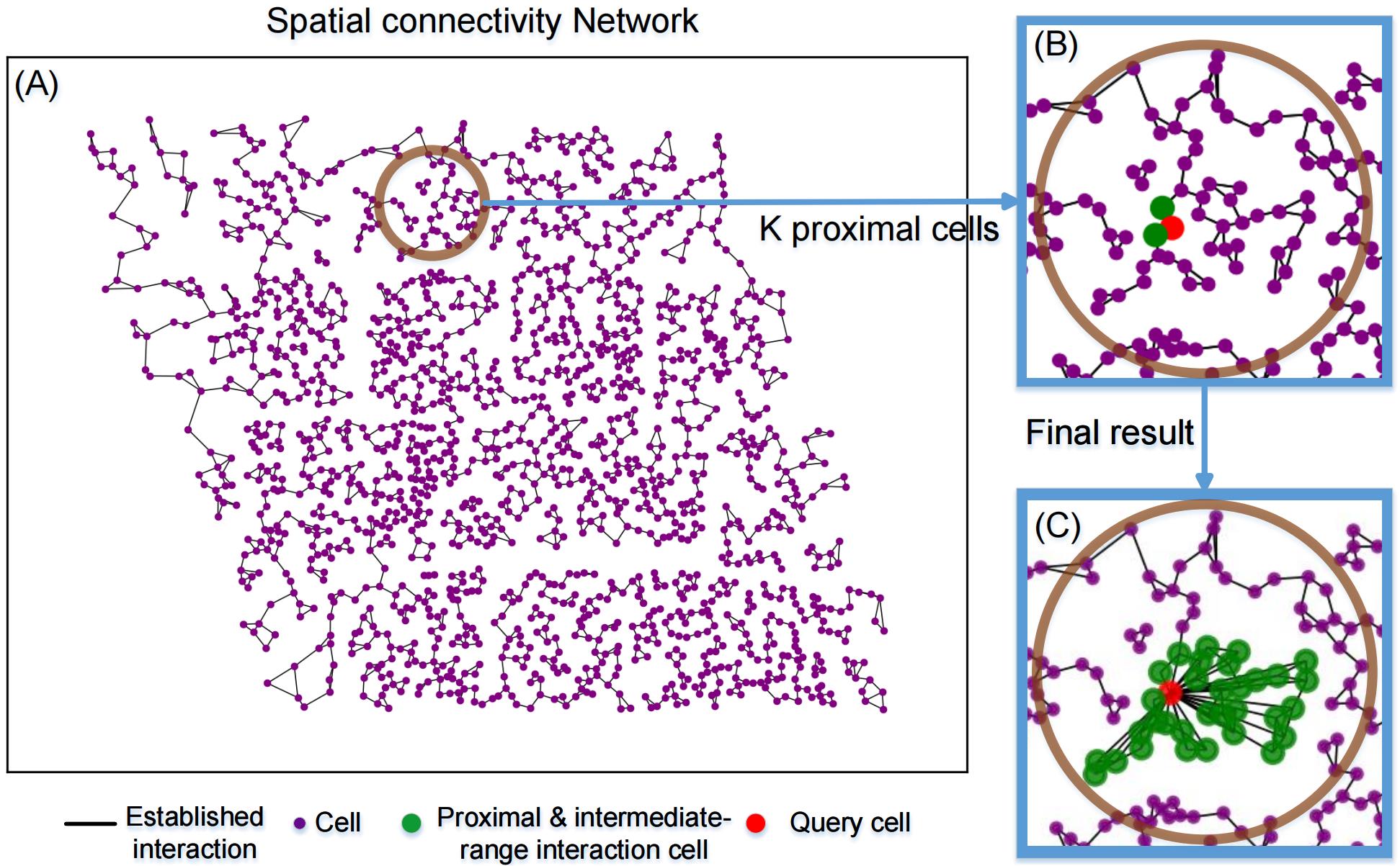
Figure 2. Demonstration of the initial CCI construction using the seqFISH dataset. A. The purple dots represent the spatial locations of cells, and the spatial connectivity network generates the linkages between them. B. After step 1 in Algorithm 1, the randomly selected cell is in red in our demonstration, Kp (Kp = 2) returns in green and in the same size as the query cell does, denoted as the proximal interacting cells. (C) Cells in green inside the green circle (Kp+Kir) are defined to have potential interactions with the query cell in red, denoted as the proximal and intermediate-range interacting cells.
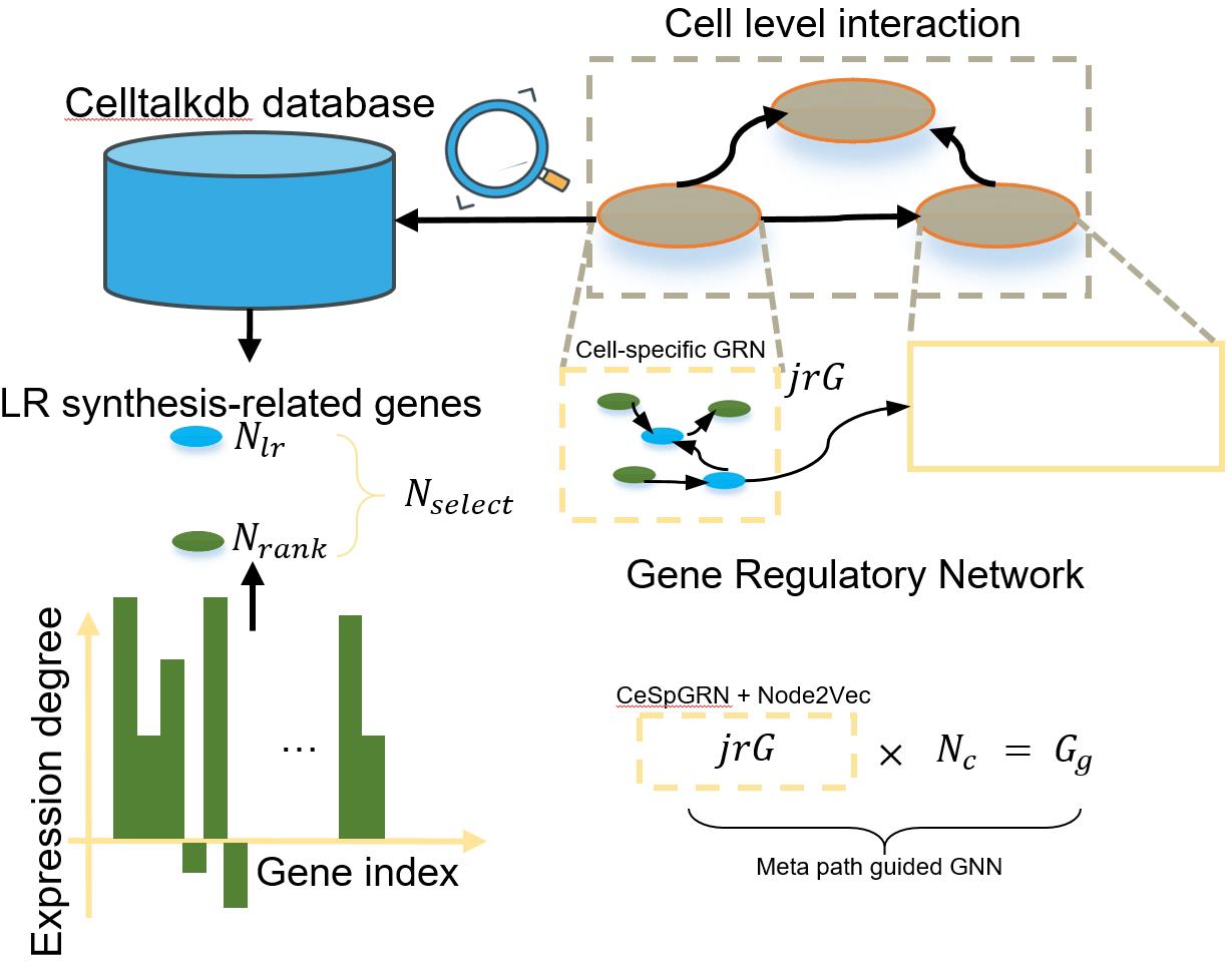
Figure 3. Construction process of Gg
2. Gene-level graph construction
The construction of the gene-level graph Gg is presented in Figure 3 and involves two main steps:
a. Construction of the cell-specific GRN:
Select Nselect (Nselect= Nlr+ Nrank) genes, comprising Nlr genes related to LR synthesis using standardized LR databases provided by Celltalkdb [14] and Nrank highly expressed genes.
Use the CeSpGRN backbone [15] to obtain the cell-specific gene interaction network, represented as cell-specific gene adjacency matrices (Nc graphs).
Apply Node2Vec [16] to generate features Fselect for the selected genes in each cell-specific graph.
b. Construction of the global GRN:
Combine the cell-specific graphs (NcjrG) into a global gene graph Gg.
Enrich the gene features by preserving the connections from the cell-specific graphs and using a meta-path-guided graph neural network [17,18] to derive new features F'select.
The final gene features Fg in Gg are obtained by integrating Fselect and F'select.
Researchers can use the following links to customize the gene level graph: https://github.com/PeterZZQ/CeSpGRN, https://github.com/eliorc/node2vec, and https://github.com/zhiqiangzhongddu/PM-HGNN.
B. Network architecture
Triple-enhancement-based graph neural network (TENET) is an end-to-end structure that could be utilized to retrieve ST data features as well as the graph structure to learn and reproduce. Gc and Gg are separately encoded in the graph convolution network (GCN) encoder in the first stage, obtaining the latent feature embeddings, denoted as Zc and Zg. Zg will traverse through the channel enhancement compensation block (CECB) and synergistic enhancement block (SEB). Before Zc moves on to the next stage, we integrate Zc and Zg to become Z(c+g). Then, Z(c+g) will traverse through CECB and the elective enhancement block (EEB). The whole process is illustrated in Figure 4.
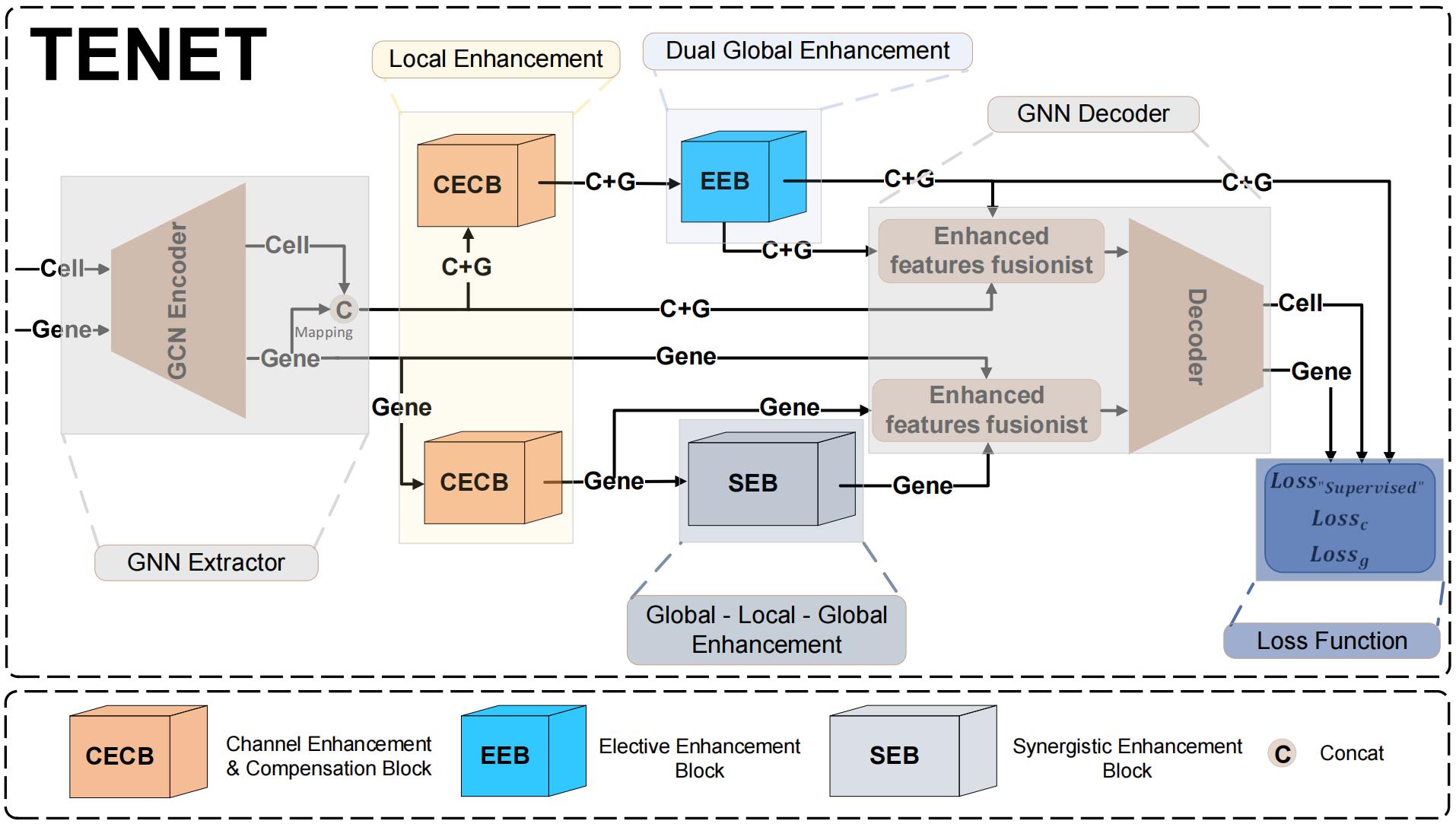
Figure 4. TENET workflow. The GCN encoder extracts latent feature embeddings Zc and Zg from Gc and Gg. Before Zc is input into the subsequent blocks, we have an integration process converting Zc into Z(c+g). The subsequent triple-enhancement mechanism can be summarized as local-global-local enhancement. By doing so, the network can not only extract feature representations from the node itself but also from the graph structure. Before the decoding process, we fuse the latent feature embeddings from the enhanced block to have an accumulated effect. For the loss function, we employ the binary cross entropy (BCE) loss function for both cell and gene. Besides, due to the utilization of the triple-enhancement mechanism, if the model is to be subjected to noise or wrongly enhanced during the enhancement process, which is undesirable, it would struggle to converge. Consequently, we have the Loss"supervised" function that enables the model to combat noise and enhance its resilience effectively.
1. GCN encoder
The core of TENET's architecture is built upon the GCN [8], which serves as the foundation for extracting meaningful node representations from the input graph Gc and Gg and outputs the latent feature embeddings of cells and genes denoted as Zc and Zg, respectively. The calculation process of the two-layer GCN encoder is presented as
(3)
In Eq. (3), the nonlinear activation function ReLU introduces nonlinearity into the node representations. is the degree of each node. is denoted as the adjacency matrix with self-loop (a linkage connected to the node itself). is denoted as the features extracted from the last layer; specifically, if layer = 0, are the original node features. is the learnable weight matrix from the previous layer, enabling the model to learn feature-specific transformations and effectively aggregate information from a node's local neighborhood. When inputting Zc to the next block, we first convert it into Z(c+g), introducing cross-resolution embedding to extend the model's ability to capture different data patterns.
2. Channel enhancement and compensation block (CECB)
The CECB in Algorithm 2 is a streamlined transition block; Z(c+g) and Zg are enhanced in the channel dimension, aiming to emphasize the relevant feature embeddings and mitigate the over-smoothing problem caused by the GCN encoder [19].
| Algorithm 2. Channel enhancement and compensation block (CECB) |
|---|
Input: Input feature: Z(c+g), Zg; Operation: Normalization: Batch normalization (BN), Activation function (ϕ,ω); Two fully connected layers [FC1, FC2]. Output: Z'(c+g), Z'g The results of the intermediate operations are represented using “temp” followed by different subscripts. if Z(c+g) Endif if temp(c+g)4 else
Endif return Output: Z'(c+g), Z'g |
3. Synergistic enhancement block (SEB)
The enhancement of Z'g in the SEB is done jointly by the global branch enhancement and the local branch enhancement. In Algorithm 3, the global branch enhancement utilizes the graph attention network (GAT) [20], and the local branch enhancement acts as a buffer to integrate the feature embeddings extracted from the GAT.
| Algorithm 3. Synergistic enhancement block (SEB) |
|---|
Input: Input features:Z'g; Operation: Graph Attention Network (GAT), Convolution (Conv1), Batch normalization (BN), Activation function (ϕ,σ); Linear transformation (MLP, contains three fully connected layers [FC3,FC4,FC5]); Kernel list: K [1, 3, 5]; Group Size: G; Latent dimension: Lg1,Ll ,Lg2; Storage list: sl = []; Attention weight list: awl []. Output: Z''g The result of the intermediate operations are represented using “global” / “local” followed by different subscripts. Global enhancement operation: Local enhancement operation: for k in K do: sl.append (localk) End for localfeature=stack(sl). The feature dimension turns into localenhance ϵ RNg×Ll. Global enhancement operation:
The feature dimension turns into globalenhance2 ϵ RNg×(Lg1*attention heads) return Output: Z''g = globalenhance2. |
4. Elective enhancement block (EEB)
The EEB in Algorithm 4 amplifies the latent feature embeddings by augmenting the spatial dimensions and leveraging adaptive feature selection [21], thereby bolstering the richness and caliber of the embeddings. The adaptive enhanced feature election mechanism in EEB bears a resemblance to the local branch in SEB.
| Algorithm 3. Elective enhancement block (EEB) |
|---|
Input: Input features: Z'(c+g); Operation: Adaptive average pooling(AAP), Convolution (Conv2,Conv3), Batch normalization (BN), Activation function (θ,ω); Two fully connected layers [FC6,FC7]); Latent dimension: L. Output: Z''(c+g) The results of the intermediate operations are represented using “temp” followed by different subscripts. The feature dimension turns into temp6 ϵ RNC×L. temp9= ω(FC6(Conv3 (temp7))), temp10= ω(FC6(Conv3(temp8))). The feature dimension turns into temp10 ϵ RNC×F''c+g. return Output: Z''c+g = FC7 (Z'c+g) * temp9*temp10. |
5. Triple-enhancement fusionist decoder (TEFD)
Triple-enhancement fusionist decoder (TEFD) fuses the enhanced latent feature embeddings from the previous blocks as input to the inner product decoder [22]. The two decoders for cell and gene are parallel, denoted as
Fusionc=sum(Zc+g, Z'c+g, Z''c+g). (4)
Fusiong=sum(Zg, Z'g, Z''c+g). (5)
The first terms in Eq. (4) and Eq. (5) Z(c+g) and Zg represent the raw latent feature embeddings obtained from the GCN encoder in subsection a. The second terms Z'(c+g) and Z'g undergo the CECB (primary enhancement) in subsection b. The third term Z''g is dual enhanced embeddings from SEB (secondary enhancement and tertiary enhancement) in subsection c. Analogously, Z''(c+g) is also a dual enhanced embedding when exported from EEB (secondary enhancement and tertiary enhancement) in subsection d. Each enhancement module incrementally amplifies inherent feature embeddings across different scales by progressively augmenting the channel dimensions, leading to a cumulative effect in Fusionc(g). To integrate the fusion features a step further, we have
Z'''c(g)= FC9(ReLU(FC8(Fusionc(g)))). (6)
Such a process discerns and extracts the salient features crucial for the subsequent decoding process.
The decoding process of Dc and Dg are summarized as follows: . The usage of the sigmoid activation is to limit the interaction scores between 0 and 1, representing the probability of the existence of an interaction between the corresponding cells (genes). Generally, TEFD ensures the interconnection and information flow among the blocks. The output of each block not only serves as input for the subsequent enhancement block but also contributes to the final reconstruction of CCI. By incorporating multi-scale information, a more nuanced understanding of cellular (genetic) interacting patterns can be achieved, allowing for a more accurate determination of communication establishment among cells.
6. Loss function
We employ the binary cross entropy (BCE) loss and propose a supervised loss in Algorithm 4. The BCE loss can achieve refinement in both the cell graph and gene graph and encourages the production of well-calibrated probabilities by penalizing large errors in the predicted probabilities [23].
To further correctly augment cell features, we have the supervised loss (Loss"supervised"). The inputs are the output of EEB and the output of the GCN encoder (after mapping and concatenating), the Z'(c+g) and Z(c+g), respectively, and its core concept is using the cosine similarity [24]. The embeddings at the same index are calculated in pairs, aiming to learn representations that bring similar cell embeddings in closer proximity [25] and dissimilar embeddings further apart. The triple-enhancement mechanism is employed to accentuate the specificity of the cells without significantly altering their representations. Therefore, a higher similarity value implies that the features are correctly enhanced and iteratively adjusted toward the desired enhancement, while a lower similarity value suggests the need for further adjustment to differentiate the features, leading to a modification of the cells' intrinsic properties. In addition to the embeddings being correctly enhanced, the triple-enhancement technique showcases remarkable robustness against noise. If noise is artificially simulated, the triple-enhancement structure can render the noise more prominent and distinguishable, and the cosine similarity between the enhanced and the original noise tends to be small. Therefore, TENET can effectively mitigate and suppress noise, thereby improving the reliability and stability of the model.
| Algorithm 4. Supervised loss function |
|---|
Input: Input features: Output: Loss value. Construct the similarity matrix →Sim(Emb, EmbT) Elements of the same index → return Output: . |
Validation of protocol
Two hyper-parameter experiments A (train-test-split ratio) and B (tolerance to noisy data) are presented to validate the efficiency of TENET.
A. Train-test-split ratio
To validate the protocol, TENET’s model performance is compared with the two most related research DeepLinc and CLARIFY. For the validation, three ST datasets (seqFISH, MERFISH, and scMultiSim) are utilized, with a total of 120 iterations. Various train-test-split ratios (10%, 30%, 50%, 70%, and 90%) are employed to divide the data into training and testing subsets for evaluation. Figure 5A presents the segmentation results for a 70% train-test-split ratio (with a 30% proportion as the training set), where TENET is represented in red, CLARIFY in yellow, and DeepLinc in green. Figure 5B shows the AP results with the maximum and minimum values for each segmentation condition, with DeepLinc in green, CLARIFY in blue, and TENET in red. Notably, TENET consistently outperforms the other two models across all segmentation ratios on the three datasets.
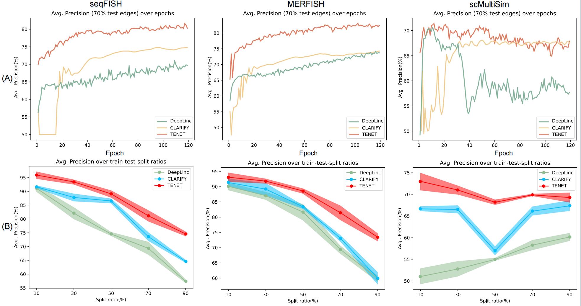
Figure 5. Model performance comparison. A. Experiment conducted on three datasets under the segmentation of 70% (TENET in red, CLARIFY in yellow, and DeepLinc in green). B. The shadow in the shadow plot with the upper and lower boundaries extends to the maximum and minimum values of the AP results. DeepLinc in green, CLARIFY in blue, and TENET in red. Results are obtained from three repeated experiments.
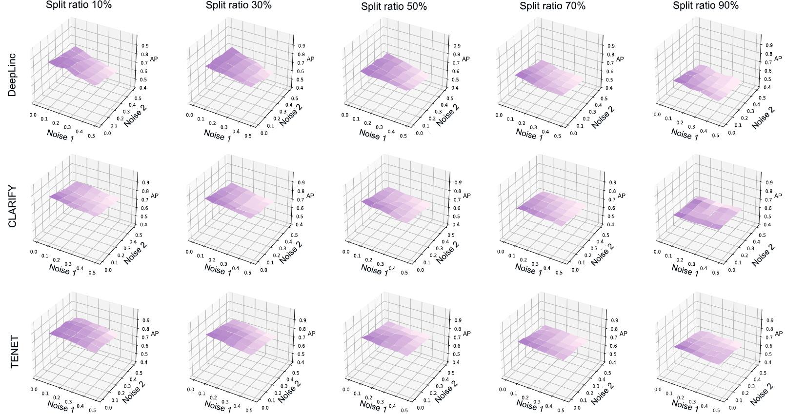
Figure 6. Experiment conducted on three of the models using the dataset of seqFISH aiming to evaluate the model's tolerance to noise (Noise1 and Noise2). At each train-test-split ratio, the ratio of Noise1 and Noise2 gradually increases from 0 to 0.5 steps with a size of 0.1. The result in each subgraph is the average of three independent experiments under the condition of 120 epochs execution.
B. Tolerance to noisy data
The tolerance to noisy data experiment is designed to simulate poor data quality, including error-detection issues and missing or incorrectly detected edges in the experimental setup. In Noise1 experiment, a certain percentage of false edges are intentionally added to Gc and Gg. In Noise2 experiment, the existing edges are removed in proportion. We aim to mimic these scenarios and assess the model's ability to handle such challenges. These experiments are conducted under the condition of train-test-split ratios of 10%, 30%, 50%, 70%, and 90% on the dataset of seqFISH. The proportion of Noise1 and Noise2 increases from 0.0 to 0.5 with steps of 0.1, resulting in 36 AP values in each subplot in Figure 6. The values outside the bracket in Table 2 can represent the stability of the model with the increment of noise (Noise1 and Noise2) ratios. The value outside the bracket on one train-test-split ratio represents the elevation difference between Value1 (Noise1 and Noise2 = 0.0) and Value2 (Noise1 and Noise2 = 0.5). The value inside the bracket at one train-test-split ratio represents the average value of 36 AP, used to facilitate comparison among models.
Table 2. AP elevation difference of Noise1, Noise2 = 0.0, and (Noise1 and Noise2 = 0.5 on the same train-test-split ratio. The value in the bracket is the average AP from all proportions of the two noises on the same train-test-split ratio (36 AP values on one train-test-split ratio).
AP elevation difference | Train-test-split ratio | |||||
| 10 | 30 | 50 | 70 | 90 | ||
| Model | ||||||
| DeepLinc | 30.22 (77.39) | 26.91 (74.01) | 23.74 (66.21) | 22.09 (57.86) | 17.27 (49.83) | |
| CLARIFY | 17.20 (83.86) | 19.12 (81.04) | 18.33 (75.13) | 10.13 (69.22) | 6.75 (61.64) | |
| TENET | 16.25 (88.89) | 16.73 (85.37) | 12.73(82.17) | 12.12 (75.39) | 7.02 (67.58) | |
* The best result for each model on each split ratio is highlighted in bold, and the second-best result is underlined.
General notes and troubleshooting
General notes
In Figure 7, there are two approaches to setting up the TENET environment. The simplest method is to utilize the provided environment.yml file (A); however, some dependencies may not be easily installed. Therefore, the recommended approach is the second way (B). Initially, create a Python virtual environment, then activate it and start installing the packages using the requirement.txt file. This file contains packages that can be downloaded without significant difficulty. Before installing the remaining packages, verify the CUDA version you are employing. If the CUDA version differs from this, the corresponding URL should be modified accordingly.
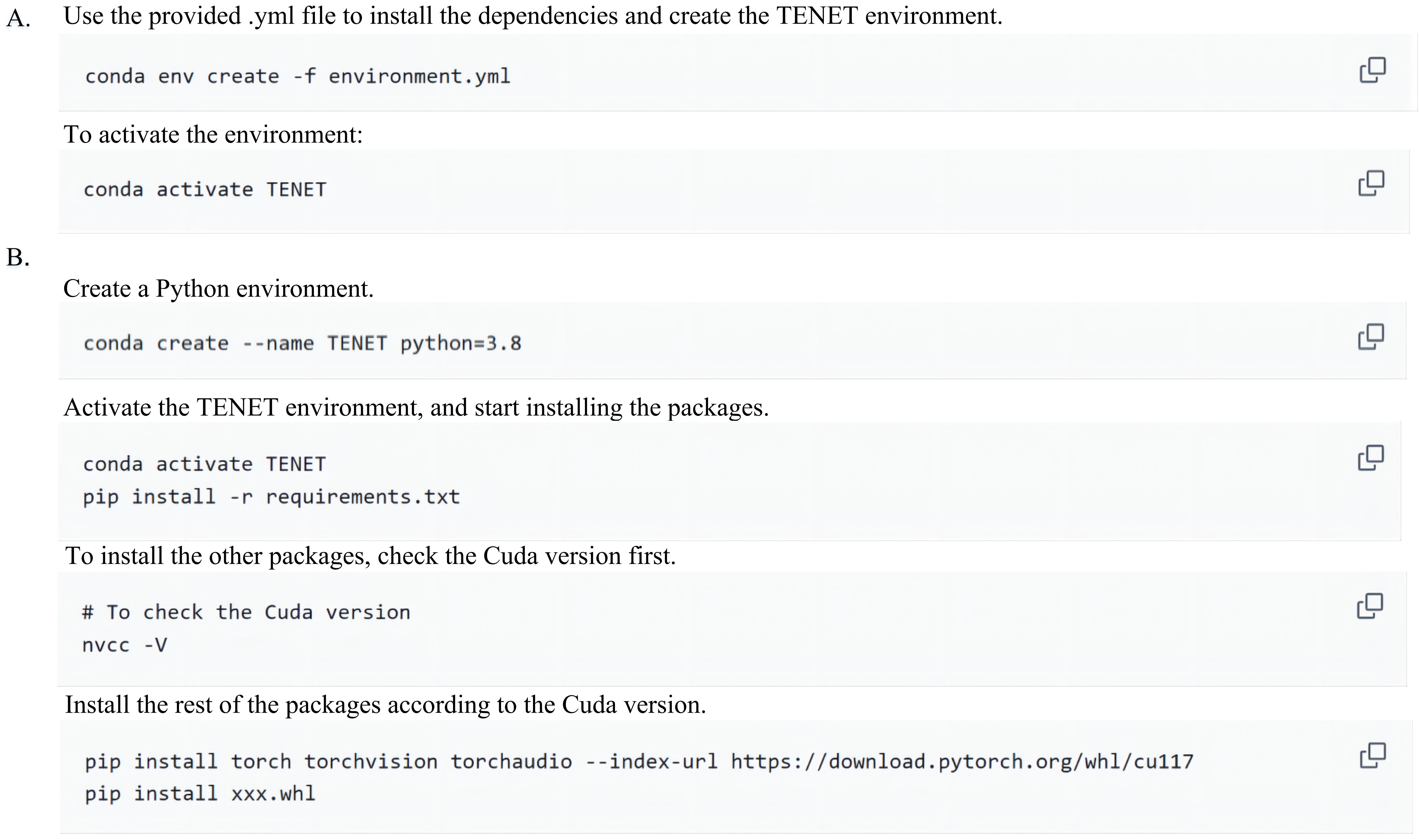
Figure 7. Environment preparation
To start training the model, use cd TENET to enter the program directory and use python main.py. The hyper-parameters can be adjusted according to the actual demand. The explanations of hyper-parameters in Figure 8 are as follows:
-m: "preprocess", this mode will construct the cell-level graph and gene-level graph using the provided method. This is necessary to generate the required graph structures before training the model. "train" this mode assumes that the cell-level graph and gene-level graph have already been constructed. It will use the provided graph structures to start the CCI reconstruction process.
-i: the input data frame path.
-o: the output results' path.
-t: train-test split ratio, the value ranges from 0 to 1. If default = 0.7, the test edges account for 70% percent of all.
-n, -k: these two hyper-parameters will be used when the mode (-m) is set to be "preprocess, where -n specifies the number of selected genes to be used when constructing the gene-level graph within each cell, -k controls the number of proximal interaction cells to be used.
-fp, -fn: the two noise ratios, their values range from 0 to 1. Introducing artificial noise to the constructed cell level graph can examine the model's tolerance to noises.
-lr: the value of the learning rate.
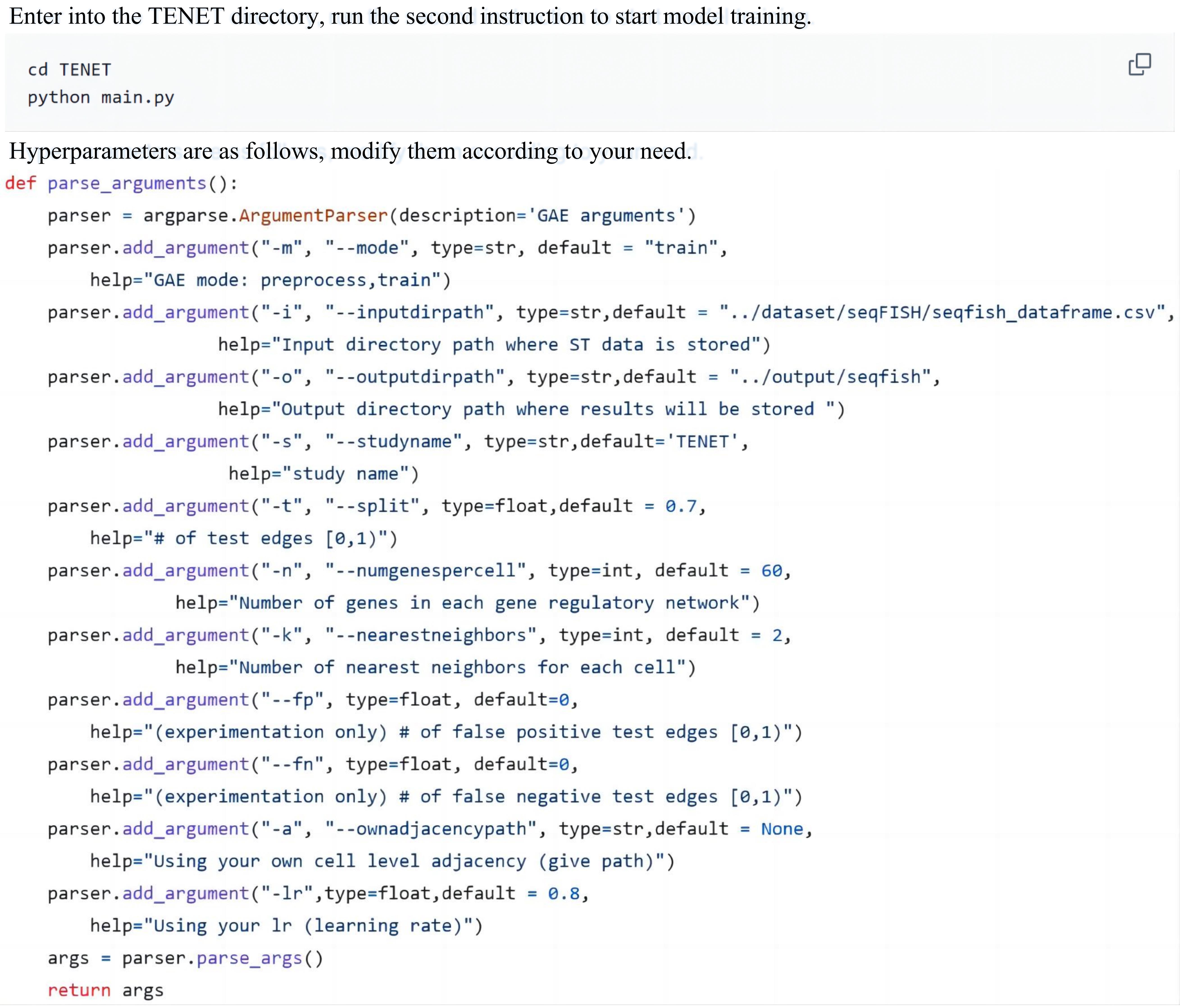
Figure 8. Hyper-parameters settings
Troubleshooting
The PyTorch version in TENET is 2.0.1 and the CUDA version is 11.7.
When installing PyTorch-related dependencies (torch-cluster, torch-scatter, torch-sparse, torch-spline-conv, and torch-geometric), they can be challenging to install and may require extended installation times. The recommendation is to download the respective .whl file via https://pytorch-geometric.com/whl (ensure you check the PyTorch version and CUDA version) and proceed with the installation.
Acknowledgments
This work is supported by the Guangdong Provincial Department of Education (2022KTSCX152), the Key Laboratory IRADS, Guangdong Province (2022B1212010006, R040000122), Guangdong Higher Education Upgrading Plan (2021-2025) with UIC Research Grant UICR0400025-21. The icons of the graphical abstract are created from https://BioRender.com.
Competing interests
The authors declare no conflicts of interest.
References
- Schwager, S. C., Taufalele, P. V. and Reinhart-King, C. A. (2018). Cell–Cell Mechanical Communication in Cancer. Cell Mol Bioeng. 12(1): 1–14. https://doi.org/10.1007/s12195-018-00564-x
- Dries, R., Zhu, Q., Dong, R., Eng, C. H., Li, H., Liu, K., Fu, Y., Zhao, T., Sarkar, A., Bao, F., et al. (2021). Giotto: a toolbox for integrative analysis and visualization of spatial expression data. Genome Biol. 22(1): 1–31. https://doi.org/10.1186/s13059-021-02286-2
- Tanevski, J., Flores, R. O. R., Gabor, A., Schapiro, D. and Saez-Rodriguez, J. (2022). Explainable multiview framework for dissecting spatial relationships from highly multiplexed data. Genome Biol. 23(1): 1–31. https://doi.org/10.1186/s13059-022-02663-5
- Li, R. and Yang, X. (2022). De novo reconstruction of cell interaction landscapes from single-cell spatial transcriptome data with DeepLinc. Genome Biol. 23(1): 1–24. https://doi.org/10.1186/s13059-022-02692-0
- Scarselli, F., Gori, M., Tsoi, A. C., Hagenbuchner, M. and Monfardini, G. (2008). The Graph Neural Network Model. IEEE Transactions on Neural Networks. 20(1): 61–80. https://ieeexplore.ieee.org/document/4700287
- Peterson, L. E. (2009). K-nearest neighbor. Scholarpedia, 4(2):1883.
- Bafna, M., Li, H. and Zhang, X. (2023). CLARIFY: cell–cell interaction and gene regulatory network refinement from spatially resolved transcriptomics. Bioinformatics 39: i484–i493. https://doi.org/10.1093/bioinformatics/btad269
- Kipf, T. N. and Welling, M (2016). Semi-supervised classification with graph convolutional networks. arXiv preprint arXiv:1609.02907 https://doi.org/10.48550/arXiv.1609.02907
- Li, H., Zhang, Z., Squires, M., Chen, X., Zhang, X. (2023). scMultiSim: simulation of multi-modality single cell data guided by cell-cell interactions and gene regulatory networks. Res Sq. 15: rs.3.rs-2675530. https://doi.org/10.21203/rs.3.rs-2675530/v1
- Zhang, X., Niu, X., Fournier-Viger, P. and Wang, B. (2022). Two-Stage Traffic Clustering Based on HNSW. Lect Notes Comput Sci. 609–620. https://doi.org/10.1007/978-3-031-08530-7_51
- Zhang, J., Fei, J., Song, X. and Feng, J. (2021). An Improved Louvain Algorithm for Community Detection. Math Probl Eng. 2021: 1–14. https://doi.org/10.1155/2021/1485592
- Cang, Z., Zhao, Y., Almet, A. A., Stabell, A., Ramos, R., Plikus, M. V., Atwood, S. X. and Nie, Q. (2023). Screening cell–cell communication in spatial transcriptomics via collective optimal transport. Nat Methods. 20(2): 218–228. https://doi.org/10.1038/s41592-022-01728-4
- McCoy-Simandle, K., Hanna, S. J. and Cox, D. (2016). Exosomes and nanotubes: Control of immune cell communication. Int J Biochem Cell Biol. 71: 44–54. https://doi.org/10.1016/j.biocel.2015.12.006
- Shao, X., Li, C., Yang, H., Lu, X., Liao, J., Qian, J., Wang, K., Cheng, J., Yang, P., Chen, H., et al. (2022). Knowledge-graph-based cell-cell communication inference for spatially resolved transcriptomic data with SpaTalk. Nat Commun. 13(1): 4429. https://doi.org/10.1038/s41467-022-32111-8
- Zhang, Z., Han, J., Song, L. and Zhang, X. (2022). CeSpGRN: Inferring cell-specific gene regulatory networks from single cell multi-omics and spatial data. bioRxiv : e482887. https://doi.org/10.1101/2022.03.03.482887
- Grover.A. and Leskovec, J. (2016). node2vec: Scalable feature learning for networks. In Proceedings of the 22nd ACM SIGKDD international conference on Knowledge discovery and data mining, pages 855–864.
- Zhong, Z., Li, C. T. and Pang, J. (2022). Personalised meta-path generation for heterogeneous graph neural networks. Data Min Knowl Discovery. 36(6): 2299–2333. https://doi.org/10.1007/s10618-022-00862-z
- Zhang, J. and Zhu, Y. (2021). Meta-path Guided Heterogeneous Graph Neural Network For Dish Recommendation System. J Phys Conf Ser. 1883(1): 012102. https://doi.org/10.1088/1742-6596/1883/1/012102
- Zhang, Y., Yan, Y., Li, J. and Wang, H. (2023). Mrcn: A novel modality restitution and compensation network for visible-infrared person re-identification. arXiv. 2303.14626. https://doi.org/10.48550/arXiv.2303.14626
- Veličković, P., Cucurull, G., Casanova, A., Romero, A., Lio, P. and Bengio, Y. (2017). Graph attention networks. arXiv preprint arXiv:1710.10903, 2017. https://doi.org/10.48550/arXiv.1710.10903
- Hu, J., Shen, L. and Sun, G. (2018). Squeeze-and-excitation networks. In Proceedings of the IEEE conference on computer vision and pattern recognition. 7132–7141. https://ieeexplore.ieee.org/document/8578843
- Kipf, T. N. and Welling, M. (2016). Variational graph auto-encoders. arXiv: 1611.07308. https://doi.org/10.48550/arXiv.1611.07308
- Ruby, U. and Yendapalli, V. (2020). Binary cross entropy with deep learning technique for image classification. Int J Adv Trends Comput Sci Eng. 9(10). http://dx.doi.org/10.30534/ijatcse/2020/175942020
- Nguyen, H. V. and Bai, L. (2011). Cosine Similarity Metric Learning for Face Verification. Lect Notes Comput Sci : 709–720. https://doi.org/10.1007/978-3-642-19309-5_55
- Sohn, K. (2016). Improved deep metric learning with multi-class n-pair loss objective. Adv Neural Inf Process Syst. 29: 1857–1865.
Article Information
Publication history
Received: Jul 18, 2024
Accepted: Dec 25, 2024
Available online: Jan 21, 2025
Published: Feb 5, 2025
Copyright
© 2025 The Author(s); This is an open access article under the CC BY-NC license (https://creativecommons.org/licenses/by-nc/4.0/).
How to cite
Wang, Z., Lee, Y., Xu, Y., Gao, P., Yu, C. and Chen, J. (2025). Model Architecture Analysis and Implementation of TENET for Cell–Cell Interaction Network Reconstruction Using Spatial Transcriptomics Data. Bio-protocol 15(3): e5205. DOI: 10.21769/BioProtoc.5205.
Category
Bioinformatics and Computational Biology
Systems Biology > Spatial transcriptomics
Molecular Biology > RNA > RNA localisation
Do you have any questions about this protocol?
Post your question to gather feedback from the community. We will also invite the authors of this article to respond.