- Protocols

- Articles and Issues
- For Authors
- About
- Become a Reviewer

Utilizing FRET-based Biosensors to Measure Cellular Phosphate Levels in Mycorrhizal Roots of Brachypodium distachyon
Published: Vol 15, Iss 2, Jan 20, 2025 DOI: 10.21769/BioProtoc.5158 Views: 2389
Reviewed by: Demosthenis ChronisJuliane K IshidaAnonymous reviewer(s)
Original research article
The authors used this protocol in:
Jun 2022
Advertisement


Protocol Collections
Comprehensive collections of detailed, peer-reviewed protocols focusing on specific topics


Abstract
Arbuscular mycorrhizal (AM) fungi engage in symbiotic relationships with plants, influencing their phosphate (Pi) uptake pathways, metabolism, and root cell physiology. Despite the significant role of Pi, its distribution and response dynamics in mycorrhizal roots remain largely unexplored. While traditional techniques for Pi measurement have shed some light on this, real-time cellular-level monitoring has been a challenge. With the evolution of quantitative imaging with confocal microscopy, particularly the use of genetically encoded fluorescent sensors, live imaging of intracellular Pi concentrations is now achievable. Among these sensors, fluorescence resonance energy transfer (FRET)-based biosensors stand out for their accuracy. In this study, we employ the Pi-specific biosensor (cpFLIPPi-5.3m) targeted to the cytosol or plastids of Brachypodium distachyon plants, enabling us to monitor intracellular Pi dynamics during AM symbiosis. A complementary control sensor, cpFLIPPi-Null, is introduced to monitor non-Pi-specific changes. Leveraging a semi-automated ImageJ macro for sensitized FRET analysis, this method provides a precise and efficient way to determine relative intracellular Pi levels at the level of individual cells or organelles.
Key features
• This protocol describes the use of FRET biosensors for in vivo visualization of spatiotemporal phosphate levels with cellular and subcellular resolution in Brachypodium distachyon.
• An optimized growth system can allow tracing of Pi transfer between AM fungi and host root.
Keywords: ArbusculesBackground
Arbuscular mycorrhizal (AM) fungi establish one of the most prevalent mutualistic relationships with plants, primarily delivering phosphorus in the form of phosphate (Pi) to their hosts for carbon in return. The symbiosis is characterized by AM fungal hyphae penetrating the root epidermis, progressing through the root to the cortex, and forming arbuscules within cortical cells. The arbuscules, intricate tree-like structures, serve as the primary sites for nutrient exchange.
Mycorrhizal roots contain a diverse array of cortical cell conditions including cells hosting intracellular hyphae and cells containing arbuscules at different stages of development, from initiation to maturity and eventual collapse [1,2]. This diversity in arbuscule development across the cortical cells is predicted to result in variation in Pi transfer, as periarbuscular membrane-resident Pi transporters show arbuscule stage–specific expression [3–6]. Therefore, variance in Pi content in these cells is anticipated. In addition, plastids in certain colonized cells become highly stromulated [7,8], suggesting increased metabolic activity that may result in intracellular shifts in Pi levels.
Furthermore, the process of Pi uptake in mycorrhizal roots markedly contrasts with that of non-mycorrhizal roots. While non-mycorrhizal roots absorb Pi through their epidermal cells, transporting it apoplastically and/or sequentially to the cortex, endodermis, and vasculature, mycorrhizal roots receive Pi uptake directly into their inner cortical cells before moving it to the endodermis and vasculature [5,6]. Epidermal Pi transporter gene expression is downregulated in mycorrhizal roots, suggesting that the epidermis in mycorrhizal roots plays a less significant role in Pi absorption [9–11]. Given these distinct pathways for Pi uptake, investigating the cellular Pi response dynamics within mycorrhizal roots is likely to provide new insights into root Pi distribution and homeostasis.
Genetically encoded fluorescent sensors have emerged as powerful tools for monitoring analytes with cellular resolution [12,13]. These fluorescent sensors can be introduced into plants and expressed from constitutive or tissue/cell-type-specific promoters. They have the ability to bind reversibly to their analytes, translating their abundance into fluorescence changes. This facilitates real-time monitoring of molecular changes at intracellular or subcellular levels. Biosensors, targeting ions like Ca2+, H+, and Zn2+, as well as hormones such as ABA and auxin, and monitoring protein activities such as nitrate transporters, have been created and used in plants [12]. Their application has advanced knowledge of ion and hormone dynamics during plant development and in response to abiotic stress [13–15].
Among the various biosensors, fluorescence resonance energy transfer (FRET)-based sensors have proven especially reliable [12,13]. FRET occurs when a donor and an acceptor fluorescent molecule are in close proximity, and there is spectral overlap between the donor emission and the acceptor excitation; energy then transfers from the excited donor to the acceptor, quenching the donor’s fluorescence and potentially enhancing fluorescence of the acceptor. FRET biosensors generally feature a ligand-binding domain attached to two green fluorescent protein (GFP) spectral variants, typically cyan (CFP) and yellow (YFP). When the ligand binds, it triggers a conformational change that alters the proximity of the donor and acceptor and affects the FRET efficiency. This change is observed as a shift in the intensity ratio of the two fluorescent proteins, termed the FRET ratio [13]. The observed ratio directly corresponds to the ligand concentration within a range defined by the binding affinity and, ultimately, by the sensor's saturation point [16–18]. Furthermore, FRET-sensitized emission is a valuable method to measure FRET; adjusting for issues like donor spectral bleed-through and acceptor cross-excitation allows a precise determination of FRET-derived acceptor fluorescence [19–21]. Such adjustments are vital when analyzing ligand concentrations across various cell types or comparing data from different samples to pinpoint gene or protein roles.
To measure Pi content in mycorrhizal roots, we introduced a Pi biosensor, cpFLIPPi-5.3m, into Brachypodium distachyon plants and targeted it to the cytosol or plastid [22]. In each case, we included a control sensor, cpFLIPPi-Null, which has a mutation that prevents Pi binding. These sensors had previously been optimized and used successfully to monitor intracellular Pi content in Arabidopsis thaliana [23,24]. The authors had shown that the control sensor is Pi-independent and any FRET ratio shifts reflect non-Pi specific changes, such as intracellular ionic shifts. Thus, when the control sensor exhibits no FRET ratio shift, it suggests that the observed changes in the Pi sensor are genuinely due to intracellular Pi fluctuations. This study outlines our method of employing these sensors to track Pi dynamics during AM symbiosis and our use of a semi-automated ImageJ macro to efficiently extract quantitative data for sensitized FRET analysis.
Materials and reagents
Biological materials
1. All Brachypodium distachyon (line Bd21-3) transgenic lines used in this protocol can be obtained from Maria Harrison’s lab (under a Boyce Thompson Institute Material Transfer Agreement). The lines are grouped into categories as follows:
a. For the quantification of cytosolic Pi levels:
Transgenic lines expressing the sensor and its controls from a mycorrhiza-inducible, cell-type-specific promoter, BdPT7. Fluorescent signals from these lines are only from cells containing arbuscules.
BdPT7::cpFLIPPi-5.3m
BdPT7::cpFLIPPi-Null
BdPT7::eCFP
BdPT7::cpVenus
WT (used as a negative control to remove the potential background during image analysis)
All lines are needed for Pi imaging for each experiment.
Transgenic lines expressing the sensor and controls from the constitutive promoter ZmUb1 promoter. Fluorescent signals from these lines occur in all cell types. We failed to generate a ZmUb1::cpVenus line so the BdPT7::cpVenus is used as one of the controls for ZmUb1::cpFLIPPi-5.3m.
ZmUb1::cpFLIPPi-5.3m
ZmUb1::cpFLIPPi-Null
ZmUb1::eCFP
BdPT7::cpVenus
WT (used as a negative control to remove the potential background during image analysis)
b. For the quantification of plastidic Pi levels:
Transgenic lines expressing a plastid-targeted sensor and its controls from the BdPT7 promoter. Fluorescent signals from these lines occur in the plastid only in cells containing arbuscules.
BdPT7::plastid-cpFLIPPi-5.3m
BdPT7::plastid-cpFLIPPi-Null
BdPT7::plastid-eCFP
BdPT7::plastid-cpVenus
WT (used as a negative control to remove the potential background during image analysis)
2. AM fungal spores. Diversispora epigaea is used in the protocol as an example. It can be obtained from the International Collection of (Vesicular) Arbuscular Mycorrhizal Fungi (INVAM). Other species of AM fungi are also available from this collection. We have also used these lines successfully with Rhizophagus irregularis. A commercial vendor, Premier Tech (Canada), can supply Rhizophagus irregularis (ready-for-use spores).
Reagents
1. Bleach (Pure Bright, containing 5%–7% sodium hypochlorite)
2. Sterile deionized water
3. Agar (Millipore-Sigma, catalog number: A7921)
4. Benomyl [Methyl 1-(butylcarbamoyl)-2-benzimidazolecarbamate] (Millipore-Sigma, catalog number: 381586)
5. Ca(NO3)2·4H2O (calcium nitrate tetrahydrate) (Millipore-Sigma, catalog number: C2786-500G)
6. KNO3 (potassium nitrate) (Millipore-Sigma, catalog number: 221295-100G)
7. MgSO4·7H2O (magnesium sulfate heptahydrate) (Millipore-Sigma, catalog number: 221295-100G)
8. NaFeEDTA [ethylenediaminetetraacetic acid iron(III) sodium salt] (Millipore-Sigma, catalog number: EDFS-100G)
9. KH2PO4 (potassium phosphate monobasic) (Millipore-Sigma, catalog number: P0662-25G)
10. H3BO3 (boric acid) (Millipore-Sigma, catalog number: B0394-100G)
11. Na2MoO4·2H2O (sodium molybdate dihydrate) (Millipore-Sigma, catalog number: 331058-5G)
12. ZnSO4·7H2O (zinc sulfate heptahydrate) (Millipore-Sigma, catalog number: 221376-100G)
13. MnCl2·4H2O [manganese(II) chloride tetrahydrate] (Millipore-Sigma, catalog number: 221279-100G)
14. CuSO4·5H2O [copper(II) sulfate pentahydrate] (Millipore-Sigma, catalog number: 209198-5G)
15. CoCl2·6H2O [cobalt(II) chloride hexahydrate] (Millipore-Sigma, catalog number: 255599-5G)
16. HCl (hydrochloric acid) (Millipore-Sigma, catalog number: 258148-25ML)
17. MES (C6H13NO4S) (Millipore-Sigma, catalog number: M3671-50G)
18. NaOH (sodium hydroxide) (Millipore-Sigma, catalog number: 221465-500G)
Solutions
1. Modified 1/4 strength Hoagland solution with 20 μM potassium phosphate (see Recipes)
Recipes
1. Modified 1/4 strength Hoagland solution with 20 μM potassium phosphate
| Reagent | Final concentration | Note |
|---|---|---|
| Ca(NO3)2·4H2O | 1.25 mM | |
| KNO3 | 1.25 mM | |
| MgSO4·7H2O | 0.5 mM | |
| NaFeEDTA | 0.025 mM | |
| KH2PO4 | 0.02 mM | The phosphate levels can be varied by adjusting the amount of this reagent. |
| H3BO3 | 5 μM | |
| Na2MoO4·2H2O | 0.12 μM | |
| ZnSO4·7H2O | 0.5 μM | |
| MnCl2·4H2O | 1 μM | |
| CuSO4·5H2O | 0.25 μM | |
| CoCl2·6H2O | 0.19 μM | |
| HCl | 6.25 μM | |
| MES (C6H13NO4S) | 0.25 mM |
Adjust the final pH to 6.1 using NaOH.
Laboratory supplies
1. 14 mL culture polypropylene tubes (MTC-Bio, catalog number: UX-34501-06)
2. Regular-weight seed germination paper (Anchor Paper Co, catalog number: SD3815L)
3. Sterile Petri dish (100 × 10, Carolina, catalog number: 741248; 100 × 20 mm, Carolina, catalog number: 741252; a large one, approximately 14 cm in diameter, used for washing substrate from roots)
4. Parafilm (Sigma-Aldrich, catalog number: P7543)
5. 20 cm plastic cones (Stuewe & Sons, Inc., catalog number: SC10U)
6. 9 cm (3-1/2”) diameter plastic pot (Flinn Scientific, catalog number: FB0652)
7. Humidity domes (Global Industrial, catalog number: CK64081)
8. Growth substrate (for example, sand, gravel, or turface, which can be purchased from a general supplier, e.g., Lowes or Home Depot)
9. MF Millipore membrane filter, 0.45 μm pore size (Millipore-Sigma, catalog number: HAWP9000)
10. Microscope slides (ideally 75 mm × 25 mm, Carolina, catalog number: 632010) and coverslips (ideally 20 mm × 20 mm, Carolina, catalog number: 633009)
11. Aluminum foil
12. Fine tip tweezers (Fisherbrand, catalog number: 12-000-122)
13. A digital camera or other device that can take photos, such as a personal cell phone
14. Spray bottles (UNLINE, catalog number: S-11686)
Equipment
1. Class I laminar flow hood (e.g., Thermo Scientific HeraguardTM ECO Clean Bench, catalog number: 51029701)
2. Growth chambers or greenhouses to grow plants (e.g., Conviron reach-in growth chamber, model: PGR15)
3. Stereomicroscope (Olympus, model: SZX-12)
4. Upright confocal microscope (Leica, model: SP5), see General note 1 for details
Software and datasets
1. Fiji (ImageJ, free, no license needed, can be downloaded via the link: https://imagej.net/downloads)
The sensitized FRET analysis Macro can be copied via the link: https://nph.onlinelibrary.wiley.com/action/downloadSupplement?doi=10.1111%2Fnph.18081&file=nph18081-sup-0001-SupInfo.pdf)
Procedure
A. Plant material preparation
1. AM fungal spore preparation (optional if inoculating with AM fungi)
The preparation of AM fungal spores varies among fungal species and research purposes. If you have an established method, follow it. Otherwise, consider these options:
a. Obtain ready-for-use spores from the International Collection of (Vesicular) Arbuscular Mycorrhizal Fungi (INVAM) or commercial vendors like Premier Tech, Canada.
b. Refer to spore preparation methods in [26] or [27].
c. In cases when specific fungal species are not required, directly inoculate plants with commercial or home-made mixed propagule inoculum as described in these studies [28,29].
2. Seed sterilization and plant preparation [30].
Critical: For a complete Pi imaging session, prepare B. distachyon plants expressing the Pi sensor and four controls simultaneously in the same manner.
a. Place up to 50 B. distachyon seeds of the same genotype in 14 mL culture tubes.
b. Add 10 mL of 20% bleach (v/v) and shake vigorously by hand for 7 min.
c. (Under the laminar hood) Decant the bleach and rinse the seeds with sterile deionized water five times.
d. Place a sterile germination paper disc in a Petri dish, wet it with sterile deionized water, and place seeds on it (seed embryo facing paper).
e. Wrap the Petri dish with Parafilm and aluminum foil and store the seeds in the dark at 4 °C for 1 week.
f. After 1 week, move the Petri dish to room temperature for 2 days to stimulate root growth, but leave the seeds in the dark (Petri dish covered with foil is suitable).
g. Take the plates out of the dark (remove foil) and place them under light (12:12 h light/dark) for 3–5 days. The light intensity in our chamber was 150 μmol/m2·s. Then, open the plates to harden the seedlings.
The B. distachyon seedlings, with a shoot length of approximately 7 cm and a root length of about 5 cm, are now ready for planting and inoculation.
3. AM fungal inoculation setup
There are many ways to grow and inoculate B. distachyon plants; here, two types of growth systems are used for the biosensor-based analysis of intracellular Pi in mycorrhizal roots:
Preparation of growth system 1: plants in cylinder cones or pots
Fill 20 cm long plastic cones or 9 cm diameter pots with growth substrates. For the cone, fill to 5 cm below the top of the cones. For the 9 cm diameter pots, fill the substrate roughly up to half the height of the pot.
Note: Choose a suitable growth substrate that allows easy access to clean roots and nutrient management. Substrates or a mixture of substrates such as sand, gravel, and/or turface with particle sizes varying from 0.05 to 0.7 mm are recommended. Avoid vermiculite and perlite as these substrates stick to the surface of the roots, which disturbs imaging. We use gravel and yellow sand in an approximately 1:1 ratio.
a. Place the AM fungal spores or the mixed propagule inoculum mixture onto the substrate and then fill the cones or the pots with the same substrate.
b. Transplant the B. distachyon seedlings into the substrate. Cover the cones/pots with a plastic dome cover for humidity control (Figure 1).
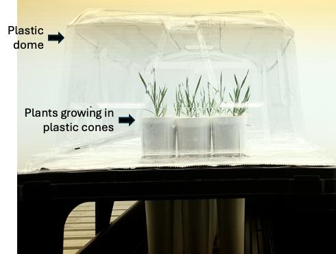
Figure 1. Demonstration of the growth system 1
c. Place the plants in a growth chamber or a greenhouse under a 12:12 h, 24:22 °C light/dark cycle. The light intensity in our chamber was 150 μmol/m2·s. Grow plants for four weeks watering with deionized water as needed. Fertilize once per week with 10 mL of 1/4 strength modified Hoagland solution containing 20 μM potassium phosphate (or as needed depending on the growth substrate used).
Note: High Pi levels in the fertilizer may inhibit fungal colonization of the host roots.
d. One day before imaging, provide plants with 10 mL of 1/4 strength modified Hoagland solution supplemented with 2 μM potassium phosphate (generating a lower Pi environment).
Preparation of growth system 2: plants inoculated between cellulose membranes
a. Sandwich a seedling and some fungal spores between two pieces of MF Millipore membrane filter discs. Position the spores around the root (Figure 2A).
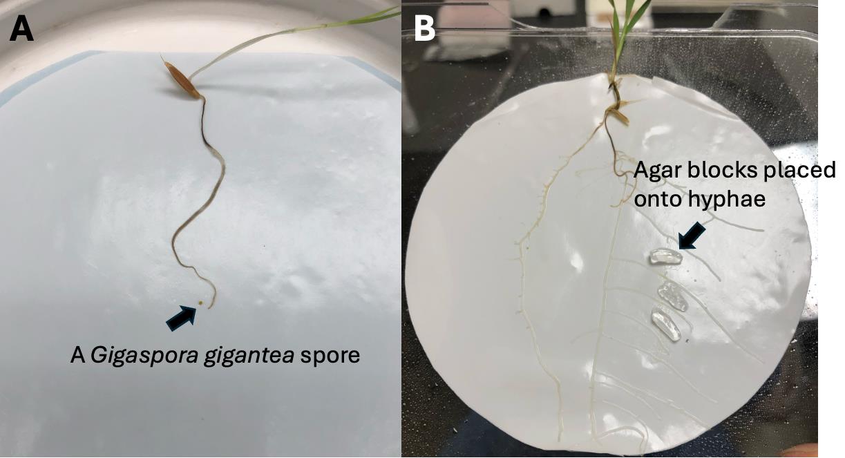
Figure 2. Demonstration of the growth system 2. A. A Gigaspora gigantea spore placed next to the seedling during the system setup. B. Agar blocks placed onto the fungal hyphae to start localized treatment.
b. Place the sandwich with plants and spores vertically in the earlier discussed sand/gravel mix in a 9 cm diameter pot.
c. Set the plants in the same growth condition as described in step c in the section “Preparation of growth system 1”.
B. Preparation of B. distachyon roots for Pi imaging
Note: This procedure is tailored for Pi imaging using an upright microscope. If an inverted microscope is used, adjustments will be needed.
Growth system 1
1. Carefully remove the plants from the cones and place the root in a large Petri dish (14 cm diameter).
2. Rinse the roots gently with running water to remove substrates.
3. Immerse the roots in the container with 1/4× modified Hoagland solution with 2 μM potassium phosphate (the same Pi concentration as the final fertilizer treatment as reported in step d in the section “Preparation of growth system 1”).
Critical: To minimize the intracellular Pi disturbance due to manipulation, ensure the Pi concentration in the container matches the solution last used to maintain the plants unless another treatment is required.
4. Use a fluorescence stereomicroscope to locate a colonized root.
Note: While checking the root under the microscope, use tweezers to isolate a single root branch and gently slide it onto the glass slide.
5. Transfer the root region to the center of a microscope slide (ideally 75 mm × 25 mm). Cover it with a coverslip (ideally 20 mm × 20 mm) to maintain stability and flatness during imaging (Figure 3). If necessary, add a few drops of the 1/4 modified Hoagland solution with 2 μM potassium phosphate on the side of the coverslip.
Note: If AM fungal colonization is not required, omit steps B4 and B5, directly place a root region of interest onto the microscope slide, and cover it with a coverslip as described.
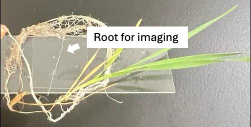
Figure 3. Arrangement of the root on the glass slide for confocal imaging
6. Gather the rest of the attached root and shoot around the edge of the coverslip (some may hang outside the slide).
7. Frequently spray the root and shoot with 1/4 modified Hoagland solution with 2 μM potassium phosphate to maintain moisture.
Growth system 2
This growth system allows a local application of Pi or chemical treatment directly to mycorrhizal roots or their connected extraradical hyphae of the fungi. The treatment is applied via solid agar blocks. Below is an example of using the system to provide a local Pi treatment of 200 μM Pi.
1. Prepare a 1/4× modified Hoagland solution containing 200 μM Pi and 1% (w/v) agar immediately before the experiment. Agar is dissolved by heating in a microwave.
Note: Sterile Hoagland solution is recommended to avoid contamination.
2. Pipette the solution into a Petri dish in 10 μL droplets and allow them to solidify.
3. Gently remove the MF Millipore membrane with the plant from the pots and place it in a ~20 cm diameter flat-bottomed container.
4. Carefully remove one MF Millipore membrane and expose the roots and fungus. Gently remove the substrates on the membrane.
Critical: Some roots grow into or through the MF Millipore membrane. Make sure the removal process does not break the roots.
5. Locate the colonized root regions and their connecting fungal hyphae. If using non-colonized roots, locate and mark the root regions of interest. Mark the site for applying the agar blocks and take photographs with distance scales for reference.
6. Place the solidified agar blocks over the roots or the extraradical hyphae at the marked sites (Figure 2B). If incubation is needed, place the membrane with the plant inside a closed container, ensuring that the shoot remains outside of the container. For example, use a 14 cm Petri dish with one side removed. The shoot can be left outside. Periodically spray the membrane with 1/4 modified solution without Pi to maintain a moist environment. The system can be left in the dark or light as needed. When applying a localized treatment to the extraradical hyphae, it may be useful to have a Benomyl-treated control. Benomyl is a fungicide, and fungal activity can be abolished by applying 1 mL of 100 μg/μL Benomyl to the mycorrhizal root system one day before the experiment (as used in [22]). This Benomyl-treated control enables an assessment of diffusion along the hyphae vs. active transport by the fungus.
7. Remove the agar blocks after 24 h of incubation. If imaging is required after the treatment, transfer the membrane with the plant onto a glass slide (ideally 75 mm × 25 mm), ensuring that the marked region is at the center of the slide.
8. Place a coverslip (ideally 20 mm × 20 mm) over the region of interest on the membrane. If necessary, add a few drops of the 1/4 modified Hoagland solution without phosphate on the side of the coverslip. Frequently spray the membrane with Hoagland solution without phosphate to maintain moisture throughout the procedure.
C. Confocal imaging of roots
Critical: See General note 1 to determine how to set the confocal settings.
1. Once confocal settings are finalized, begin imaging roots expressing either the Pi or control biosensor. Each image set should include CC (CFP excitation—CFP emission), CY (CFP excitation—YFP emission), and YY (YFP excitation—YFP emission) images. For roots generated using growth system 2, position the glass slides with the membrane directly on the microscope stage. When imaging a colonized root, ensure that the images capture the targeted arbuscules and that the arbuscules are distinct.
Note: Aim for a minimum of six biological replicates (individual roots) in each treatment group to ensure robust statistical analysis. Ideally, obtain at least five clear images showcasing at least five arbuscules in the desired colonized region for each root.
Critical: To ensure integration with our FLIPPi image analysis macro in ImageJ, maintain specific image file names when saving image files.
The suggested file naming system is pPT7_cytFLIPPi_053019_HP_0.5h_102
(sensor name) (date) (group) (plant & image number)
You can adjust the name and order of components, such as the line name, date, and treatment group, as needed. However, the plant and image number “_102” format must be retained. In this format, “1” signifies the first root, while “2” indicates it is the second image of that root. For instance, for the 10th image of root 6, the plant and image number would be “_610.” This format provides a unique identifier, allowing the FLIPPi macro to distinguish individual images from each plant.
2. After imaging all samples with the Pi and control biosensors, proceed to image the roots expressing eCFP and cpVenus. Each set of images should contain all CC, CY, and YY images.
Note: At least three biological replicates are recommended for eCFP and cpVenus, capturing a minimum of five distinct images per replicate.
D. Image processing and sensitized FRET analysis
Sensitized FRET ratios eliminate non-FRET emissions such as CFP bleed-through and YFP (or cpVenus) cross-excitation. Each image requires standard processing. The sensitized FRET analysis can be conducted for each image set (CC, CY, and YY). For efficiency, utilize the FLIPPi macro, which is designed primarily for images from Leica confocal microscopes. For other confocal types, adjust file names to fit the macro as suggested in step C1. Once the folders are directed to the FLIPPi macro, it automatically processes images and calculates CC, CY, and YY values after selecting the regions of interest (ROIs) (Figure 4). Usually, up to five ROIs can be selected per image.
Note: The macro is compatible with both MacOS and Microsoft operating systems.
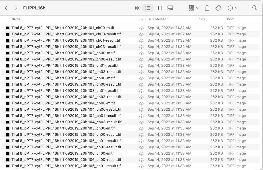
Figure 4. Screenshot showcasing a sample folder with FRET images, adhering to the suggested file naming system
1. Open Fiji, find Plugins menu, go to Macros → Startup Macro. A window (Figure 5) will show up.
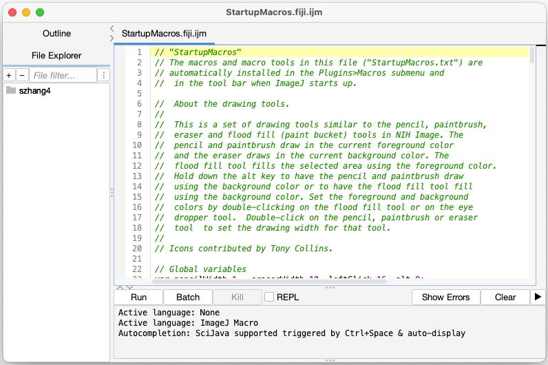
Figure 5. Screenshot showing the window following the selection of the Startup Macro option
2. Remove the green script as they are the default description from Fiji. Insert the command lines from Method S1 in [22]. Click Run. A subsequent window (Figure 6) will appear.
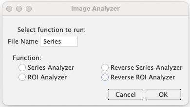
Figure 6. Screenshot showing the window following clicking Run
3. Keep the “File Name [Blank]” at its default setting. Choose one of the four functions: Series Analyzer, Reverse Series Analyzer, ROI Analyzer, or Reverse ROI Analyzer.
The functionalities of these options are detailed below:
• Series Analyzer: This function aids in background removal. It generates a mask image that captures only the root, excluding the background. This is based on the root’s profile on CC, as these images clearly depict the root profile. Subsequently, this mask is applied to the CC, CY, and YY to remove their backgrounds. The processed images are exported into the same folder as the original images.
• Reverse Series Analyzer: This operates similarly to the Series Analyzer, but with one distinction. It employs YY to create mask images instead of CC. This is specifically useful for background removal in a control set of images from cpVenus because the fluorescence intensity of CC is not high enough for mask creation.
• ROI Analyzer: After opening the processed CC created by the Series Analyzer, this function prompts users to select their regions of interest (ROIs). It then calculates the mean grey values of these ROIs from the CC, CY, and YY images. The resultant data is in tabular form, ready to be transferred into Excel.
• Reverse ROI Analyzer: Serving a similar purpose to the ROI Analyzer, this function is specifically tailored for images from the cpVenus control. It begins by opening the processed YY in lieu of the CC.
4. Begin with unprocessed images exported from the imaging software. Select Series Analyzer and click OK. This action will prompt a file directory window to appear (Figure 7).
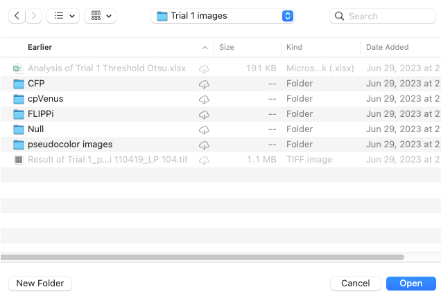
Figure 7. Screenshot showing the file directory window after step D4
Critical: Ensure that the images exported are in TIFF format. Each set of images, originating from a single ROI, should be separated into three grayscale images: CC, CY, and YY, which are categorized based on the emission collection channels. It is important that you do not use RGB format during image processing. As specified in the macro scripts (refer to Method S1 in [22]), CC is linked to channel 00 (file names conclude with “_ch00” by Leica LAS X), CY is associated with channel 01 (indicated by “_ch01”), and YY corresponds to channel 03 (“_ch03”). The macro scripts can be tailored to various naming systems.
Critical: see General note 2.
5. Select the folder that contains your original images and click Open. All images within this folder will be automatically opened, processed, and saved back to the same location.
6. Once processing is complete, navigate to the chosen folder. Transfer the processed images to the designated “processed image” folder. You can identify the processed images by their file name endings: “-m.tif” for mask images and “-result.tif” for fully processed images. Sort the files by their date modified; all processed images are placed together (Figure 8).
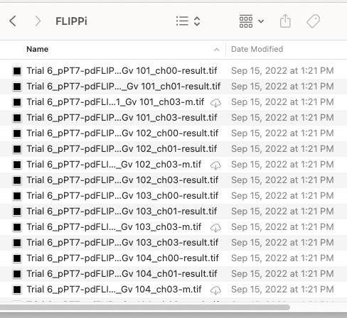
Figure 8. Screenshot showing the file directory window for step D6. Processed images end their file names with “-result.tif” or “-m.tif.”
7. Run the macro again, select ROI Analyzer, and click OK.
8. Similar to the Series Analyzer, the ROI Analyzer will sequentially open each image based on the file order in the folder. An image window will appear, accompanied by a prompt asking, “How many ROI’s would you like to use?” (Figure 9).
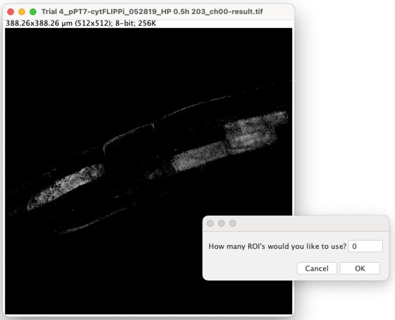
Figure 9. Screenshot showing the prompted windows for step D8
9. Depending on the number of visualized colonized cells, typically 1–5 ROIs are chosen for each image. If an image should be bypassed, enter “0” and click OK.
Note: Adjust the brightness and contrast of the images by navigating to Image → Adjust → Brightness/Contrast… This will enhance the visibility of the ROI without altering the grayscale value of each pixel.
10. Select the Oval Tool from the taskbar and begin designating oval ROIs. Each ROI should be positioned entirely within one cell. Choose an area where the signal is bright but not saturated. Once you have chosen the ROI, click OK in the pop-up Waiting window (Figure 10).
Critical: To generate accurate data, it is essential to maintain a consistent ROI size.
A Result window will appear, displaying the CC, CY, and YY values. Gather these results once the ROIs from all images in the folder have been selected.
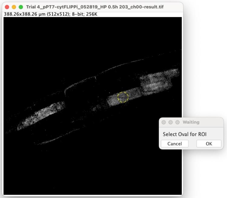
Figure 10. Screenshot showing the prompted windows for step D10
11. A subsequent Waiting window will emerge for the next ROI. Simply reposition the circle to another colonized cell in focus and continue the process. The macro will proceed to the next image once the designated number of ROIs has been selected from the current image.
Critical: Ensure that the ROI is selected prior to clicking OK. Failing to do so may cause the program to freeze, requiring a restart from the beginning.
12. Once the ROI Analyzer has completed analyzing all processed images in the folder (Figure 11), copy the results and paste them into the Excel template (refer to Table S4 in [22]). Close the Results window.
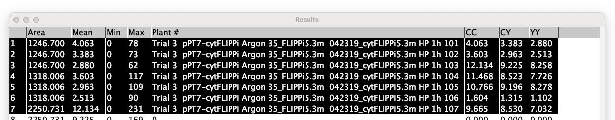
Figure 11. Screenshot showing the prompted windows for step D13
13. Continue the analysis for all the roots associated with FLIPPi, control sensors, and the eCFP control.
14. For roots associated with cpVenus, utilize the Reverse Series Analyzer and Reverse ROI Analyzer. The steps for using the Reverse Series Analyzer and Reverse ROI Analyzer mirror those of the Series Analyzer and ROI Analyzer, respectively.
15. Arrange the data within the Excel sheet template (refer to Table S4 in [22]). This template offers a structure where different treatment groups have individual tabs. Inside each tab, data are organized according to the sensor type. The columns labeled “Plant, CC, CY, and YY” are directly derived from the FIJI macro.
16. For CFP controls, transfer the columns titled “Plant,” “CC,” and “CY” to Excel. For cpVenus controls, transfer the columns “Plant,” “CY,” and “YY” to Excel.
Data analysis
Sensitized FRET represents a corrected CY value, where emissions not derived from FRET, such as CFP bleed-through and YFP (or cpVenus) cross-excitation (in both channels), are eliminated [20,21]. The equation for calculating sensitized FRET is:
Sensitized FRET = CY - CC*b - YY(c - a*b)
The coefficients a, b, and c are derived from the CFP and cpVenus controls, using ROI data and linear regression. A trendline from the linear regression illustrates the fit of each data point to the linear model (Figure 12). Specifically:
a represents the slope of CC against YY from cpVenus.
b is the slope of CY against CC from CFP.
c is the slope of CY against YY from cpVenus.
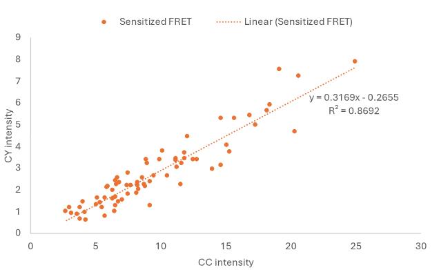
Figure 12. Example graph showing the trendline in Excel
These coefficients can be determined using Excel’s regression functions on a graph or the LINEST function [23,24,31].
Typically, the coefficient a is close to zero, allowing the calculation to be simplified to:
Sensitized FRET = CY - CC*b - YY*c
Before utilizing the simplified equation, it is important to verify the value of a. Subsequently, FRET ratios can be derived by dividing the sensitized FRET by CC. Use linear regression graphs to evaluate the linearity of the sensitized FRET. A closer alignment of data to the linear model signifies greater accuracy of the sensitized FRET result.
For a reliable and in-depth statistical assessment, it is advisable to have at least six biological replicates.
Validation of protocol
This protocol has been used and validated in the following research article:
• Zhang et al. [22]. A genetically encoded biosensor reveals spatiotemporal variation in cellular phosphate content in Brachypodium distachyon mycorrhizal roots. New Phytol 234: 1817–1831. https://doi.org/10.1111/nph.18081
General notes and troubleshooting
General notes
1. Prior to imaging, optimizing the confocal settings (such as laser, objective, filter, and scan mode) is critical for generating reliable and consistent FRET data. The goal is to obtain a high range of fluorescence intensities, but no pixels should be saturated. To achieve this goal, a few transgenic plants expressing the Pi biosensor and its three controls need to be included in the process. After the settings are confirmed, they should be kept the same across all control lines for the same Pi biosensor. If imaging tissue types and biosensor lines are changed, the optimizing process needs to be redone. The following criteria need to be considered:
• For the sensitized FRET analysis, each set of the root image from the Pi and control biosensor needs to include three images: CFP excitation—CFP emission (CC hereafter), CFP excitation—YFP emission (CY hereafter), and YFP excitation—YFP emission (YY hereafter). When capturing CC and CY, maintain the exact same confocal settings, such as the excitation wavelength and intensity, exposure time, scan speed, gain, and pinhole (if any is applicable). Ensure the fluorescent intensities of YY remain roughly equivalent to those in CC and CY.
• Because CC and CY emission collection channels are very close on the wavelength, try to narrow the two channels as much as possible to avoid bleed-through but also keep a reasonable fluorescent intensity.
• Images of non-fluorescent wildtype B. distachyon need to be included for background subtraction purposes.
• Laser power. Some lasers need warm-up time; thereby, the laser power may increase during imaging. Consider warm-up time before starting imaging.
For our experiments, the objective used for plants in growth system 1 expressing the BdPT7-cytosolic, ZmUbi-cytosolic, and BdPT7-plastidic sensors was a 63× water lens with a numerical aperture of 1.20, whereas a 20× water lens with a numerical aperture of 0.70 was used for plants growing in growth system 2. The 458 nm laser intensity (used for CC and CY) was 40% for BdPT7-cytosolic sensors, 90% for ZmUbi-cytosolic sensors, and 30% for BdPT7-plastidic sensors. The 514 nm laser intensity (used for the YY) was 10% for BdPT7-cytosolic sensors, 16% for ZmUbi-cytosolic sensors, and 7% for BdPT7-plastidic sensors. The emission ranges collected by the HyD detector for the CC channel were between 475 and 490 nm, while for the CY and YY channels, the emission range was between 546 and 562 nm. The HyD detector operated in photon counting mode for all conditions. Additional parameters included a line average of 3, a pinhole setting of 1 Airy Unit, a scan speed of 400 Hz, and a sequential scan mode set between frames. These settings were used consistently across the different sensor conditions.
2. For a more efficient workflow, it is recommended to structure the organization of the files as follows, which aligns with the macro's parameters:
Folder: xxxx [experiment name] original images
(This main folder should house the initial images directly exported from the imaging software.)
Within this, separate folders for original images based on their genotypes. The folder names can differ, but they should be grouped based on genotype:
Sub-folder 1: FLIPPi
Sub-folder 2: Null
Sub-folder 3: CFP
Sub-folder 4: cpVenus
For better organization, include folders to house processed images by the Series Analyzer/Reverse Series Analyzer:
Sub-folder 5: FLIPPi-processed
Sub-folder 6: Null-processed
Sub-folder 7: CFP-processed
Sub-folder 8: cpVenus-processed
Troubleshooting
Problem 1: The CY signals are very low.
Possible cause: The laser power is too low, or minimal signals are being captured in the CY channel.
Solution: Boost the laser power, enhance the digital signal collection gain, or expand the emission collection wavelength range.
Problem 2: Inconsistent FRET observed among replicates of the same genotype.
Possible cause: The confocal setting is not optimized.
Solution: Reoptimize the confocal settings; ensure that the fluorescence intensities for both the Pi sensor and controls are robust yet not saturated.
Problem 3: The Fiji FLIPPi macro fails to read the image files correctly.
Possible cause: The file names are not recognized by the macro.
Solution: Ensure the file naming aligns with the recommendations provided in the procedure. Thoroughly check for any typographical errors, spaces, or underscores in the file names.
Acknowledgments
This protocol was used in Zhang et al. [22]. Funding for this research was provided by the US Department of Energy, Office of Science, Office of Biological and Environmental Research (grant no. DE-SC0014037). SZ's work was partially supported by NIFA postdoctoral fellowship-converted standard grant (Award Number # 2021-67034-39677). The confocal microscope utilized in the BTI Plant Cell Imaging Center was acquired through a US NSF Instrumentation Grant, DBI-0618969. We thank the members of Dr. Wayne K. Versaw’s lab at Texas A&M University for insightful discussions and the BTI Computational Biology Center for guidance on using the Fiji image processor.
Competing interests
The authors declare no competing financial interests.
References
- Cox, G. and Sanders, F. (1974). Ultrastructure of the host‐fungus interface in a vesicular‐arbuscular mycorrhiza. New Phytol. 73(5): 901–912.
- Gutjahr, C. and Parniske, M. (2013). Cell and Developmental Biology of Arbuscular Mycorrhiza Symbiosis. Annu Rev Cell Dev Biol. 29(1): 593–617.
- Harrison, M. J., Dewbre, G. R. and Liu, J. (2002). A Phosphate Transporter from Medicago truncatula Involved in the Acquisition of Phosphate Released by Arbuscular Mycorrhizal Fungi. Plant Cell. 14(10): 2413–2429.
- Kobae, Y. and Hata, S. (2010). Dynamics of Periarbuscular Membranes Visualized with a Fluorescent Phosphate Transporter in Arbuscular Mycorrhizal Roots of Rice. Plant Cell Physiol. 51(3): 341–353.
- Javot, H., Penmetsa, R. V., Terzaghi, N., Cook, D. R. and Harrison, M. J. (2007). A Medicago truncatula phosphate transporter indispensable for the arbuscular mycorrhizal symbiosis. Proc Natl Acad Sci USA. 104(5): 1720–1725.
- Chiu, C. H. and Paszkowski, U. (2019). Mechanisms and Impact of Symbiotic Phosphate Acquisition. Cold Spring Harbor Perspect Biol. 11(6): a034603.
- Kwok, E. Y. and Hanson, M. R. (2004). Stromules and the dynamic nature of plastid morphology. J Microsc. 214(2): 124–137.
- Waters, M. T., Fray, R. G. and Pyke, K. A. (2004). Stromule formation is dependent upon plastid size, plastid differentiation status and the density of plastids within the cell. Plant J. 39(4): 655–667.
- Liu, H., Trieu, A. T., Blaylock, L. A. and Harrison, M. J. (1998). Cloning and Characterization of Two Phosphate Transporters from Medicago truncatula Roots: Regulation in Response to Phosphate and to Colonization by Arbuscular Mycorrhizal (AM) Fungi. Mol Plant Microbe Interact. 11(1): 14–22.
- Chiou, T., Liu, H. and Harrison, M. J. (2001). The spatial expression patterns of a phosphate transporter (MtPT1) from Medicago truncatula indicate a role in phosphate transport at the root/soil interface. Plant J. 25(3): 281–293.
- Paszkowski, U., Kroken, S., Roux, C. and Briggs, S. P. (2002). Rice phosphate transporters include an evolutionarily divergent gene specifically activated in arbuscular mycorrhizal symbiosis. Proc Natl Acad Sci USA. 99(20): 13324–13329.
- Walia, A., Waadt, R. and Jones, A. M. (2018). Genetically Encoded Biosensors in Plants: Pathways to Discovery. Annu Rev Plant Biol. 69(1): 497–524.
- Sadoine, M., Ishikawa, Y., Kleist, T. J., Wudick, M. M., Nakamura, M., Grossmann, G., Frommer, W. B. and Ho, C. H. (2021). Designs, applications, and limitations of genetically encoded fluorescent sensors to explore plant biology. Plant Physiol. 187(2): 485–503.
- Isoda, R., Yoshinari, A., Ishikawa, Y., Sadoine, M., Simon, R., Frommer, W. B. and Nakamura, M. (2021). Sensors for the quantification, localization and analysis of the dynamics of plant hormones. Plant J. 105(2): 542–557.
- Ketehouli, T., Nguyen Quoc, V. H., Dong, J., Do, H., Li, X. and Wang, F. (2022). Overview of the roles of calcium sensors in plants’ response to osmotic stress signalling. Funct Plant Biol. 49(7): 589–599.
- Heim, R. and Tsien, R. Y. (1996). Engineering green fluorescent protein for improved brightness, longer wavelengths and fluorescence resonance energy transfer. Curr Biol. 6(2): 178–182.
- Miyawaki, A., Llopis, J., Heim, R., McCaffery, J. M., Adams, J. A., Ikura, M. and Tsien, R. Y. (1997). Fluorescent indicators for Ca2+ based on green fluorescent proteins and calmodulin. Nature. 388(6645): 882–887.
- Romoser, V. A., Hinkle, P. M. and Persechini, A. (1997). Detection in Living Cells of Ca2+-dependent Changes in the Fluorescence Emission of an Indicator Composed of Two Green Fluorescent Protein Variants Linked by a Calmodulin-binding Sequence. J Biol Chem. 272(20): 13270–13274.
- Xia, Z. and Liu, Y. (2001). Reliable and Global Measurement of Fluorescence Resonance Energy Transfer Using Fluorescence Microscopes. Biophys J. 81(4): 2395–2402.
- van Rheenen, J., Langeslag, M. and Jalink, K. (2004). Correcting Confocal Acquisition to Optimize Imaging of Fluorescence Resonance Energy Transfer by Sensitized Emission. Biophys J. 86(4): 2517–2529.
- Rincón-Zachary, M., Teaster, N. D., Sparks, J. A., Valster, A. H., Motes, C. M. and Blancaflor, E. B. (2010). Fluorescence Resonance Energy Transfer-Sensitized Emission of Yellow Cameleon 3.60 Reveals Root Zone-Specific Calcium Signatures in Arabidopsis in Response to Aluminum and Other Trivalent Cations. Plant Physiol. 152(3): 1442–1458.
- Zhang, S., Daniels, D. A., Ivanov, S., Jurgensen, L., Müller, L. M., Versaw, W. K. and Harrison, M. J. (2022). A genetically encoded biosensor reveals spatiotemporal variation in cellular phosphate content in Brachypodium distachyon mycorrhizal roots. New Phytol. 234(5): 1817–1831.
- Mukherjee, P., Banerjee, S., Wheeler, A., Ratliff, L. A., Irigoyen, S., Garcia, L. R., Lockless, S. W. and Versaw, W. K. (2015). Live Imaging of Inorganic Phosphate in Plants with Cellular and Subcellular Resolution. Plant Physiol. 167(3): 628–638.
- Sahu, A., Banerjee, S., Raju, A. S., Chiou, T. J., Garcia, L. R. and Versaw, W. K. (2020). Spatial Profiles of Phosphate in Roots Indicate Developmental Control of Uptake, Recycling, and Sequestration. Plant Physiol. 184(4): 2064–2077.
- Arnon, D.I. and Hoagland, D. R. (1940). Crop production in artificial culture solutions and in soils with special reference to factors influencing yields and absorption of inorganic nutrients. Soil Sci. 50: 463–485.
- Liu, J., Blaylock, L. A. and Harrison, M. J. (2004). cDNA arrays as a tool to identify mycorrhiza-regulated genes: identification of mycorrhiza-induced genes that encode or generate signaling molecules implicated in the control of root growth. Can J Bot. 82(8): 1177–1185.
- Tanaka, S., Hashimoto, K., Kobayashi, Y., Yano, K., Maeda, T., Kameoka, H., Ezawa, T., Saito, K., Akiyama, K., Kawaguchi, M., et al. (2022). Asymbiotic mass production of the arbuscular mycorrhizal fungus Rhizophagus clarus. Commun Biol. 5(1): 43.
- Svenningsen, N. B., Watts-Williams, S. J., Joner, E. J., Battini, F., Efthymiou, A., Cruz-Paredes, C., Nybroe, O. and Jakobsen, I. (2018). Suppression of the activity of arbuscular mycorrhizal fungi by the soil microbiota. ISME J. 12(5): 1296–1307.
- Irving, T. B., Chakraborty, S., Ivanov, S., Schultze, M., Mysore, K. S., Harrison, M. J. and Ané, J. (2022). KIN3 impacts arbuscular mycorrhizal symbiosis and promotes fungal colonisation in Medicago truncatula. Plant J. 110(2): 513–528.
- Hong, J. J., Park, Y. S., Bravo, A., Bhattarai, K. K., Daniels, D. A. and Harrison, M. J. (2012). Diversity of morphology and function in arbuscular mycorrhizal symbioses in Brachypodium distachyon. Planta. 236(3): 851–865.
- Banerjee, S., Garcia, L. R. and Versaw, W. K. (2016). Quantitative Imaging of FRET-Based Biosensors for Cell- and Organelle-Specific Analyses in Plants. Microsc Microanal. 22(2): 300–310.
Article Information
Publication history
Received: Sep 4, 2024
Accepted: Nov 10, 2024
Available online: Dec 3, 2024
Published: Jan 20, 2025
Copyright
© 2025 The Author(s); This is an open access article under the CC BY-NC license (https://creativecommons.org/licenses/by-nc/4.0/).
How to cite
Zhang, S., Jurgensen, L. and Harrison, M. J. (2025). Utilizing FRET-based Biosensors to Measure Cellular Phosphate Levels in Mycorrhizal Roots of Brachypodium distachyon. Bio-protocol 15(2): e5158. DOI: 10.21769/BioProtoc.5158.
Category
Plant Science > Plant metabolism > Other compound
Biochemistry > Protein > Fluorescence
Do you have any questions about this protocol?
Post your question to gather feedback from the community. We will also invite the authors of this article to respond.