- Protocols

- Articles and Issues
- For Authors
- About
- Become a Reviewer

Quantitative Analysis of Kinetochore Protein Levels and Inter-Kinetochore Distances in Mammalian Cells During Mitosis
(*contributed equally to this work) Published: Vol 14, Iss 23, Dec 5, 2024 DOI: 10.21769/BioProtoc.5132 Views: 1617
Reviewed by: Rajesh RanjanShanmugaPriyaa Madhukaran
Original research article
The authors used this protocol in:
Oct 2021
Advertisement


Protocol Collections
Comprehensive collections of detailed, peer-reviewed protocols focusing on specific topics


Related protocols
Abstract
The mammalian kinetochore is a multi-layered protein complex that forms on the centromeric chromatin. The kinetochore serves as the attachment hub for the plus ends of microtubules emanating from the centrosomes during mitosis. For karyokinesis, bipolar kinetochore-microtubule attachment and subsequent microtubule depolymerization lead to the development of inter-kinetochore tension between the sister chromatids. These events are instrumental in initiating a signaling cascade culminating in the segregation of the sister chromatids equally between the new daughter cells. Of the hundreds of conserved proteins that constitute the mammalian kinetochore, many that reside in the outermost layer are loaded during early mitosis and removed around metaphase-anaphase. Dynamically localized kinetochore proteins include those required for kinetochore-microtubule attachment, spindle assembly checkpoint proteins, various kinases, and molecular motors. The abundance of these kinetochore-localized proteins varies at prometaphase, metaphase, and anaphase, and is thus considered diagnostic of the fidelity of progression through these stages of mitosis. Here, we document detailed, state-of-the-art methodologies based on high-resolution fluorescence confocal microscopy followed by quantification of the levels of kinetochore-localized proteins during mitosis. We also document methods to accurately measure distances between sister kinetochores in mammalian cells, a surrogate readout for inter-kinetochore tension, which is essential for chromosome segregation.
Key features
• Immunostaining of cultured and suitably fixed adherent mammalian cells growing as monolayers.
• Confocal fluorescence imaging for the purpose of fluorescence quantification.
• 2D and 3D image reconstruction and analysis of the acquired images using appropriate background correction and normalization.
• Quantification of the inter-sister kinetochore distances using 3D image reconstruction.
Keywords: MitosisGraphical overview
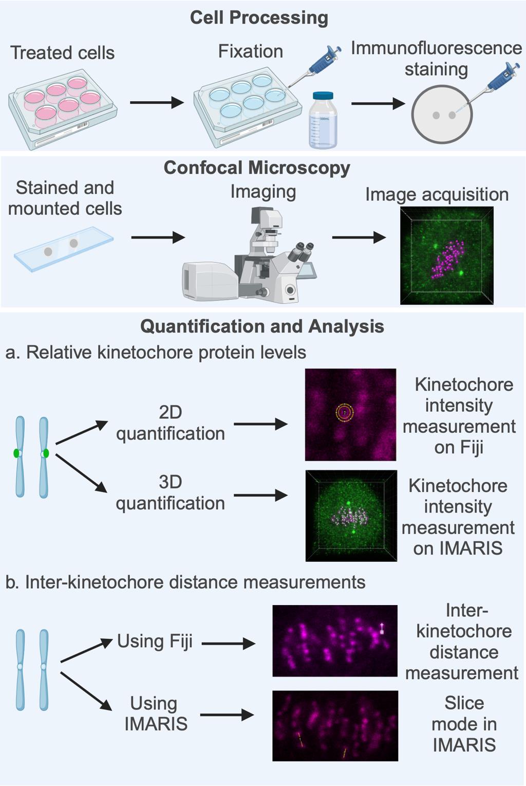
Key steps involved in fluorescence quantification of spindle assembly checkpoint (SAC) protein loading at the kinetochores and in the calculation of inter-sister kinetochore distances. High-resolution confocal image datasets of cells subjected to appropriate treatment as per the experimental need (drugs, inhibitors, gene-specific siRNA, etc.) are used for quantifying the levels of SAC proteins at the kinetochores, measuring inter-sister kinetochore distances, or both. Quantification and analysis of both parameters are performed using image analysis software such as Fiji (open source) or the IMARIS software suite. Figure created with BioRender.com.
Background
The spindle assembly checkpoint (SAC) is the primary mechanism that ensures equal sister chromatid segregation [1–3]. The SAC monitors two major parameters during mitosis. The first is the end-on attachment of centrosome-derived microtubule plus ends to the kinetochores (Kt-MT attachment). The establishment of bipolar (amphitelic) Kt-MT attachment of a sister chromatid pair to opposite centrosomes, followed by the depolymerization of these kinetochore microtubules (kMTs), leads to poleward pulling of the kinetochores and the generation of inter-kinetochore tension, the second parameter sensed by the SAC. All other stochastically occurring forms of Kt-MT mis-attachment (monotelic, merotelic, and syntelic) fail to elicit inter-kinetochore tension [1].
The SAC operates through SAC proteins resident on the fibrous corona, the outermost and most transient kinetochore layer. The SAC generates a diffusible “wait-anaphase” signal triggered by the lack of attachment or mis-attachment at even one kinetochore, stalling the entire cell in metaphase and providing time for the rectification of Kt-MT mis-attachments [3]. Inter-kinetochore tension stabilizes Kt-MT end-on attachments and also initiates a molecular signaling cascade instrumental for the separation of sister chromatids toward the opposite spindle poles (centrosomes) due to kMT depolymerization. Inactivation or silencing of the SAC, achieved primarily through dynein-based poleward “stripping” of SAC proteins from kinetochores along spindle microtubules upon Kt-MT attachment or tension, is essential for anaphase onset [1,3].
The level of enrichment of SAC proteins, their receptors, and other associated proteins at the kinetochores can serve as biochemical markers of the exact stage of mitosis or be used as indicators of specific defects in mitotic progression [4]. High-resolution confocal microscopy has been used to reliably quantify these levels and correlate them with the stage of mitosis, mainly because the size of human kinetochores is not optically diffraction-limited [5]. Kinetochore protein level quantification methods were initially developed on individual, two-dimensional confocal micrographs of single z-planes, taking into account local background fluorescence corrections around the kinetochores [5] and have been used extensively since. In recent years, this concept has been built upon to evolve widely used methods employing modern microscopy analysis software packages and three-dimensional image reconstructions [6–8]. Similar tools have been used to quantify inter-kinetochore distances at prometaphase and metaphase. These distance measurements have proven to be reliable correlates of inter-kinetochore tension, especially at late metaphase prior to segregation [1]. This article details state-of-the-art methodologies for the quantification of levels of kinetochore proteins and distance measurements between sister kinetochores. The methods described can be adapted to most cultured cells/cell lines that can be imaged using high-resolution confocal fluorescence microscopy.
Materials and reagents
Reagents
Immunofluorescence labeling
Primary antibodies against the protein(s) of interest (the Mad1 example is shown here):
Mad1 (Thermo Fisher Scientific, catalog number: PA5–28185). Other alternatives compatible with immunofluorescence staining may be used after empirical optimization.
CREST (to stain kinetochores) (Antibodies Incorporated, catalog number: 15–234). Other alternatives staining the kinetochore or the centromere that are compatible with immunofluorescence staining may be used after empirical optimization for specificity.
α-Tubulin, DM1 alpha (Sigma, catalog number: T9026)
Secondary antibodies tagged with fluorophore:
Alexa Fluor® 488 AffiniPure Donkey Anti-Rabbit IgG (Jackson ImmunoResearch Inc., catalog number: 711–545-152)
Alexa Fluor® 594 AffiniPure donkey Anti-Mouse IgG (Jackson ImmunoResearch Inc., catalog number: 715–585-150)
CyTM 5 AffiniPure Donkey Anti-Human IgG (Jackson ImmunoResearch Inc., catalog number: 709–175-149)
Note: Other alternative fluorophore-conjugated secondary antibodies compatible with immunofluorescence staining may be used after empirical optimization.
Sodium chloride (NaCl) (SRL, catalog number: 64072); may be procured commercially from other standard sources
Potassium chloride (KCl) (SRL, catalog number: 38630); may be procured commercially from other standard sources
Disodium hydrogen phosphate (Na2HPO4) (SRL, catalog number: 1949144); may be procured commercially from other standard sources
Potassium dihydrogen phosphate (KH2PO4) (SRL, catalog number: 1649201); may be procured commercially from other standard sources
Triton X-100 (Sigma, catalog number: T8787–100ML)
Bovine serum albumin (BSA) (pH 6–7) (SRL, catalog number 9048–46-8); may be procured commercially from other standard sources
4',6-diamidino-2-phenylindole (DAPI), 5 mg/mL stock solution made in dimethyl sulfoxide (DMSO) (Thermo Scientific, catalog number: 62247)
Note: Alternatively, chromatin dyes for immunofluorescence such as Hoechst 33342 may be used after empirical optimization.
ProLong DiamondTM mounting media (Thermo Scientific, catalog number: P36970). Alternative antifade mounting media with a refractive index compatible with the lens and the lens immersion medium may be used after empirical optimization
1× phosphate buffered saline (PBS) (see Recipes)
Blocking solution (see Recipes)
1× phosphate buffered saline (PBS)
Components Amount/volume added Working concentration NaCl 8 g 137 mM KCl 0.2 g 2.7 mM Na2HPO4 1.44 g 10 mM KH2PO4 0.24 g 2 mM Deionized water Make up the volume to 1 L Blocking solution for immunofluorescence staining
Components Amount/volume added Working concentration PBS 50 mL 1× Triton X-100 250 µL 0.5% BSA 0.5 g 1% Weigh 0.5 g of BSA and add to 45 mL of 1× PBS in a 50 mL tube.
Place the tube on a rocker and mix at slow speed until completely dissolved. Avoid frothing of the solution.
Caution: High-speed mixing can denature proteins including BSA, of which frothing is a sign.
Add 250 μL of Triton X-100 to the solution.
Slowly mix the solution on a rocker to dissolve all the components completely.
Add 1× PBS to make up the volume to 50 mL and gently mix to homogeneity.
Clean glass slides and coverslips
Critical: The coverslips should be properly cleaned and ideally be of category #1.5 (even thickness between 0.16 and 0.19 mm) to minimize chromatic aberration and refractive index mismatches between the lens, immersion medium, and sample mounting medium.
Equipment
Confocal image acquisition
Leica TCS SP8 laser scanning optical confocal microscope with HCX PL APO 63X-1.4 NA oil-immersion objective and a HyD (hybrid) or photomultiplier tube (PMT) detector.
Note: Equivalent confocal microscopes from standard commercial sources may be used, as long as they offer the following key features:
Plan apochromat (PL APO) confocal grade objectives with a high numerical aperture (1.2 or above).
Laser illumination in at least three distinct colors.
Emission pinhole(s) designed to block out-of-focus emission light from adjacent z-planes from being captured in the images.
In the case of raster laser scanning confocal scan-heads, high-sensitivity detectors such as PMTs, hybrid detectors, or avalanche photodiodes (APDs) with a quantum efficiency in the visible spectrum around 50 % may be used. Alternatively, for spinning disc confocal microscopes, high sensitivity cameras such as scientific complementary metal oxide semiconductor (sCMOS) cameras or electron multiplying charge-coupled device (EMCCD) cameras, with a quantum efficiency in the visible spectrum of around 80% or above, may be used.
Software and datasets
For image analysis
IMARIS software suite, version 8.3, Bitplane. Higher versions may be used.
Fiji (open-source image analysis software) (https://fiji.sc, Schindelin et al. [9])
For statistical analysis
GraphPad Prism (GraphPad Software, USA). Other standard software packages may be used.
Procedure
Cell fixation and immunofluorescence labeling
Note: Prior to fixation and immunofluorescence labeling, cells may be subjected to treatment as per experimental needs. For instance, siRNA-mediated protein depletion or using specific inhibitors against the protein of interest and subsequent scoring for mitotic phenotype(s) may suggest its role in cell division.
After treatment of the cells as per experimental requirements, remove the coverslips containing the cells and place them in a fresh 6-well plate with the surface containing the cells facing upward for further processing.
Wash the cells 2–3 times with 2 mL of 1× PBS each time.
Add 2–3 mL of pre-chilled (at -20 °C) absolute methanol (AR grade or HPLC grade) to the coverslips to fix the cells.
Immediately place the 6-well plate at -20 °C for a minimum of 30 min to complete the fixation process.
Note: The coverslips may be stored at -20 °C submerged in absolute methanol for an extended period of time without letting the methanol dry out.
Note: An alternate method of fixation has been described in the literature for mammalian cell kinetochores, using 4% formaldehyde and a buffer consisting of PIPES-HEPES-EDTA and magnesium chloride (PHEM) [10]. This method may be optimized and alternatively used. If this method of fixation is used, the following immunostaining steps must be immediately performed, since aldehyde fixation does not remain stable over long periods. Additionally, only 4% paraformaldehyde in 1× PBS may also be used for fixation prior to immunostaining [7, 8, 11].
Rehydrate the cells by adding adequate 1× PBS and wash 3–4 times (2 mL each time) to ensure complete rehydration.
Use a clean, fine-tipped pair of forceps to lift the coverslips and gently place them cell-side up on a fresh ParafilmTM sheet inside a humidified chamber prepared by lining a large cell culture dish with a damp paper towel and the lid closed.
Caution: All following steps are performed in the humidified chamber.
Add approximately 50–100 μL of blocking solution on each coverslip to cover the entire surface and leave at room temperature for 1 h. Only enough blocking solution should be added to form a large drop covering the entire coverslip.
Prepare the primary antibody solution by diluting all required primary antibodies (caution: raised in different animals) in blocking buffer in a fresh microcentrifuge tube (Mad1: 1:200, CREST: 1:100, α-tubulin: 1:800) at room temperature.
After 1 h of blocking, gently aspirate off the blocking solution from the edge of the coverslip to remove the blocking solution, add approximately 40–50 μL of diluted primary antibody to each coverslip, and incubate for 1 h at room temperature.
Note: 40 μL of the diluted antibody solution is sufficient to cover a 12 mm circle coverslip.
Remove the antibody solution and wash the cells thrice with blocking solution.
Dilute fluorophore-conjugated secondary antibodies (Alexa Fluor® 488 anti-rabbit IgG: 1:800, Alexa Fluor® 594 anti-mouse IgG: 1:800, and CyTM 5 anti-human IgG: 1:800) in a single microcentrifuge tube containing blocking solution and add 40–50 μL to each coverslip. Incubate at room temperature for 1 h.
Aspirate off the secondary antibody solution and wash the cells with 1× blocking solution thrice.
Wash cells with 1× PBS once to remove the blocking solution.
Add 50 μL of diluted DAPI (1:10,000 of a 5 mg/mL stock made in DMSO) and incubate for a maximum of 2 min at room temperature.
Aspirate off the DAPI solution and wash the cells thrice with 1× PBS.
Wash the cells once with de-ionized water to remove the PBS.
Note: The salts in the PBS can cause noise during fluorescence/confocal imaging and must therefore be removed.
Label a clean, frosted glass slide on the frosting using a lead pencil. Place 5 µL of ProLong DiamondTM mounting media on it. Gently lift the coverslips using forceps and drain any excess liquid by touching the bottom edge of the vertically held coverslip on a piece of lint-free tissue paper. Place the coverslip on the drop of mounting media (cell-side down) by laying it down gently from one edge and letting the weight of the coverslip spread the mounting media under it as it settles. Remove any trapped air bubbles between the coverslip and the slide by pushing them outward with gentle pressure on the coverslip using the tip of the forceps.
Allow the mounted coverslips to air-dry overnight at room temperature, protected from light on a flat, horizontal surface.
Caution: This step shouldnotbe performed in the humidified chamber.
The dried coverslips may be imaged immediately on a confocal microscope or stored at -20 °C in a slide box for later use.
Image acquisition
Acquire high resolution images of prometaphase and metaphase cells on a Leica TCS SP8 laser scanning optical confocal microscope (or equivalent) using an HC PL APO 63×-1.4 NA oil-immersion objective and a HyD (hybrid) or PMT detector.
Keep the imaging parameters constant for all experimental conditions using the Leica LASX software (or other acquisition software, as applicable).
Keep the zoom constant at 4.5× for imaging mitotic cells (both metaphase and prometaphase).
Use simultaneous scanning sequences for two different wavelength channels for image acquisition. Ensure that the emission wavelength of one fluorophore does not cross-excite any other fluorophore. For example, in scan sequence 1, use laser lines for 405 nm and 594 nm, and in scan sequence 2, use laser lines for 488 nm and 647 nm.
Note: Alternatively, image acquisition can be performed using sequential scanning to eliminate the possibility of inadvertent fluorophore cross-excitation. However, the scanning sequence should begin at the highest wavelength (647 nm) and end at the lowest wavelength (405 nm).
Critical: An important consideration during imaging for fluorescence quantification is to never expose the fluorophore tagged to the protein of interest while focusing or locating cells prior to image acquisition. This is important to prevent bleaching of the fluorophore when the laser hits the sample and may therefore impact accurate quantitative measurements.
Adjust the oversaturation and undersaturation of the emission signals using the Quick Look-up Table (QLUT) or an equivalent feature to stay within the dynamic range of the detectors (Table 1).
Table 1. Imaging parameters used during acquisition
Checklist of imaging parameter settings to be ensured before imaging S. no. Setting name Imaging parameters Remarks 1 Scan Mode xyz 2 Imaging resolution 1024 × 1024 The images should be acquired at high resolution for effective 2D and 3D quantification. 3 Scan Direction X Bidirectional For faster coverage of the imaged field. 4 Scan Speed 200 Hz Higher frequency (scan speed) enables faster coverage of the imaged field but can compromise image resolution. Caution: For kinetochore fluorescence quantification through fixed cell imaging, image resolution is more important than imaging speed. The software should clearly be able to tell the kinetochore apart from the background (this must be manually ascertained). 5 Magnification 63× Other companies use Plan Apochromat lenses of 60×/64× magnification, for which the parameters would remain similar. 6 Objective name and numerical aperture HC PL APO CS2 63×/1.40 NA (numerical aperture) oil immersion lens A higher NA lens provides better resolution. 7 Immersion Oil (Leica type F immersion liquid, catalog number: 11513859) An equivalent immersion oil/immersion liquid from other manufacturers may also be used. 8 Zoom [Region of Interest (ROI) imaging] 4.5 Keep the zoom factor such that only the dividing cell is imaged (zoom factor was kept at 4.5 in the Leica TCS SP8 microscope). In a laser scanning microscope, this reduces the area of the field that needs to be scanned, leading to faster imaging. 10 Pinhole diameter 0.5 Airy Units (AU) The pinhole diameter is usually set at 1 AU for most confocal microscopes. For kinetochore imaging, which usually shows bright fluorescence emission, a lower pinhole diameter (such as 0.5 AU) increases the x-y resolution. Caution: Lower pinhole diameters cannot be used for weak fluorescence intensity/signals. A good primary antibody that gives a strong and specific fluorescence signal must be used for immunostaining. 11 Scanning sequence 1 488 nm for antigen to be quantified and 647 nm for CREST The two fluorophores can be simultaneously excited, and the emission signals simultaneously captured on two separate detectors. 12 Scanning sequence 2 405 nm for DAPI and 594 nm for microtubules The two fluorophores can be simultaneously excited, and the emission signals simultaneously captured on two separate detectors. Use an imaging pixel format of 1024 × 1024 and a scan speed of 200 Hz for image acquisition. The higher pixel format enables higher image resolution and subsequent quantification of fluorescence intensities with greater accuracy.
If required, reduce the pinhole diameter to 0.5 Airy units (AU) for better structural definition of the kinetochores.
Note: Reducing the pinhole omits low emission intensities and can therefore be used only when the emission signal is strong.
Keep the z-step size at 0.3 μm.
Start image acquisition after ensuring all settings are accurate.
Acquire z-sections (optical depth section images) of each cell in steps of 0.3 μm each, starting from the first out-of-focus plane on one side of the cell, optically sectioning through the cell, and ending at the first out-of-focus z-plane on the other end of the cell.
Image analysis
Quantification of SAC proteins at the kinetochore can be achieved using 3D reconstruction of the z-slices in the IMARIS software suite. Alternatively, this can also be performed from 2D images as described in Hoffman et al. [5] using Fiji, Metamorph, or other software packages. Here, we describe the quantification of fluorescence intensities at the kinetochore both in 2D as well as in 3D. The schematics of the workflow are represented as flowcharts for fluorescence intensity measurements in 2D (Figure 1) and 3D (Figure 2).
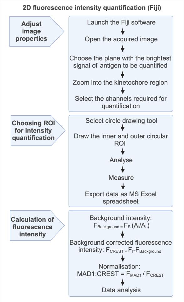
Figure 1. Schematic flowchart for fluorescence intensity measurement in 2D. Open the image in Fiji, select the z-plane with the brightest signal for SAC protein, zoom into the kinetochore area, draw a circular ROI (0.45 μm diameter) around the CREST signal, draw a circular ROI (0.63 µm diameter) around the CREST signal for background correction, measure fluorescence intensity (Analyze > Measure), and export all intensity values as an MS Excel spreadsheet for further analyses. Figure created with BioRender.com.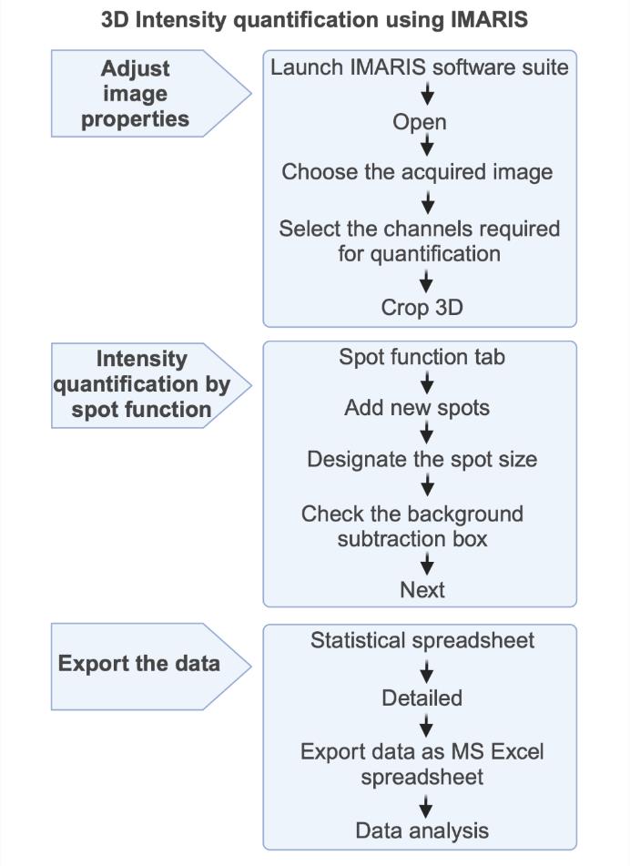
Figure 2. Schematic flowchart for fluorescence intensity measurement in 3D. Launch IMARIS software suite, open the image file, select the image to be analyzed, select the channel to be used for analysis, crop the cell in 3D, open the spot function, assign the spot size and add new spot, check the background subtraction box and click the next button, click the statistical spreadsheet followed by detailed button, and export all intensity values as an MS Excel spreadsheet for further analyses. Figure created with BioRender.com.The quantification of SAC protein levels at the kinetochore using 2D imaging (Fiji) is illustrated in Figure 3 with the following steps:
For quantification of SAC proteins at the kinetochore, consider cells that have clearly defined kinetochore immunofluorescence (as visualized using the CREST stain).
Open the selected cells in Fiji. Choose the z-plane(s) containing the visibly brightest signal for Mad1 (the SAC protein example illustrated here) by going through the entire z-stack and selecting the channels for CREST (resident kinetochore protein) and Mad1 for quantification.
Zoom into the kinetochore (chromosomal) region of the cell. It is important to maintain the same zoom for all channels to ensure the regions of interest (ROI) across channels have the same XY dimensions.
Draw a circular ROI of diameter 0.45 μm encompassing the CREST signal using the circular drawing tool from the Fiji menu bar and designate it as the inner circle.
Critical: The average size may be empirically determined for individual cell lines using several control kinetochores across multiple cells to capture the CREST (kinetochore) signal and the signal of the loaded kinetochore SAC protein. SAC proteins at kinetochores may not always be seen overlaid on the same exact pixels as the kinetochore antigen. The loading of these proteins can accumulate significantly on laterally adjacent pixels attached to the kinetochore, especially in prometaphase.
Draw a larger circle of 0.63 μm diameter (approximately double the area of the inner circle) around the inner circle and designate it as the outer circle. The fluorescence intensity from the outer circle will be used for calculating the local background during quantification.
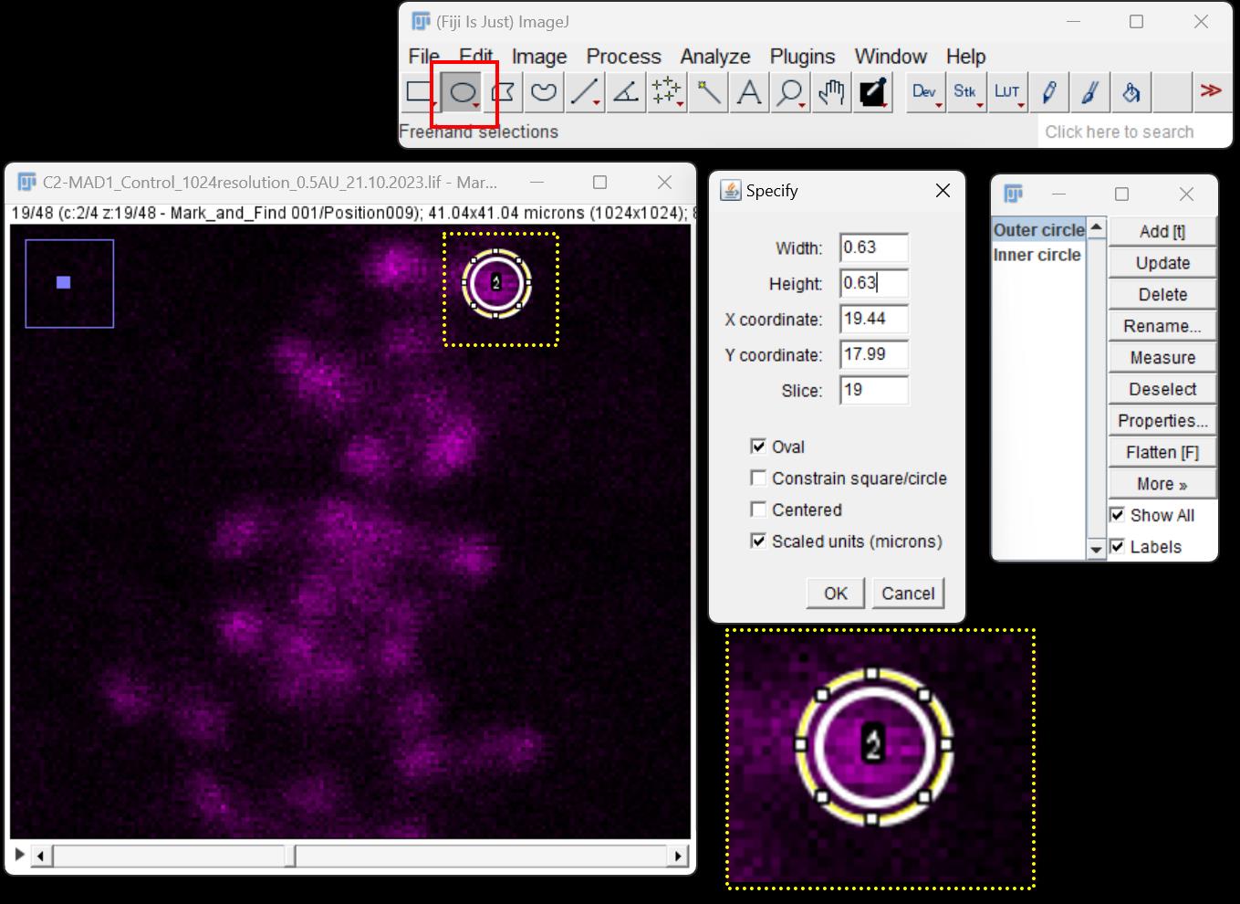
Figure 3. Fluorescence quantification of SAC protein loading at the kinetochore in 2D using Fiji image analysis software. The window on the far left is the confocal micrograph showing kinetochores (pseudo-colored in magenta). An ROI is drawn around the kinetochore using the tool shown in the red box. The diameter of each circular ROI is assigned in the window labeled Specify. The box labeled Scaled units (microns) is checked to convert the measurement of the circular ROI to micrometers. Each ROI is added to the ROI manager as shown in the window on the far right and designated as either outer circle or inner circle. The yellow dotted box represents ROIs drawn around each kinetochore to be quantified; the inset of the same represents the zoomed image.Once all ROIs are drawn, measure the fluorescence intensities using the Analyze > Measure tool on the Fiji menu bar. This generates a data sheet for all fluorescence intensities and can be exported as an MS Excel spreadsheet for further calculations.
Paste the ROIs from the CREST channel on the Mad1 channel and obtain fluorescence measurements for the Mad1 channel as described in step C6.
After exporting the fluorescence intensities from all channels to an MS Excel spreadsheet, perform the following calculations.
For calculating the fluorescence intensity of the region between the inner and the outer circles (FS), subtract the integrated fluorescence of the inner circle (FI) from the integrated fluorescence of the outer circle (FO).
Next, calculate the area of the region between the inner and outer circles (AS) by subtracting the area of the inner circle (AI) from the area of the outer circle (AO).
AS = AO - AI
Calculate the background intensity (FBackground) using the equation below:
FBackground = FS (AI/AS)
The background corrected fluorescence intensity of CREST is obtained by subtracting the background intensity (FBackground) from the intensity of the inner circle (FI).
FCREST = FI - FBackground
Calculate the final fluorescence intensity of Mad1 (FMad1) in the same manner by following steps C10–12 for the Mad1 channel.
Normalize the Mad1 intensity to the CREST intensity by dividing the background-corrected Mad1 intensity by the background-corrected CREST intensity for each kinetochore.
Mad1:CREST = FMad1/FCREST
The normalized ratio of Mad1:CREST is plotted as a scatter plot using GraphPad Prism.
Note: Other kinetochore resident proteins such as CENP-A and CENP-C (Cmentowski et al [12]) are also commonly used as kinetochore normalization markers. The underlying assumption is that the kinetochore structure and organization (inner and outer kinetochore layers) do not change upon SAC protein loading on the outermost fibrous corona in mitosis.
Quantification of inter-kinetochore distance (using Fiji)
Sequence of steps for fluorescence intensity measurement in 2D: Open image in Fiji > select z-plane with brightest signal for SAC protein > Analyze > line draw tool > draw line joining centroids of sister kinetochores > analyze > measure > export fluorescent intensities values as MS Excel spreadsheet for further analyses.
Inter-kinetochore distance is measured using Fiji in 2D.
Consider only those cells for quantification that have a tightly formed metaphase plate and in which most kinetochore pairs are aligned almost parallel to the spindle axis (the line connecting the two spindle poles). This is indicative of the late metaphase stage, where most kinetochores have captured microtubules and sufficient inter-kinetochore tension has been generated.
Select a single z-plane containing the highest number of visibly brightest CREST signals by moving across the z-stack.
Select the line draw tool from the Analyse tab on the Fiji menu bar and draw a straight line joining the centroids of a pair of kinetochores on the sister chromatids. This is illustrated in Figure 4.
The morphological features that characterize mammalian kinetochores are a faint, comet-like tail of CREST intensity connecting the two kinetochores. A pair of sister kinetochores (located on sister chromatids) is determined by moving through the z-stack. Adjacent CREST signals that come into and go out of focus in the same frame while moving through the z-stack are presumed to be a pair and therefore may be considered for distance measurements.
The distance between the pair of kinetochores is measured by selecting the Analyze > Measure tool on the Fiji menu bar. This generates a data sheet for inter-kinetochore distance in micrometers and can be exported as an MS Excel spreadsheet.
Twenty pairs of kinetochores per cell over a total of 20 cells per replicate are analyzed in this manner to obtain statistically significant data.
The distance measurements between kinetochore pairs from a set of experiments are plotted as a scatter plot using the GraphPad Prism software.
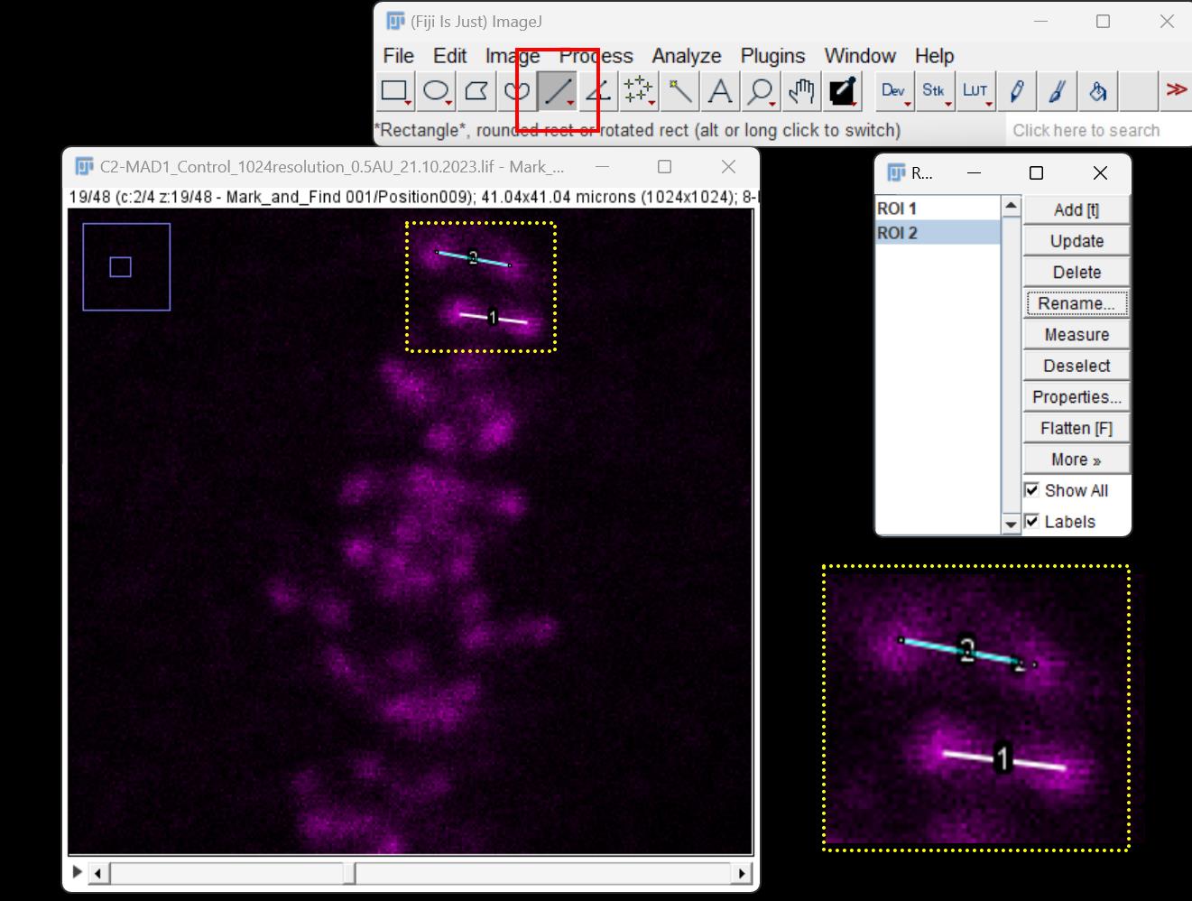
Figure 4. Quantification of inter-kinetochore distance in 2D using Fiji image analysis software. The window on the far left is the confocal micrograph showing kinetochores (pseudo-colored in magenta). A line connecting the centers of each pair of kinetochores (ROI) is drawn using the line tool (red box). The yellow dotted box highlights the representative lines drawn to connect the centers of two kinetochores, whose inset represents the zoomed form. Each ROI is added to the ROI manager (window on the far right) for calculating the inter-kinetochore distance.
Quantification of SAC protein(s) at the kinetochore in 3D
A flowchart depicting fluorescence intensity measurement steps in 3D is shown in Figure 2.
The IMARIS software suite is used for fluorescence quantification of SAC proteins at the kinetochore.
Launch the IMARIS software suite and open the acquired images using the Open tab on the menu bar as indicated in Figure 5 (yellow box).
A window containing all the acquired images appears. Open the image file from the list in the dialogue box as shown in figure 6.
Upon opening the selected image file, a 3D rendered image containing the xyz coordinates and all channels for that image (405 nm, 488 nm, 594 nm, and 647 nm) is displayed as below (Figure 7). Since channels for DAPI (405 nm) and microtubules (594 nm) are not considered for quantification of SAC proteins at the kinetochore, turn off these channels. Now, only signals for CREST in magenta (594 nm) and Mad1 (SAC protein) in green (488 nm) are displayed (Figure 8).
Select the Crop 3D option from the menu bar for cropping a cell in 3D. Carefully select the cell of interest using the selection tool, ensuring the exclusion of unwanted neighboring or background cells. Apply the cropping function by clicking OK to display only the 3D-cropped image (Figure 9).
Select the Spot function tab and press add new spot button as indicated in Figure 10 (yellow box). Once the Spot function is activated, a new window appears, as indicated in Figure 10 (yellow box).
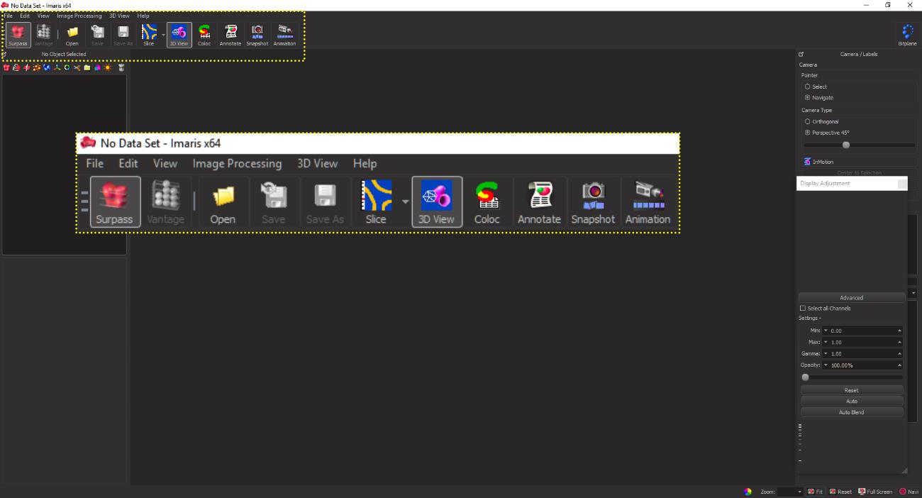
Figure 5. The graphical user interface (GUI) of the IMARIS software suite. The yellow dotted box and inset show the menu bar functions for opening the confocal image files for initiating the analysis.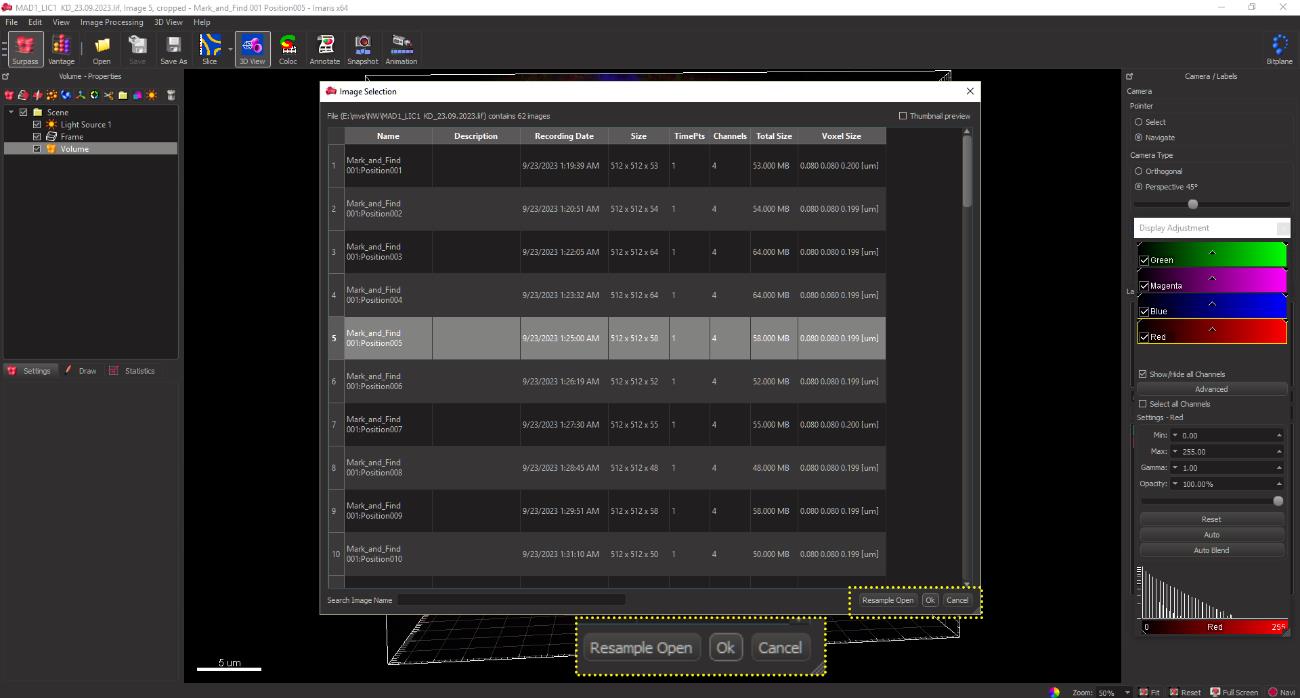
Figure 6. GUI of the IMARIS software suite showing the acquired confocal image files, enabling the user to select an image for analysis and open the selected file from the displayed dialogue box (yellow dotted box).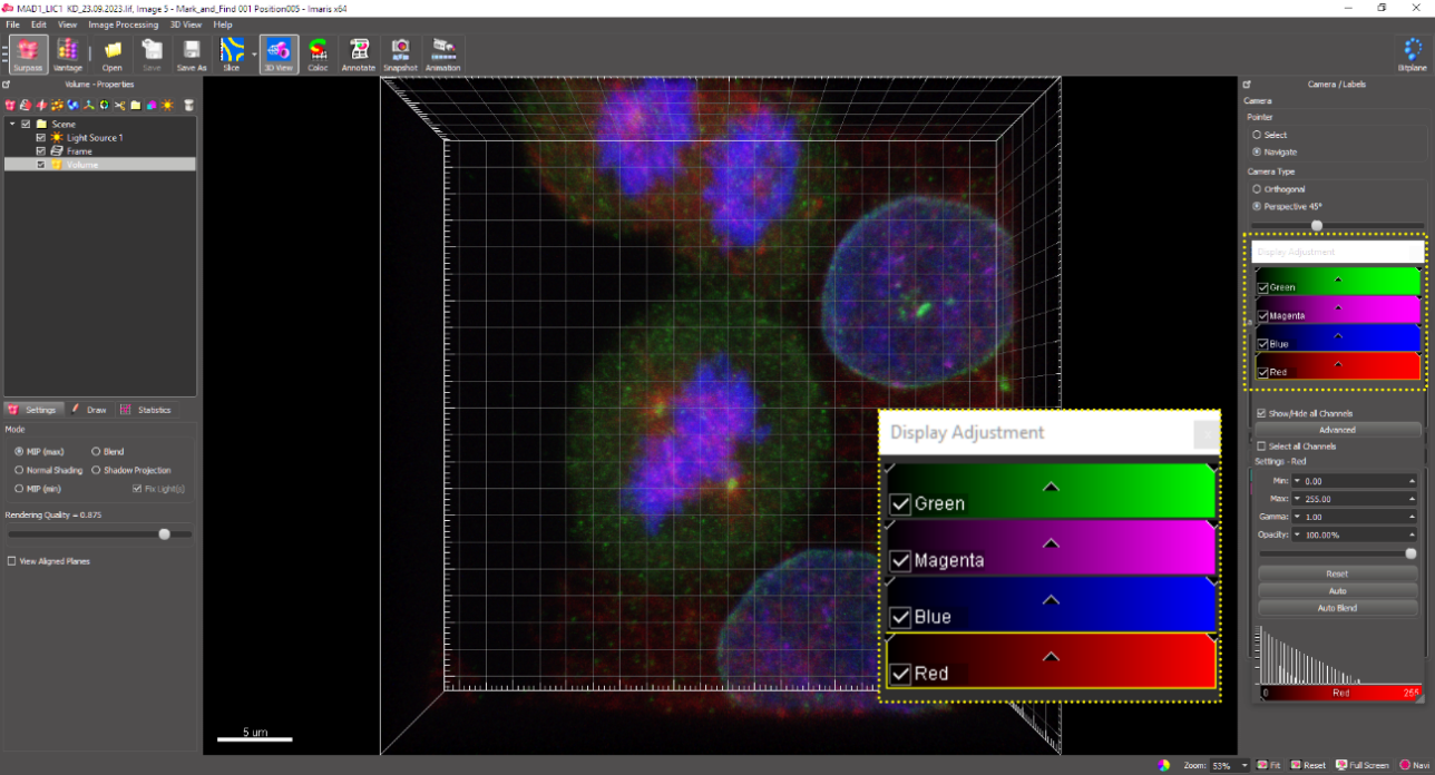
Figure 7. 3D reconstruction of the acquired confocal image displaying the xyz spatial coordinates and fluorescence channel information: Mad1 (green), CREST (magenta), DAPI (blue), and microtubules (red).
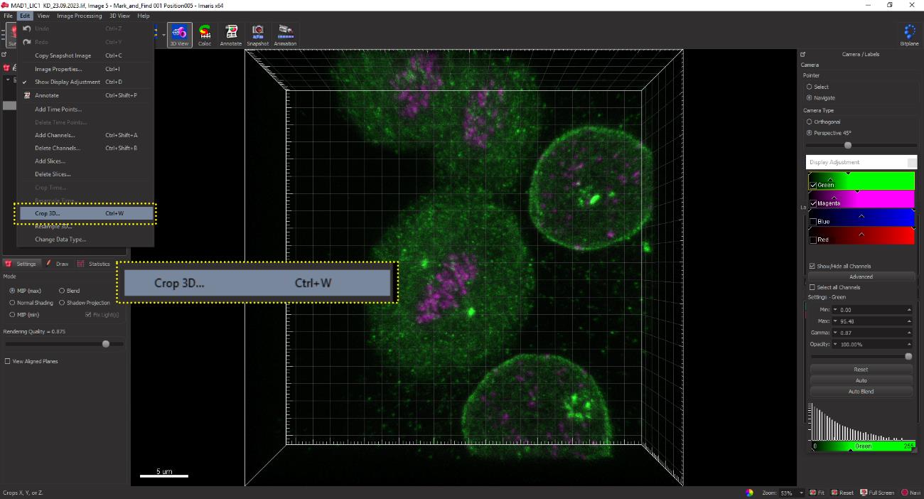
Figure 8. 3D cropping of the selected image. Click the edit button on the menu bar and click on the Crop 3D button from the dropdown menu for cropping the cell of interest in 3D. This function retains the x, y, z information of the selected image upon cropping.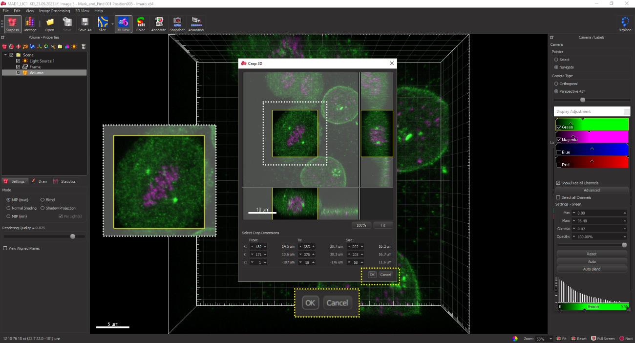
Figure 9. 3D cropping of the selected image. The white dotted box represents the region containing the cell of interest to be cropped in 3D. The OK button at the bottom right (yellow dotted box) enables the cropping of the cell of interest.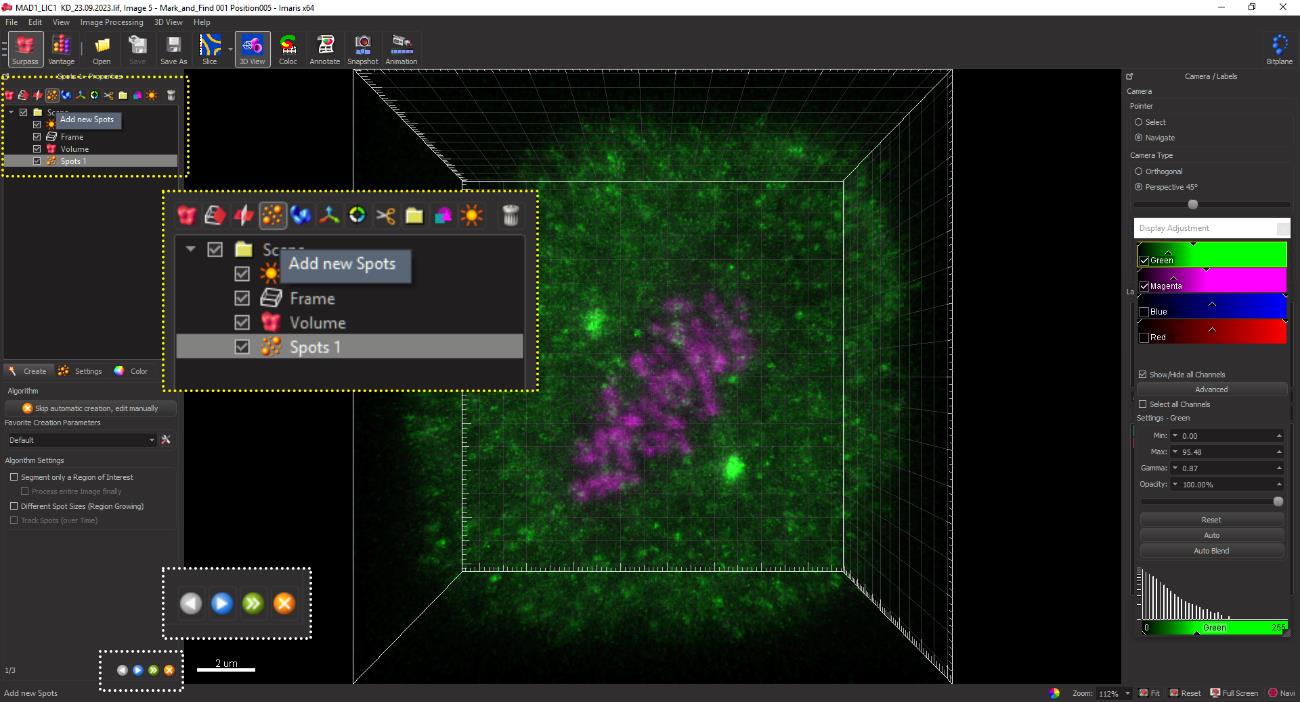
Figure 10. Activating the spot function on the IMARIS GUIThe channel for CREST (magenta) is selected, and the spot size of 0.45 μm is designated for kinetochores of HeLa cells. Also, the background subtraction box is checked to ensure that the software automatically subtracts the background fluorescence in the processed image (figure 11).
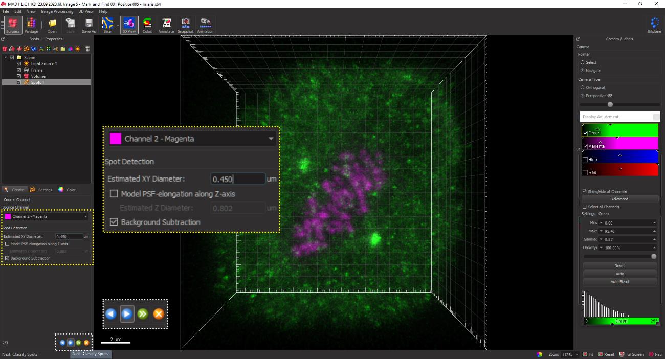
Figure 11. Assigning the spot size for kinetochores. Kinetochores are assigned a spot size of 0.45 μm in the selected channel for CREST (magenta) in HeLa cells. The average size may be empirically determined for individual cell lines using several control kinetochores across multiple cells to capture the CREST (kinetochore) signal and the signal of the loaded kinetochore SAC protein.The software automatically picks CREST-positive spots and displays them as grey balls. Spurious spots may also be occasionally picked by the software but can be manually deleted by adjusting the slider for the intensity (Figure 12, yellow inset box at the bottom). Conversely, spots that are clearly identified as kinetochores but may have been missed by the software can be added manually using the slider shown in the yellow dotted box in Figure 12.
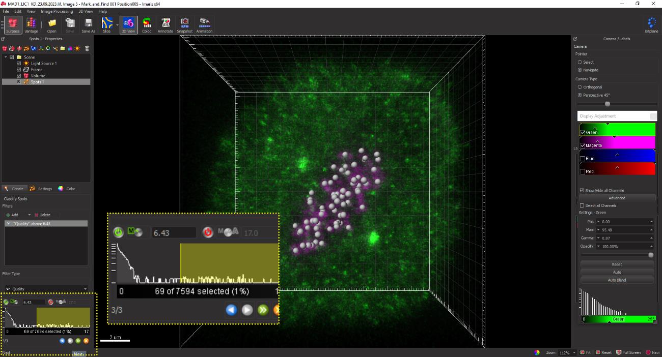
Figure 12. Kinetochore spots of 0.45 μm diameter as rendered in grey by the spot function on IMARIS. The yellow dotted box displays the interactive slider for selectively removing non-specific spots.Once all kinetochores have been selected, click the Next button to convert the grey spots to magenta as indicated in Figure 13.
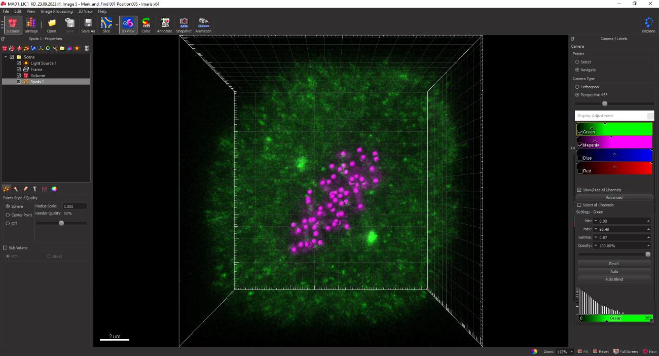
Figure 13. Finalizing the selected kinetochore spotsClick the statistical spreadsheet button followed by the detailed option button to simultaneously obtain the intensity sum values for the selected kinetochores (CREST) as well as the SAC protein loaded on the kinetochores (Mad1) (Figure 14, yellow dotted box).
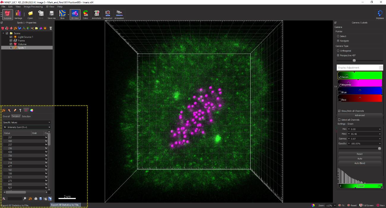
Figure 14. Fluorescence intensity sum values of the CREST and Mad1 channels are displayed in the yellow dotted box.Integrated intensity sum values for each spot for CREST and Mad1 are exported as an MS Excel spreadsheet for further calculations, as indicated in Figure 15.
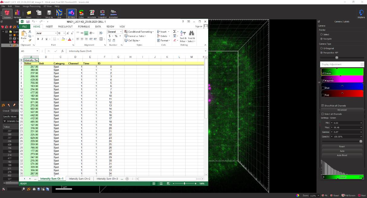
Figure 15. Screenshot of MS Excel spreadsheet displaying the quantified integrated fluorescence intensity measurements extracted for CREST and Mad1 as measured by IMARIS.For quantifying the level of Mad1 at the kinetochore, the ratio of the fluorescence intensities of Mad1:CREST is calculated for each spot by dividing the fluorescence intensity of Mad1 by that of CREST. These values are then sorted from high to low and the top 20 kinetochore intensity values are considered for each cell. These calculations are performed for at least 20 cells per replicate to obtain robust, statistically significant data.
Quantification of inter-kinetochore distance in 3D
Import the acquired raw image file into the IMARIS software suite. Access the file menu located in the upper left corner. Click on Open file to open the confocal image files containing all the acquired images and select and open the individual z-image to be quantified (single confocal plane). Click the OK button to open the selected image (yellow box, Figure 16).
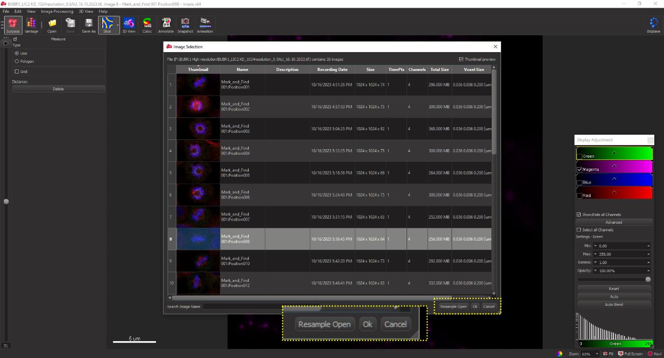
Figure 16. IMARIS GUI displaying the confocal image file containing all acquired images. An individual image can be selected and opened by clicking on the image followed by clicking OK.Select the Slice mode from the software menu bar. Since only the kinetochore channel (CREST, 647 nm) is required for quantification of inter-kinetochore distances, turn off all the other channels by un-checking the individual boxes as shown in Figure 17 (yellow dotted box).
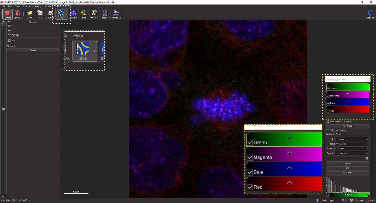
Figure 17. The presented image depicts a 2D confocal microscopy reconstruction, visualized using x, y, and z spatial coordinates. The image displays various fluorophore markers: Mad1 (green), CREST (magenta), DAPI (blue), and microtubules (red).Crop the cell of interest by selecting Crop 3D from the Edit button on the menu bar as described in step E5.
Zoom into the chosen metaphase cell such that the individual kinetochores are clearly visible. The morphological features that characterize mammalian kinetochores are a faint, comet-like tail of CREST intensity connecting the two kinetochores. A pair of kinetochores of sister chromatids is determined by moving through the z-stack. Adjacent CREST signals that come into and go out of focus at the same time while moving through the z-stack are presumed to be a pair and therefore may be considered for distance measurement (Figure 18).
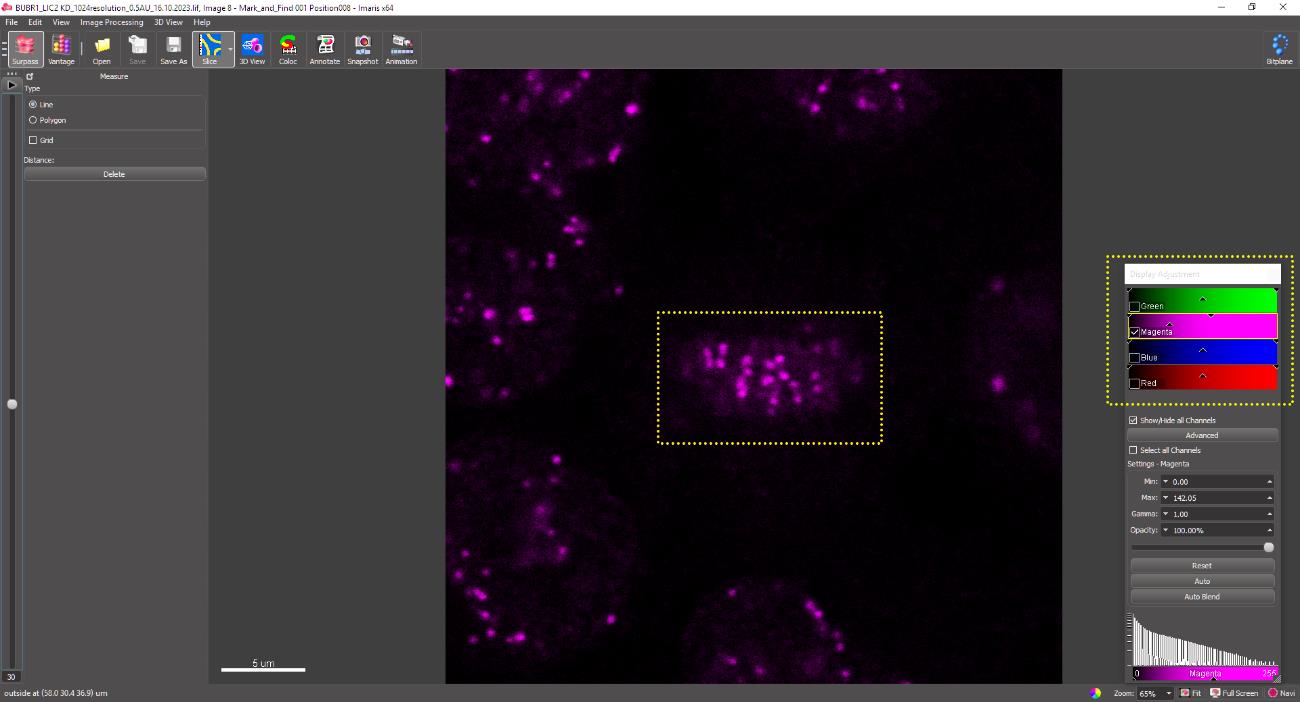
Figure 18. The yellow box depicts a metaphase cell containing pairs of sister kinetochores aligned at the metaphase plateClick on the center of each kinetochore pair. A line joining the two sister kinetochores appears as shown in Figure 19. The inter-kinetochore distance (here, 0.922 μm) appears in the dialogue bar in the upper-left corner (yellow box). Repeat for each kinetochore pair for all experimental conditions and record the values in an MS Excel spreadsheet. A minimum of 20 kinetochore pairs from each cell and 20 cells from each replicate are measured to obtain statistically significant data.
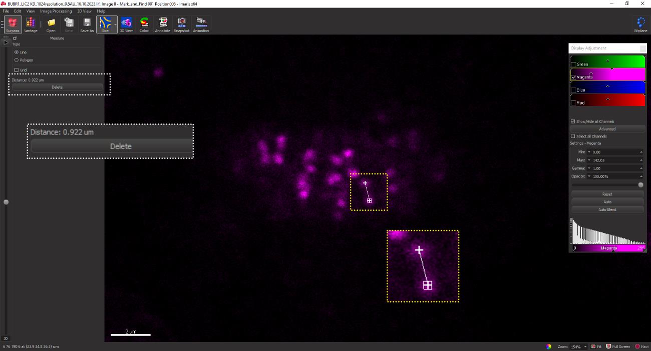
Figure 19. A specific z-plane is identified where two CREST spots from a pair of kinetochores are clearly discernible within the yellow dotted box. This z-plane is selected for the quantification of interkinetochore distance. The measured distance between the kinetochores of a pair is displayed in the box demarcated by the white dotted line (top left).The measurements obtained following the described method are represented as a scatter plot using the GraphPad Prism software.
Data analysis
Statistical analysis
A minimum of 20 kinetochore pairs from each cell and 20 cells from each replicate are analyzed for robust statistics as indicated in steps D7, E12, and F5. The distribution of the data is tested for normality using tests such as the D’Agostino–Pearson through the GraphPad Prism software. Parametric tests are used for normal data distribution (Student’s t-test/one-way ANOVA), while non-parametric tests are used for non-normal data distribution (Mann-Whitney U/Kruskal–Wallis) to statistically analyze the data and calculate statistical significance using the Prism software. Graphs are generated using the GraphPad Prism software. Error bars can be represented as standard deviation (SD) or standard error of mean (SEM) from at least three independent experiments (biological replicates)
Validation of protocol
Validation of quantitative analyses of fluorescence intensity
The methods described in this paper are widely accepted and have been used in the fields of kinetochore and mitosis biology for over twenty years [2, 5–8, 12–15]. However, users of either method may choose to cross-validate them. For instance, data using 2D quantification [13] and 3D quantification [6,7] of SAC proteins (Zw10, Mad1) upon depletion of the same gene (hLIC1) in the same cell type (HeLa) show reproducible phenotypes across the two methods.
General notes and troubleshooting
General notes
Cell fixation and immunofluorescence labeling
Mitotic cells are very loosely adherent to the substratum (coverslips). Therefore, very gentle washing using 1× PBS is recommended to avoid detachment of the mitotic cells.
Chilled methanol-fixed coverslips can be stored at -20 °C for an extended time as long as they stay immersed in chilled methanol throughout. However, if cells are fixed using aldehydes (4% formaldehyde or PHEM buffer), it is recommended that immunofluorescence staining be performed immediately.
After fixation using chilled methanol, rehydrate the cells adequately using 1× PBS for optimal immunostaining.
Prior to mounting the stained coverslips in mounting medium, it is crucial to remove all traces of PBS, as the salt crystals formed on the coverslips during the drying process may auto-fluoresce upon exposure to laser light and interfere during image acquisition.
Analysis from unevenly stained samples should be avoided. It is advisable to repeat the experiment and stain again to obtain even staining.
Image acquisition
If high background fluorescence is observed, a new experiment with a reduced concentration of the primary antibody is recommended for staining (needs to be empirically optimized). This is likely to reduce the non-specific signal.
If antibody signals remain non-specific, the use of fluorescently tagged constructs can be explored, with appropriate negative controls to rule out tag-induced artifacts.
Imaging parameters should be kept constant for all experimental conditions to ensure unbiased fluorescence quantification and data interpretation.
A zoom factor of 4.5 is optimal for imaging mitotic cells at sub-cellular resolution when using a 63× magnification plan apochromat lens.
While setting up simultaneous scanning sequences for multiple fluorophores, it is critical to ensure that the excitation and emission wavelengths of the two fluorophores are sufficiently far apart. This will minimize the chances of inadvertent cross-excitation of the lower energy fluorophore by the fluorescence emission of the higher energy fluorophore.
It is important to never expose the fluorophore channel of interest (which is to be quantified) to the laser while locating or focusing the field of cells to prevent any photo-bleaching of the fluorophore. This may significantly impact fluorescence quantification and data interpretation.
Oversaturation as well as undersaturation of fluorescence signals should be avoided during image acquisition. The Quick Look Up Table (QLUT, for Leica confocal microscopes) or an equivalent feature in other machines should be used to optimize the excitation light intensity and the detector gain voltage, in order to stay within the dynamic range of the detector.
The confocal pinhole aperture is normally set at 1 Airy unit. However, for strong emission signals, it may be adjusted to a lower value (such as 0.5 Airy units) to increase the lateral (x-y) resolution of the kinetochores being imaged.
In case a low emission signal-to-noise ratio (SNR) is observed, the following steps can be taken to improve the SNR: i) Increase detector gain voltage (detector sensitivity), not exceeding 700–800 V. Try not to increase the laser illumination intensity to avoid bleaching. ii) If required, increase the laser illumination intensity through the acoustic-optical tunable filter (AOTF) to a level where the SNR improves but bleaching does not happen.
Acknowledgments
The authors express gratitude to the Regional Centre for Biotechnology, India, for infrastructure, cell culture, and imaging facilities. N.W., M.S., and S.K. are supported by doctoral research fellowships from the Indian Council of Medical Research (ICMR) India, the Council for Scientific and Industrial Research (CSIR) India and the Department of Biotechnology (DBT) India, respectively, while S.M. is supported by a Women-in-Science (WOS-A) grant from the Department of Science and Technology (DST) India. This work was supported by funding to SVSM from the Department of Biotechnology (DBT; grant BT/PR6420/GBD/27/435/2012), the Science and Engineering Research Board (grants EMR/2016/007842 and CRG/2021/006858) and the Regional Centre for Biotechnology.
Author contributions: N.W., M.S., S.K., and S.M. conducted the experiments and analyzed data. N.W., M.S., and S.K. prepared figures. S.M. wrote and edited the manuscript. SVSM conceived, designed, supervised the study and edited the manuscript.
Competing interests
Authors declare no conflicts of interest or competing interests.
Ethical considerations
This study did not require any animal or human ethics clearances. The study was performed with due approval from the institutional biosafety committee of the Regional Centre for Biotechnology.
References
- McAinsh, A. D. and Kops, G. J. P. L. (2023). Principles and dynamics of spindle assembly checkpoint signalling. Nat Rev Mol Cell Biol. 24(8): 543–559. https://doi.org/10.1038/s41580–023-00593-z
- Cheeseman, I. M. and Desai, A. (2008). Molecular architecture of the kinetochore–microtubule interface. Nat Rev Mol Cell Biol. 9(1): 33–46. https://doi.org/10.1038/nrm2310
- Musacchio, A. and Salmon, E. D. (2007). The spindle-assembly checkpoint in space and time. Nat Rev Mol Cell Biol. 8(5): 379–393. https://doi.org/10.1038/nrm2163
- Howell, B., Hoffman, D., Fang, G., Murray, A. and Salmon, E. (2000). Visualization of Mad2 Dynamics at Kinetochores, along Spindle Fibers, and at Spindle Poles in Living Cells. J Cell Biol. 150(6): 1233–1250. https://doi.org/10.1083/jcb.150.6.1233
- Hoffman, D. B., Pearson, C. G., Yen, T. J., Howell, B. J. and Salmon, E. (2001). Microtubule-dependent Changes in Assembly of Microtubule Motor Proteins and Mitotic Spindle Checkpoint Proteins at PtK1 Kinetochores. Mol Biol Cell. 12(7): 1995–2009. https://doi.org/10.1091/mbc.12.7.1995
- Kumari, A., Kumar, C., Pergu, R., Kumar, M., Mahale, S. P., Wasnik, N. and Mylavarapu, S. V. (2021). Phosphorylation and Pin1 binding to the LIC1 subunit selectively regulate mitotic dynein functions. J Cell Biol. 220(12): e202005184. https://doi.org/10.1083/jcb.202005184
- Mahale, S. P., Sharma, A. And Mylavarapu, S. V. (2016), Dynein Light Intermediate Chain 2 Facilitates the Metaphase to Anaphase Transition by Inactivating the Spindle Assembly Checkpoint. PLoS One. 11(7):e0159646. https://doi.org/10.1371/journal.pone.0159646
- Bomont, P., Maddox, P., Shah, J. V., Desai, A. B. and Cleveland, D. W. (2005). Unstable microtubule capture at kinetochores depleted of the centromere-associated protein CENP-F. EMBO J. 24(22): 3927–3939. https://doi.org/10.1038/sj.emboj.7600848
- Schindelin, J., Arganda-Carreras, I., Frise, E., Kaynig, V., Longair, M., Pietzsch, T., Preibisch, S., Rueden, C., Saalfeld, S., Schmid, B., et al. (2012). Fiji: an open-source platform for biological-image analysis. Nat Methods. 9(7): 676–682. https://doi.org/10.1038/nmeth.2019
- DeLuca, K. F., Herman, J. A. and DeLuca, J. G. (2016). Measuring Kinetochore–Microtubule Attachment Stability in Cultured Cells. Methods Mol Biol. 1413: 147–168. https://doi.org/10.1007/978–1-4939–3542-0_10
- Martinez-Exposito, M. J., Kaplan, K. B., Copeland, J. and Sorger, P. K. (1999). Retention of the Bub3 checkpoint protein on lagging chromosomes. Proc Natl Acad Sci USA. 96(15): 8493–8498. https://doi.org/10.1073/pnas.96.15.8493
- Cmentowski, V., Ciossani, G., d'Amico, E., Wohlgemuth, S., Owa, M., Dynlacht, B. and Musacchio, A. (2023). RZZ‐Spindly and CENP‐E form an integrated platform to recruit dynein to the kinetochore corona. EMBO J. 42(24): e2023114838. https://doi.org/10.15252/embj.2023114838
- Sivaram, M. V. S., Wadzinski, T. L., Redick, S. D., Manna, T. and Doxsey, S. J. (2009). Dynein light intermediate chain 1 is required for progress through the spindle assembly checkpoint. EMBO J. 28(7): 902–914. https://doi.org/10.1038/emboj.2009.38
- Trivedi, P., Palomba, F., Niedzialkowska, E., Digman, M. A., Gratton, E. and Stukenberg, P. T. (2019). The inner centromere is a biomolecular condensate scaffolded by the chromosomal passenger complex. Nat Cell Biol. 21(9): 1127–1137. https://doi.org/10.1038/s41556–019-0376–4
- Weber, J., Legal, T., Lezcano, A. P., Gluszek-Kustusz, A., Paterson, C., Eibes, S., Barisic, M., Davies, O. R. and Welburn, J. P. (2024). A conserved CENP-E region mediates BubR1-independent recruitment to the outer corona at mitotic onset. Curr Biol. 34(5): 1133–1141.e4. https://doi.org/10.1016/j.cub.2024.01.042
Article Information
Publication history
Received: Apr 8, 2024
Accepted: Sep 30, 2024
Available online: Nov 4, 2024
Published: Dec 5, 2024
Copyright
© 2024 The Author(s); This is an open access article under the CC BY-NC license (https://creativecommons.org/licenses/by-nc/4.0/).
How to cite
Readers should cite both the Bio-protocol article and the original research article where this protocol was used:
- Wasnik, N., Singhal, M., Khantwal, S., Mylavarapu, S. and Mylavarapu, S. V. S. (2024). Quantitative Analysis of Kinetochore Protein Levels and Inter-Kinetochore Distances in Mammalian Cells During Mitosis. Bio-protocol 14(23): e5132. DOI: 10.21769/BioProtoc.5132.
- Kumari, A., Kumar, C., Pergu, R., Kumar, M., Mahale, S. P., Wasnik, N. and Mylavarapu, S. V. (2021). Phosphorylation and Pin1 binding to the LIC1 subunit selectively regulate mitotic dynein functions. J Cell Biol. 220(12): e202005184. https://doi.org/10.1083/jcb.202005184
Category
Cell Biology > Cell imaging > Confocal microscopy
Cell Biology > Cell-based analysis
Do you have any questions about this protocol?
Post your question to gather feedback from the community. We will also invite the authors of this article to respond.