- Protocols

- Articles and Issues
- For Authors
- About
- Become a Reviewer

Quantitative Analysis of Fish Morphology Through Landmark and Outline-based Geometric Morphometrics with Free Software
Published: Vol 14, Iss 20, Oct 20, 2024 DOI: 10.21769/BioProtoc.5087 Views: 2434
Reviewed by: Olga KopachSergii RomanenkoAnonymous reviewer(s)
Advertisement


Protocol Collections
Comprehensive collections of detailed, peer-reviewed protocols focusing on specific topics


Abstract
Morphology underpins key biological and evolutionary processes that remain elusive. This is in part due to the limitations in robustly and quantitatively analyzing shapes within and between groups in an unbiased and high-throughput manner. Geometric morphometrics (GM) has emerged as a widely employed technique for studying shape variation in biology and evolution. This study presents a comprehensive workflow for conducting geometric morphometric analysis of fish morphology. The step-by-step manual provides detailed instructions for using popular free software, such as the TPS series, MorphoJ, ImageJ, and R, to carry out generalized Procrustes analysis (GPA), principal component analysis (PCA), discriminant function analysis (DFA), canonical variate analysis (CVA), mean shape analysis, and thin plate spline analysis (TPS). The Momocs package in R is specifically utilized for in-depth analysis of fish outlines. In addition, selected functions from the dplyr package are used to assist in the analysis. The full process of fish outline analysis is covered, including extracting outline coordinates, converting and scaling data, defining landmarks, creating data objects, analyzing outline differences, and visualizing results. In conclusion, the current protocol compiles a detailed method for evaluating fish shape variation based on landmarks and outlines. As the field of GM continues to evolve and related software develops rapidly, the limitations associated with morphological analysis of fish are expected to decrease. Interoperable data formats and analytical methods may facilitate the sharing of morphological data and help resolve related scientific problems. The convenience of this protocol allows for fast and effective morphological analysis. Furthermore, this detailed protocol could be adapted to assess image-based differences across a broader range of species or to analyze morphological data of the same species from different origins.
Key features
• This protocol provides a comprehensive set of commonly used GM-analyzing methods and visualizing skills plus supporting information to help assess the appropriate analysis method
• By incorporating both landmarks and outlines, this protocol facilitates a thorough analysis of two-dimensional shape variation in fish, covering a wide range of morphological features
• The simplified workflow and detailed procedures make it accessible for non-experienced users to successfully complete the analysis while also providing valuable insights for experienced users
Keywords: Morphological variationGraphical overview
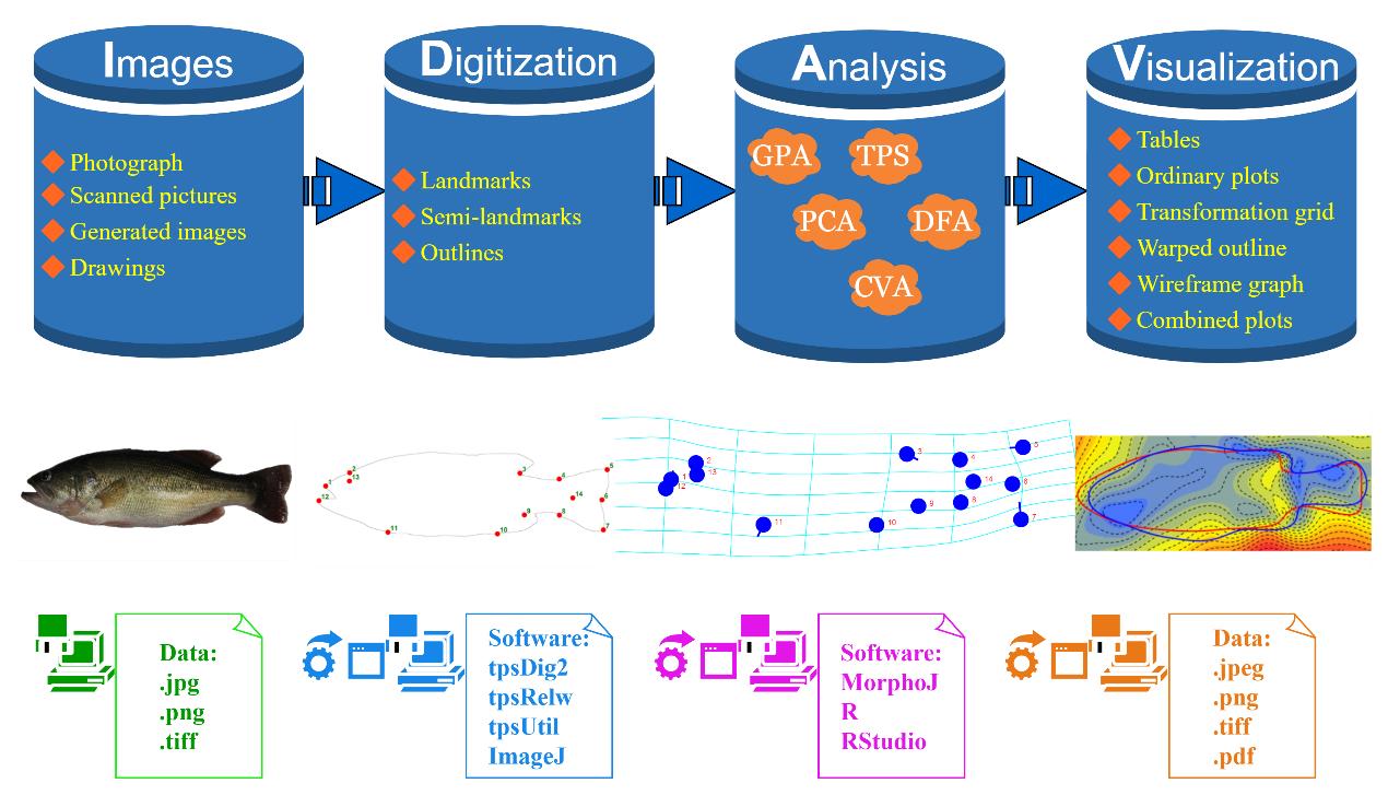
Workflow for conducting geometric morphometrics analysis on fish. The steps include image acquisition as data sources, digitization of fish morphology using landmark-based methods, analysis of shape variation characteristics, and visualization of the results in relation to biological interpretation. Largemouth bass (Micropterus salmoides) is used as an example in the schematic representation.
Background
Morphology has long been recognized as a fundamental trait in the field of biology. The intricate relationship between morphogenetic and evolutionary factors, as well as morphospaces, underscores the need for multivariate methods in biological and ecological research [1]. Geometric morphometrics (GM) has emerged as a widely utilized approach for the quantitative analysis of shape variation, particularly in the domains of biology and anthropology. It has become one of the primary methods for assessing essential morphological variables because it provides a quantitative/unbiased approach and morphological comparison [2]. GM has been instrumental in addressing a diverse array of questions related to morphological variation, including population differences, developmental patterns, responses to environmental factors, evolutionary trends, and functional morphology. Within the realm of morphology, three styles of morphometrics are commonly employed: traditional morphometrics, landmark-based GM, and outline-based GM [3]. In general, GM encompasses the following analytical steps: data acquisition, morphological variation analysis, results visualization, and interpretation.
For novice practitioners, the intricacy of GM often arises from the complexities associated with data construction and transformation, as well as the diverse array of analyzing methods available. Throughout the process, landmarks serve as the foundation for quantifying shape. GM analysis can be conducted using distinct landmark configurations for landmarks and semi-landmarks [4]. Traditionally, there are three types of landmarks [5]. However, as GM has advanced, the classification system for landmarks has evolved, with a more convenient typology being utilized in applied studies [6,7]. In the updated typology, the conventional roster of landmark points can be categorized into six types, intended to supersede the three types outlined in Bookstein [5]. This new classification corresponds to the different operational origins of the points along the curve or curves on which they are situated [6]. The process of landmarking and classifying landmarks may heavily rely on biological interpretation, and the major limitation of these types of techniques is that the labeling-analysis processes are all semi-manual or manual. Nevertheless, landmarking analysis remains the primary technique used in GM to this day. The characteristics of landmarks are described below.
Type I landmarks (anatomical landmarks)
Definition:
Points of clear biological or anatomical significance that can be precisely and consistently identified across all specimens.
These landmarks correspond to specific, discrete, and easily recognizable anatomical features.
Examples:
The tip of the nose.
The corner of the eye.
The junction between bones.
Advantages:
High reliability and repeatability.
Easily comparable across specimens due to clear homology.
Applications:
Frequently used in studies of skeletal morphology and other well-defined anatomical structures.
Type II landmarks (mathematical landmarks)
Definition:
Points defined by geometric properties such as maxima or minima of curvature, or points where certain geometric properties change.
These landmarks may not correspond to specific anatomical features but are identified based on their geometric properties.
Examples:
The point of maximum curvature along a bone.
The deepest point in a notch.
Advantages:
Useful for capturing shape information where anatomical landmarks are not clearly defined.
Can provide additional geometric context to the shape.
Applications:
Often used in conjunction with Type I landmarks to provide a more comprehensive shape analysis.
Type III landmarks (constructed landmarks)
Definition:
Points defined by their relative position or constructed based on other landmarks.
These landmarks are not associated with specific anatomical features but are placed based on their geometric relationship to other landmarks.
Examples:
The midpoint between two anatomical landmarks.
Points evenly spaced along a curve or surface.
Advantages:
Flexible and can be used to outline complex shapes.
Useful in capturing the overall geometry of a structure.
Applications:
Frequently used in semi-landmark analysis to capture the shape of curves and surfaces where fixed landmarks are insufficient.
Procrustes superimposition serves as the foundational step for subsequent analysis in GM [8]. Biologists have grappled with aligning the method of "Cartesian transformations" and "transformation grid" with geometric patterns since its original exposition [9]. Three decades ago, the concept of "morphometric synthesis" emerged, combining Procrustes shape coordinates with thin-plate spline (TPS) renderings for various multivariate statistical comparisons [10]. However, a concluding discussion suggests that the current toolkit of GM, centered on Procrustes shape coordinates and TPS, may be too limited to accommodate the interpretive needs of evolutionary and developmental biology [11]. Common methods used to identify major modes of shape variation and determine group differences include principal component analysis (PCA), TPS, discriminant function analysis (DFA), partial least squares (PLS), and canonical variate analysis (CVA). The interpretation of these methods is based on biological questions or hypotheses, combining patterns of shape variation, key landmarks or curves, and findings with relevant evolutionary or ecological factors.
GM has experienced a surge in applications within evolutionary biology and ecology, particularly with the use of three-dimensional imaging data [12]. However, the majority of studies involving fish morphology are based on two-dimensional data. GM analysis in fisheries primarily focuses on species taxonomy, group diversity, individual development and evolution, and ecomorphological variation [13]. The development of software and the reduction of technical limitations in analysis may enhance fish research. GM has evolved alongside advancements in theory and technology, resulting in a variety of software and analysis methods. There are large pre-existing datasets of fish images that can be analyzed using appropriate GM methods. However, several analysis techniques are often required for a single research project, which can present challenges for novices. Consequently, this protocol aims to compile a comprehensive set of methods for conducting GM analysis on fish using two-dimensional data. Although there are no established standards for performing GM analysis, advancements in technology are crucial for characterizing variations in fish body shape. Furthermore, it is anticipated that this approach will facilitate the sharing of morphological data and help resolve related scientific problems. [14], potentially expediting scientific advancements in the field of fish biology and ecology [15].
Software and datasets
Software:
tpsDig2 Version 2.32 (https://www.sbmorphometrics.org/soft-dataacq.html, accessed January 31, 2023)
tpsUtil Version 1.82 (https://www.sbmorphometrics.org/soft-tps.html, accessed January 31, 2023)
tpsRelw Version 1.75 (https://www.sbmorphometrics.org/soft-utility.html, accessed January 31, 2023)
ImageJ 1.54i (https://imagej.net/ij/download.html, accessed March 13, 2023) [16]
MorphoJ Version 1.08.01 (https://morphometrics.uk/MorphoJ_page.html)
R programs (https://cran.r-project.org)
RStudio (https://posit.co/)
R package of Momocs (https://cran.r-project.org/web/packages/Momocs/index.html)
This protocol is running on Windows 11 (64-bit). Taking into account the compatibility of the operating system, the software tutorial, and the possible requirement of preinstalling a version of Java, please download and install all the necessary software: tpsUtil version 1.82, tpsDig2 version 2.32, tpsRelw version 1.75 [17], MorphoJ version 1.08.01 [18], R version 4.3.2 [19], and RStudio 2023.09.1 [20].
Website
The two AI-based background-remover tools are used to extract fish by removing the image background.
Digitized images
Four groups of largemouth bass (Micropterus salmoides) images were utilized in this study. Two groups were obtained by photographing fish cultured in farm ponds located in Foshan city, while the other two groups of images were sourced from the internet. When photographing the fish, the digital camera was fixed in position with the lens perpendicular to the ground. The fish was placed horizontally on a solid-colored background directly beneath the camera. If necessary, soft materials were used to adjust the position of the fish to ensure its body axis was horizontal and the head was facing left. The photos were taken in macro mode after focusing and were stored in .jpeg format. The size of the photos depended on the camera's capabilities, with sizes between 2 and 10 MB considered appropriate. The internet images were sourced from Microsoft Bing Images (https://cn.bing.com/images/feed?form=Z9LH, accessed April 4, 2024) and Google Images (https://www.google.com.hk/imghp?hl=en&ogbl, accessed April 4, 2024) using the query terms “largemouth bass,” “Micropterus salmoides,” and “largemouth bass (Micropterus salmoides)”. All images used in the current experiment included fish with sufficient resolution, showing a normal appearance and an integrated outline in left/right lateral views [21]. For self-captured JPEG digital photographs, the file size was greater than 2266 KB. The internet-sourced images, whether in .jpg, .png, or other file formats, were converted to .jpeg (.jpg) format, with a minimum size of 14 KB used in the present research. Finally, four groups of mature largemouth bass images were included in this research: LB-FF-FF (feeding with frozen bait, n = 44), LB-FF-FS (feeding with artificial feed, n = 42), LB-IN-DH (internet-sourced realistic painting, n = 23), and LB-IN-PH (internet-sourced picture, n = 30).
Procedure
The procedure for conducting GM primarily involves the following steps: data collection, landmark placement, digitization, Procrustes superimposition, shape analysis, statistical testing, visualization, interpretation, and biological inference.
Digitization of fish image data through landmarking and file format conversion
Image preparation
Typically, original images with scale in .jpeg format can be used for landmarking. To maintain consistency, the background of the images was first removed using an AI-based online tool, and then the images were used for placing landmarks and extracting outlines.
The two online tools (Pixelcut and Photoroom, accessed April 7, 2024) are both image background removers that offer the free function of downloading background-removed images at standard resolution. The resolution meets the needs of the following analyses. By default, the background is set to be transparent, and the image data quality is determined by the original image.
For Pixelcut: Open the website → Upload image → Download → Download standard quality (1,080 × 720 px).
For Photoroom: Open the website → Start from a photo → Download → Standard resolution (1,280 × 1 280 px).
Taking the fish images from the first group (LB-FF-FF) as example data, the background-removed images are collected and transferred to a designated location (F:\Directory\Images\LB-FF-FF). If the images are not easily distinguishable from one another prior to landmarking, it is best to rename the images.
Landmark placement
Fourteen landmarks (Figure 1) were digitized using tpsDig2 software from each specimen's image [22]. It is recommended that the total number of landmarks should be less than half or a third of the number of individuals [23]. Prior to landmarking, a .tps file should be constructed using tpsUtil. This file serves as a link to manipulate all the image files within a specific group or classification.
Open tpsUtil → Operation → Build tps file from images → Input directory → Input → Click any one image and then click open → Output file → Name the output file with .tps as extensions (LB-FF-FF.tps) → Actions → Setup → Check images with Actions → Select Include path → Create → Close.
Landmarking using tpsDig2 and recording the landmarks with x- and y-coordinates in .tps file (Figure 2).
Open tpsDig2 → File → Input source → File → .tps file (LB-FF-FF.tps) → Open → Digitalize landmarks → Save data to TPS file → (LB-FF-FF.tps) → Save → Overwrite (Supplemental File 1. LB-FF-FF.tps).
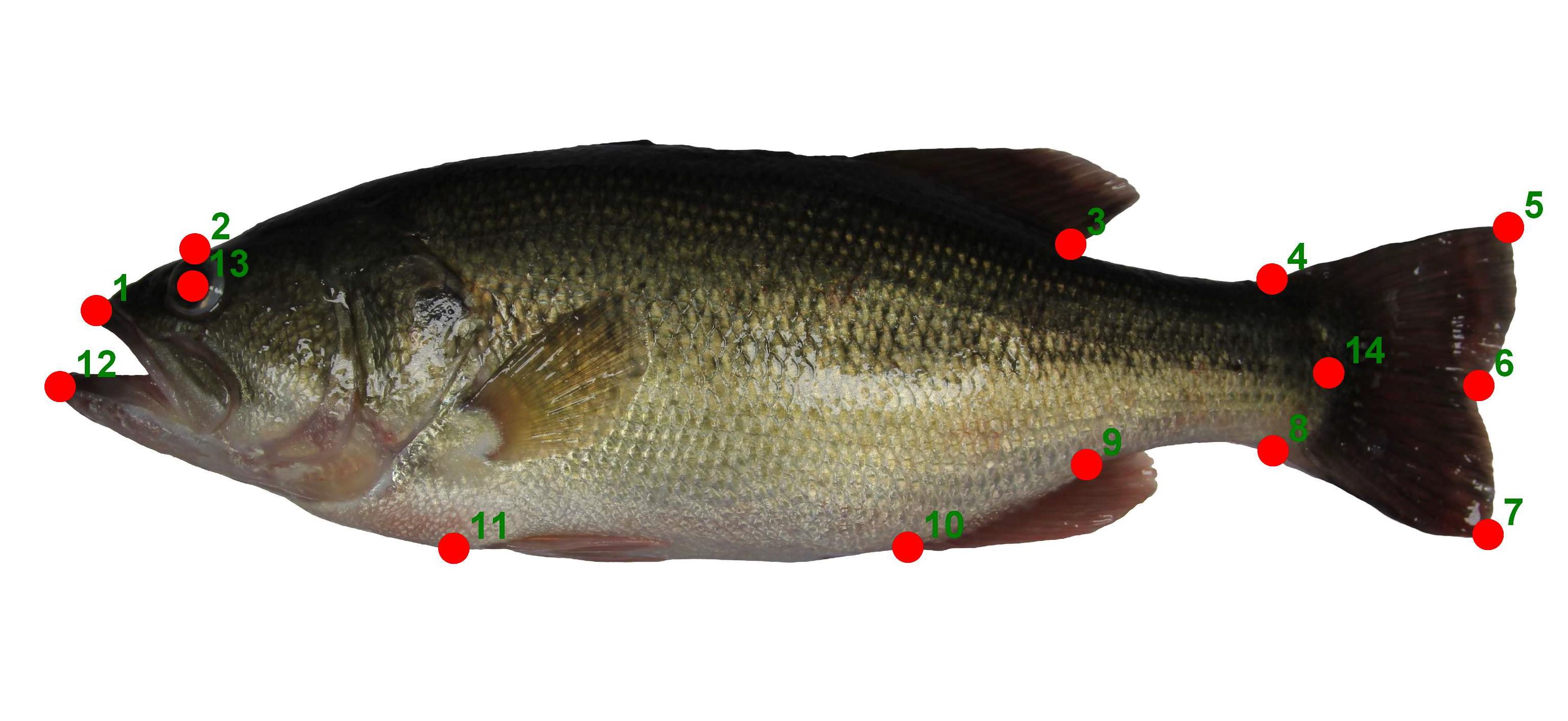
Figure 1. Landmarks placement of largemouth bass used in this study. The definition of landmarks depends on the biological interpretation specific to each research scope.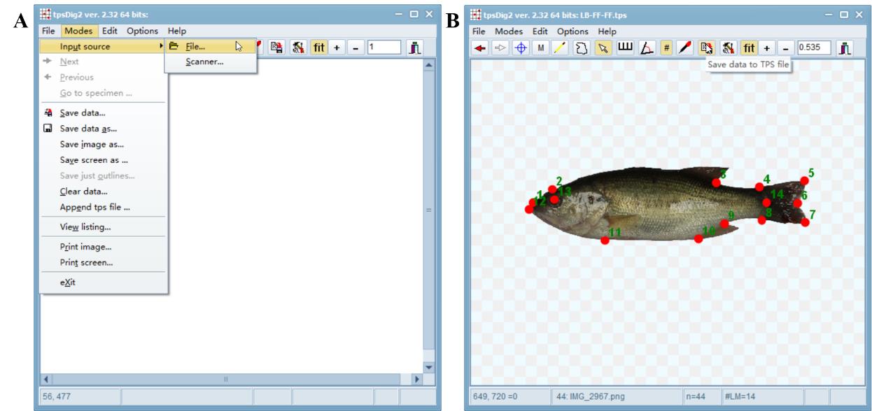
Figure 2. Process of landmark placing using software tpsDig2. A. Input source .tps file. B. Save data to .tps file after finishing landmarking.Set scale according to measurement methodology.
Scale image one by one
Open tpsDig2 → Image edit tools → Measure → Scale factor → Reference length (1-Centimeters) → Set scale → Draw a line with the same reference length → OK → Back to tpsDig2 window → Save data to TPS file → (LB-FF-FF.tps) → Save → Overwrite.
Scale as a variable for all images
Open tpsUtil → Operation → Add variable → Input file → Input → Click (LB-FF-FF.tps) and open → Output file → Name the output file with .tps as extensions (LB-FF-FF _allscale.tps) → Actions → Setup → Fill Variable keyword (Scale) → Fill Value → Create → Close.
Compile files (.tps)
If the images are not landmarked together with all the required data in one document, the .tps files should first be collected in one folder and then compiled into a single file by appending them.
Open tpsUtil → Operation → Append files → Input file → Input → Click (Group1.tps) and open → Output file → Name the output file with .tps as extensions (Expreiment1-Appendgroupfile.tps) → Actions → Setup → Tick .tps files → Create → Close.
The format of .tps file in GM
In GM, .tps files are commonly used to store landmark data. These files contain both landmark coordinates and additional information about the specimen. The .tps file format was first developed by Fred L. Bookstein in the 1990s. To check the contents of a .tps file, you can open it as a .txt document.
The general format of a TPS file is as follows:
LM= 14
19.00000 170.00000
81.00000 206.00000
616.00000 217.00000
…
774.00000 155.00000
IMAGE= F:\Directory\Images\ LB-FF-FF \IMG_2852.jpg
ID=0
VARIABLES=Scale=0.018155
…
A .tps file consists of two parts: a header (LM = 14) and a data section. The header provides information about the number of landmarks, while the data section contains the actual landmark coordinates. Each line in the data section represents a single landmark with its x-coordinate and y-coordinate. Additionally, other information such as image ID, image directory, specimen ID, and scale can be included at the beginning or end of each specimen's data.
Convert .tps format file to .nts format for use in MorphoJ
Open tpsUtil → Operation → Convert tps/nts coordinates file → Input file → Input → Click (LB-FF-FF_allscale.tps) and open → Output file → Name the output file with .nts as extensions (LB-FF-FF_allscale.nts) → Actions → Create → (Tick “use scale factor” [this will convert the pixel coordinates into standard units of measurements], 2D landmarks and Image name) → Create → Close.
The format of .nts file in GM
The .nts (Numerical Taxonomic System) file format is a legacy format used for storing landmark data, developed by Fred Bookstein in the early 1980s. .nts files can be created and edited using various software programs, including MorphoJ, tpsDig, and tpsRelw.
The general format of a .nts file is as follows:
1 44L 28L 0
IMG_2852.jpg IMG_2854.jpg…IMG_2976.jpg
X1 Y1 X2 Y2…X14 Y14
176.00000 384.00000 223.00000 419.00000 … 854.00000 376.00000
…
The parameters in the .nts file must adhere to specific guidelines. The first code in the parameter line should be "1". The second parameter, 44L, denotes the number of specimens, while the third parameter, 28L, represents the total count of x and y coordinates for each specimen. The fourth code in the parameter line is "0,” indicating the absence of missing data; if missing data exists, this code should be "1." It's important to note that some editing or removing redundant blank spaces may be necessary if a file does not solely consist of a single data matrix.
Shape variation analysis and visualization with MorphoJ
Create project and dataset [24]
File → New Project → Name for the new project (Project-images1) → Dimensionality of the data (2 dimensions) → Object symmetry? (no) → Name for the new dataset (Dataset- LB-FF-FF) → File type (NTSYSpc) → Add documents (LB-FF-FF_allscale.nts) → Create Dataset (Figure 3A) → File → Save Project → Name the Project (Project-LMB1.morphoj)
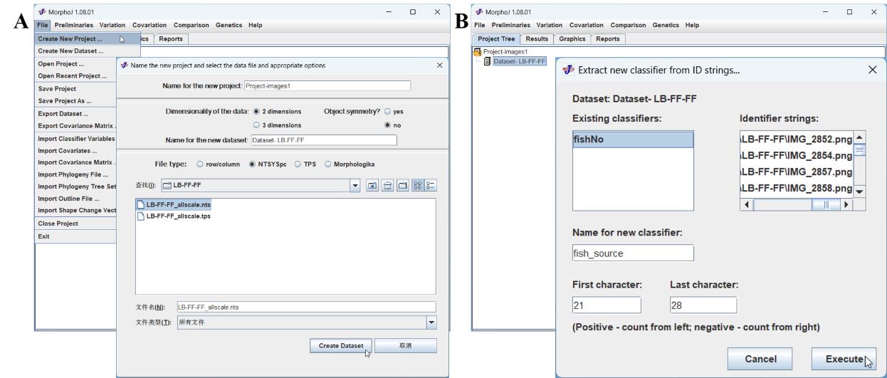
Figure 3. Creating a project and extracting a classifier in MorphoJ software. A. Creating a project and dataset. B. Extracting the classifier from ID strings by counting positively from left to right.Extract and add classifiers
Preliminaries → Extract new classifier from ID strings → Name for a new classifier (fish_source) → First character (21) → Last character (28) → Execute (Figure 3B).
Repeat the above steps to add more classifiers and the added classifiers can be edited from: Preliminaries → Edit classifiers (or directly click Graphics).
Outliers check
Preliminaries → Find outliers.
Repeat the above steps to create other datasets
Procrustes fit
MorphoJ uses a full Procrustes fit. For most circumstances, there is very little difference from generalized Procrustes analysis (GPA).
Preliminaries → New Procrustes Fit → Select Align by principal axes → Perform Procrustes Fit.
Export dataset for use in other software
Project Tree → Click Dataset (Dataset-images1.NTS) (Dataset-LB-FF-FF) → Click File in menu → Export Dataset → Select Data types and Classifiers (click with Ctrl or Shift for more than one type) → Name the Dataset as .txt file (Dataset-images1.NTS.txt) → Save.
Principal component analysis (PCA)
Purpose: Reduces the dimensionality of the shape data and identifies the main axes of variation.
Output: Principal components (PCs) that describe the major patterns of shape variation, and scatter plots of specimens in PC space.
Preliminaries → Generate Covariance Matrix → Selected dataset (Dataset-images1.NTS) → Execute → Variation → PCA → Results (without ticking the box “Pooled within-group covariances.”).
Eigenvalues → Variance explained by each PC.
PC scores → Visualization of individuals in the shape space.
Combine datasets
Click on the dataset in the Project Tree → Preliminaries → Combine Datasets → Name for the new dataset → Select the Start dataset and other datasets → Execute.
Discriminant function analysis (DFA)
Purpose: Classifies specimens into predefined groups based on shape.
Output: Discriminant functions, classification accuracy, scatter plots of specimens in discriminant space.
Click on the combined dataset → Comparison menu → Discriminant Function → Name for the discriminant function analysis → Select Dataset and Datatype (combined dataset) → Classifier to be used as grouping criterion (fish_source) → Select Pairs of groups to be included (or tick “Include all pairs of groups”) → Permutation runs:1000 → Execute.
Canonical variate analysis (CVA)
Purpose: Maximizes separation between predefined groups (e.g., species, populations) to find axes that best differentiate the groups.
Output: Canonical variates (CVs), scatter plots showing group separation (Figure 4), classification rates.
Click the combined dataset → Comparison menu → Canonical Variate Analysis → Name the CVA → Select the Dataset and Data type → Select classifier variable to use for grouping (fish_source) → Tick Permutation tests → Number of iterations = 10,000 → Execute.
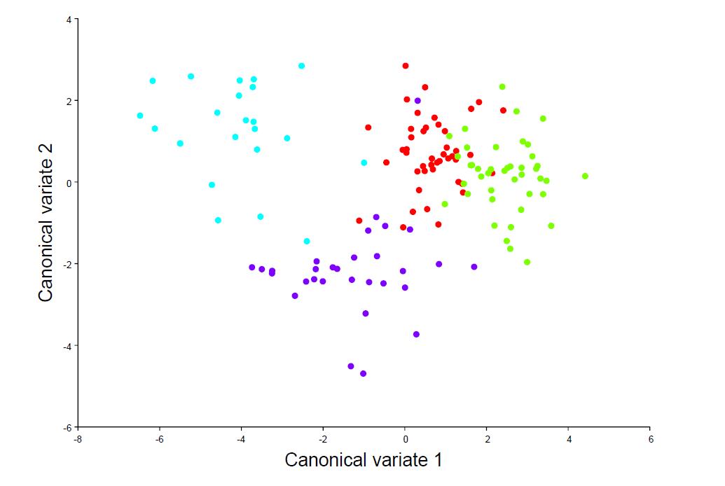
Figure 4. Scatterplot of the CV scores showing the shape features that best distinguish multiple groups of specimens. The color of points represents different specimen groups.Visualization of DFA shape difference combined with outline data
Extract fish outline
Open ImageJ → File → Open → Select the background removed image → Open → Image → 8-bt → Image → Adjust → Brightness/Contrast (Figure 5A) → Adjust the minimum and maximum value → Apply → Apply Lookup Table → OK → Process → Binary → Make Binary → Process → Binary → Fill holes → Process → Binary → Outline → Wand (tracing) tool → Click the outline of the fish → File → Save As → Jpeg → Save.
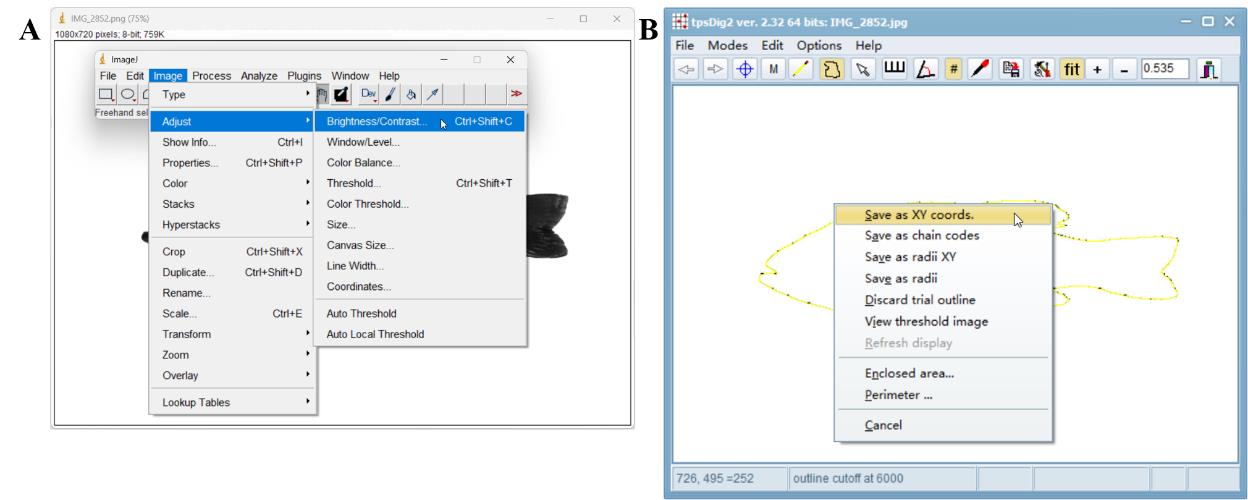
Figure 5. Extracting an outline and creating an outline file for use in MorphoJ software. A. Adjusting brightness and contrast while extracting the outline using ImageJ software. B. Creating the outline file through the outline object tool and saving it as xy coordinates using tpsDig2 software.Create outline file.
Open tpsDIG2 → File → Input source → File → Select the outline image → Open → Outline object → Right click to save as “Save as XY coords.” (Figure 5B) → File → Save just outlines → Save the outline as .txt files → Copy the coords. to Excel or other table processing software → Insert landmarks before the coodrs. → Insert a column to number the landmarks and coords. (such as “0” and “1,” respectively) → Copy the data back to .txt file to create a file.
Import outline file.
Click the dataset → File → Import Outline File → Name for the outline → Select the outline file → Open → Jump to Graphics of DFA → Shape difference → Right click → Change the type of graph → Warped Outline Drawing (Figure 6).
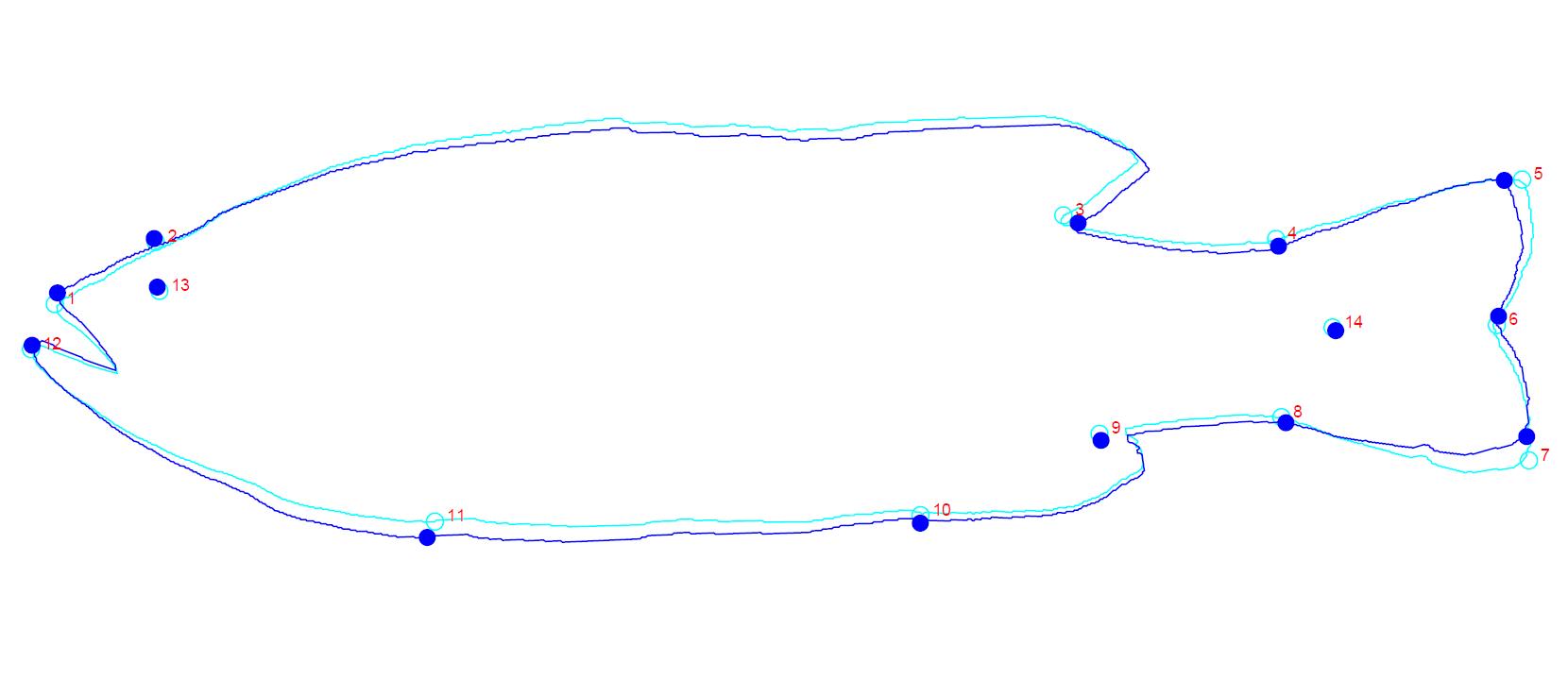
Figure 6. Visualization of discriminant function analysis (DFA) shape difference. Combining with outline data, the shape differences show general changes from the first to the second group. Lollipop graph and transformation grid graph can also be used to display specific variations.
Outline analysis and visualization with the Momocs R package
The analysis of semi-landmark data follows a procedure similar to that previously described. The outlined data analysis is subjected to the following steps using the Momocs R package [25].
### Starting
setwd("F:/Directory/GM-momocsu/IMGS") # Working directory
library(Momocs)
### Collection of outline coordinates data
## Extract outline coordinates from image files
lf1 <- list.files('F:/Directory/GM-momocsu/IMGS/LB-FF-FF-FIJI', full.names = TRUE)
lf1
coo1 <- import_jpg(lf1) # Data storage directory/Coo1
## Export each outline coordinates as a .csv file
# For coo1: Data storage directory/Coo1
setwd("F:/Directory/GM-momocsu/IMGS/outputdata/coo1_ff")
coo_list <- lapply(1:length(coo1), function(i) {
df <- data.frame(
x = coo1[[i]][, 1],
y = coo1[[i]][, 2],
image = basename(lf1[i])
)
return(df)
})
#
for (i in seq_along(coo_list)) {
filename <- paste0("outline_", i, ".csv")
write.csv(coo_list[[i]], file = filename, row.names = FALSE)
}
#
## Import and combine individual data files
library(dplyr)
imported_files1 <- lapply(paste0("outline_", seq_len(length(lf1)), ".csv"), read.csv)
combined_df1 <- bind_rows(imported_files1)
## Export as a combined .csv file
write.csv(combined_df1, file = "combined_outlines1.csv", row.names = FALSE) # (Supplemental File 2. combined_outlines1.csv).
### Loading data, converting to an Out object and inspecting
setwd("F:/Directory/GM-momocsu/IMGS/outputdata/coo1_ff")
## Read the .csv file
coo1_ff <- read.csv("combined_outlines1.csv")
# Convert the data frame to a list of matrices
coo1_list <- lapply(split(coo1_ff[, c("x", "y")], coo1_ff$image), as.matrix)
## Convert the list of matrices to an Out object
out1 <- Out(coo1_list)
## Plots outlines for inspection
# Panels of outlines (Figure 7)
panel(out1, c(6, 8),names=TRUE, cex.names=0.5)
# Plot one of the Out
coo_plot(out1[3])
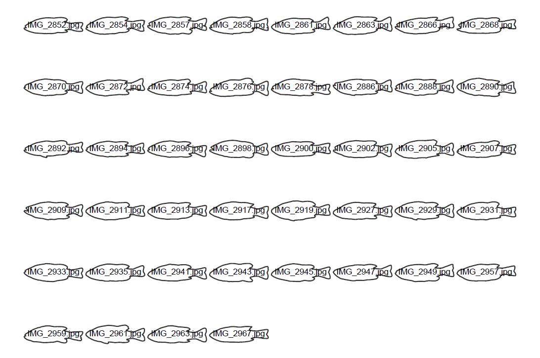
Figure 7. Outlines of largemouth bass from one experimental group. The panel of outlines can be used for inspecting the extraction.## Check if the outline is closed
coo_is_closed(out1)
### Outline data normalization
## Outline smoothing
# Extract coordinates from the Out object
coo_list_out1 <- lapply(out1$coo, function(coo) as.matrix(coo))
# Apply smoothing to each set of coordinates
smoothed_coo_list_out1 <- lapply(coo_list_out1, function(coo) coo_smooth(coo, n = 5))
# Convert the smoothed coordinates back to an Out object
smoothed_out1 <- Out(smoothed_coo_list_out1)
# Check for one of the smoothed outline
coo_plot(smoothed_out1[2], main = "iterations=5")
## Centering and scaling the outlines
# Center each set of coordinates
centered_matrices_out1 <- lapply(coo_list_out1, coo_center)
# Scale each set of coordinates
scaled_matrices_out1 <- lapply(centered_matrices_out1, coo_scale, scale = 1)
# Reconstruct the Out object
centered_scaled_out1 <- Out(scaled_matrices_out1)
# Check for centering and scaling
stack(centered_scaled_out1)
## Sampling pseudo-landmarks and reversing anticlockwise coordinates
# Sampling pseudo-landmarks
out1_resample <- coo_sample(centered_scaled_out1, 1000)
# Test if all shapes are developing consistently clockwise
coo_likely_clockwise(out1_resample)
# If not, the coordinates can be reversed
out1_resample_rev <- out1_resample
# Prepare Coo data for reversing
out1_rev_coo <- out1_resample_rev$coo
# Iterate over each outline
for (i in seq_along(out1_rev_coo)) {
# Extract the coordinates for this outline
coords <- out1_rev_coo[[i]]
# Check if the outline is likely not clockwise
if (!coo_likely_clockwise(coords)) {
# Reverse the coordinates
reversed_coords <- coo_rev(coords)
# Update the outline within the list
out1_rev_coo[[i]] <- reversed_coords
}
}
#
# Check if all outlines are clockwise
out1_rev_coor <- Out(out1_rev_coo)
coo_likely_clockwise(out1_rev_coor) # All TRUE
### Adjust data by defining landmarks, sliding coordinates to create Coe objects
## Define landmarks on the sampled-reversed outlines
out1_rev_coor_ldk <- def_ldk(out1_rev_coor,4)
## Sliding coordinates
out1_rev_coor_ldks <- coo_slide(out1_rev_coor_ldk,ldk = 1)
## Procrustes superimposition
out1_rev_coor_ldks_fgp <- fgProcrustes(out1_rev_coor_ldks)
## Creation Coe objects by Elliptical Fourier transform
out1_rev_coor_ldks_fgp_ef <- efourier(out1_rev_coor_ldks_fgp, 12, norm = FALSE) # In some cases, Elliptical Fourier Transform may address the limitations of traditional methods [26].
### Principal component analysis (PCA) and successive statistics
## PCA for the group out1
out1_rev_coor_ldks_fgp_ef_pca <- PCA(out1_rev_coor_ldks_fgp_ef)
summary(out1_rev_coor_ldks_fgp_ef_pca)
boxplot(out1_rev_coor_ldks_fgp_ef_pca, fac = NULL, nax = 1:12)
scree_plot(out1_rev_coor_ldks_fgp_ef_pca)
## For PCA of combined outlines
# Repeating the previous steps to develop data for other groups
# Combining group outlines
outall_rev_coor_ldks_fgp <-combine(out1_rev_coor_ldks_fgp,
out2_rev_coor_ldks_fgp,
out3_rev_coor_ldks_fgp,
out4_rev_coor_ldks_fgp)
# Creating Coe objects
outall_rev_coor_ldks_fgp_ef <- efourier(outall_rev_coor_ldks_fgp, 12, norm = FALSE)
# PCA and visualization
outall_rev_coor_ldks_fgp_ef_pca <- PCA(outall_rev_coor_ldks_fgp_ef)
summary(outall_rev_coor_ldks_fgp_ef_pca)
boxplot(outall_rev_coor_ldks_fgp_ef_pca, fac = NULL, nax = 1:12)
scree_plot(outall_rev_coor_ldks_fgp_ef_pca) # (Figure 8)
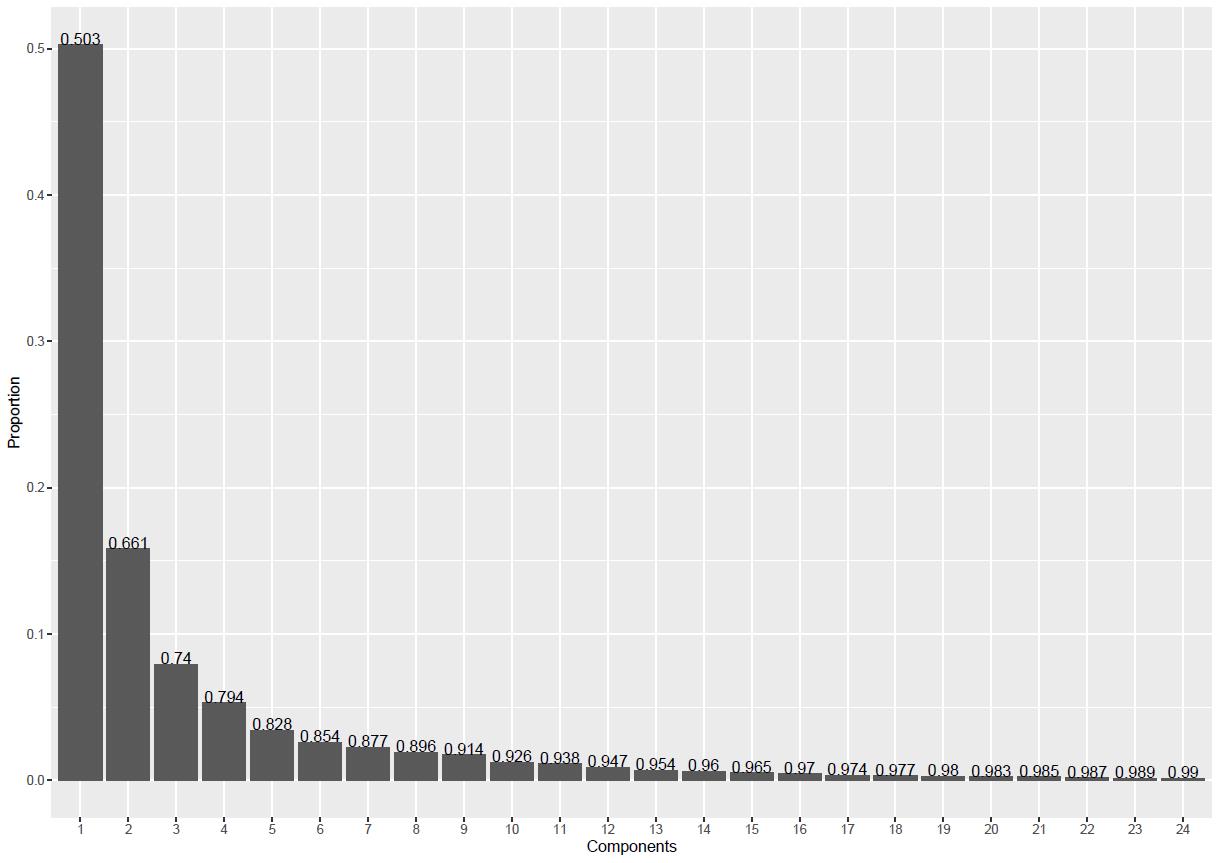
Figure 8. Principal component analysis (PCA) shows the proportion of each component for combined outlines. The number on top of each column of the bar chart represents the accumulated proportion of the 24 components.
### Mean shape analysis and Thin plate spline (TPS) analysis
## Mean shape analysis and visualization
out1_rev_coor_ldk_fgps_ef_mean <- (MSHAPES((out1_rev_coor_ldk_fgps_ef), fac = NULL, FUN = mean, nb.pts = 1000))
# Visualization of mean shape
coo_plot(out1_rev_coor_ldk_fgps_ef_mean)
# Visualization of mean shape and group outlines (Figure 9)
out1_rev_coor_ldks_fgp %>% coo_center %>% stack
coo_draw(out1_rev_coor_ldks_fgp_ef_mean,border='forestgreen',lwd = 3)
# Visualization of mean shapes differences
coo_arrows(out1_rev_coor_ldks_fgp_ef_mean,
out2_rev_coor_ldks_fgp_ef_mean,length = coo_centsize(out1_c)/2, angle = 20, code = 2)
coo_draw(out2_rev_coor_ldks_fgp_ef_mean, border = "blue", centroid = T,
first.point = F, zoom = 0.7, lwd = 2)
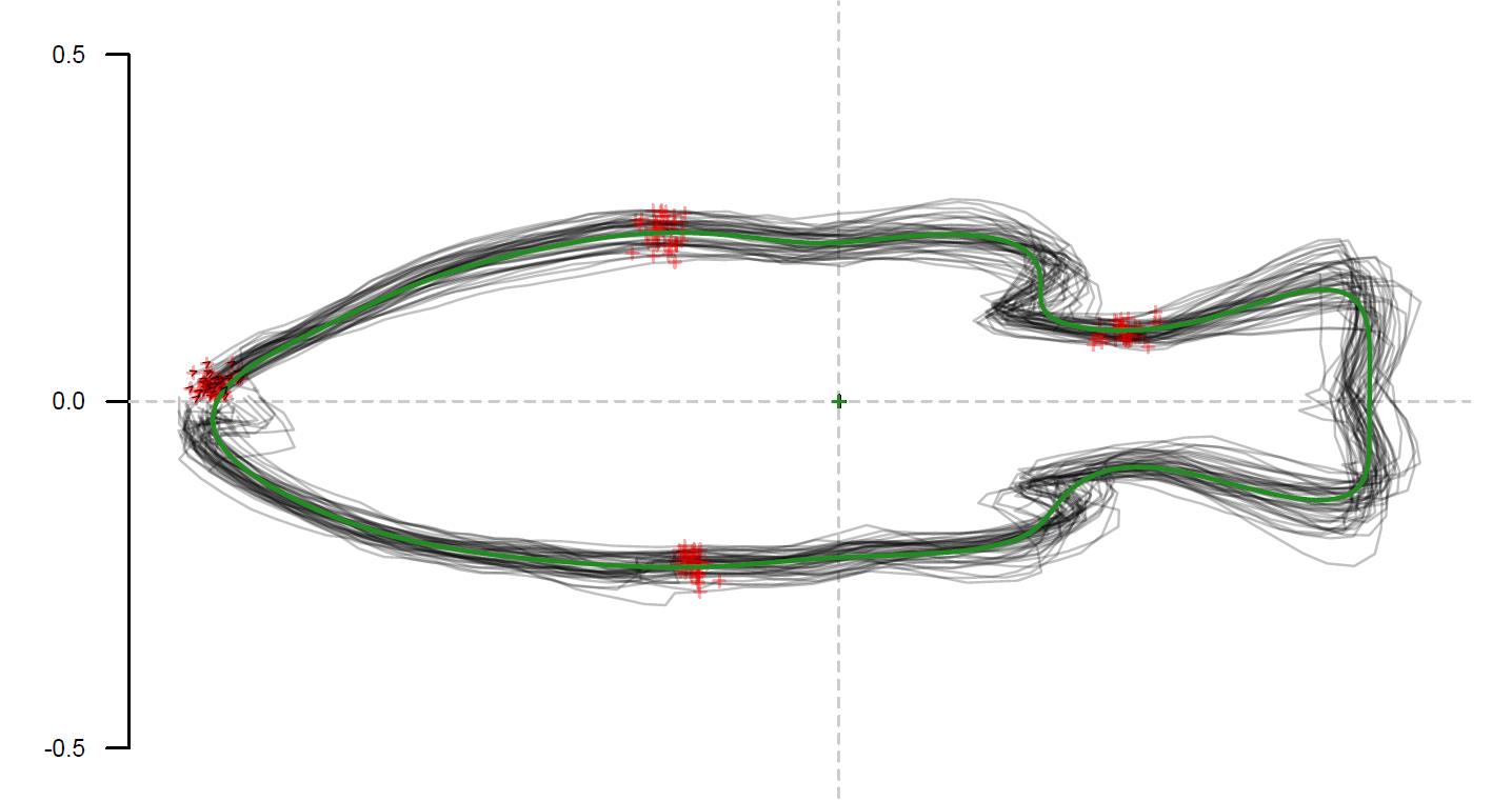
Figure 9. Visualization of the mean shape and stacked outlines from the experimental Group 1. The green line represents the mean shape of the outlines from Group 1, while the grey lines represent the individual outlines from Group 1.## Thin plate spline analysis (TPS) (Figure 10)
tps_grid(out1_rev_coor_ldks_fgp_ef_mean,
out3_rev_coor_ldks_fgp_ef_mean, over = 1.2,amp=1, grid.size=20,shp.border = c("red", "blue"),
shp.lwd = c(2, 2),legend = F)
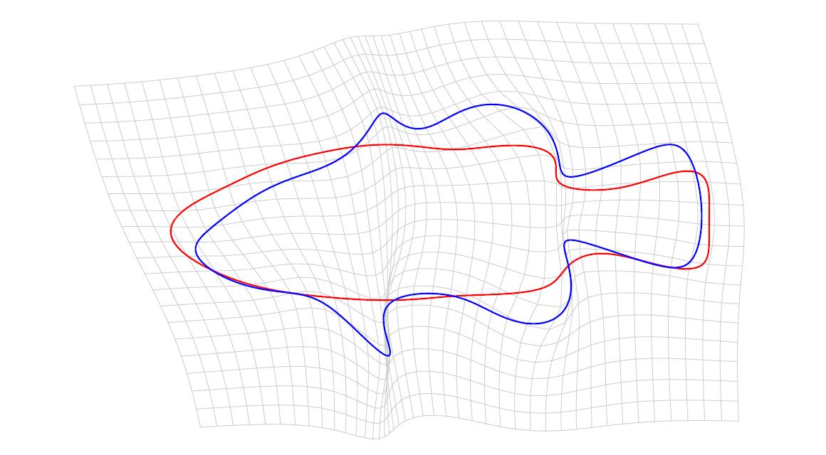
Figure 10. Visualization of the mean shape difference between experimental Group 1 and Group 3 through thin plate spline (TPS) analysis. The red line represents the mean shape of outlines for Group 1, while the blue line represents the mean shape of outlines for Group 3.
Validation of protocol
This protocol or parts of it has been used and validated in the following research articles:
Santos et al. [27]. Geometric morphometrics as a tool to identify species in multispecific flatfish landings in the Tropical Southwestern Atlantic. Fish Res. (Figure 2, 3).
Caillon et al. [28]. A morphometric dive into fish diversity. Ecosphere. (Figure 1, 3).
Rabe et al. [29]. Geometric morphometric analysis of an ontogenetic cranial series of the Permian dicynodont Diictodon feliceps. Proc R Soc B. (Figure 2).
General notes and troubleshooting
Based on experience from the current research, the size of an image used for outline extraction should be no smaller than 14 KB.
For research requiring scale, landmarking should be performed for measurements before removing the image background.
If a landmark is misplaced, all subsequent landmarks in that image must be crossed out. The researcher needs to correct the misplacement by re-establishing the landmarks from scratch.
For images of fish without an original scale, real measurements cannot be accomplished. In the methods section for setting the scale for measurement, the scale can be set to “scale=1.”
Based on the current versions of tpsDig2 (Version 2.32) and tpsUtil (Version 1.82), the file path is included in the name of each image during the process of creating the .tps file and placing landmarks. Sometimes, the image name in the .tps file may be presented as its original name. Therefore, prior to landmarking, images from each group should be appropriately named to differentiate them from one another and to provide sufficient information regarding their biological characteristics. For example, the images can be named LB_Foshan_group1_female_mature_bait1_IMG_1001.jpeg. The names can be shortened as necessary by abbreviating words within the name.
The xy coordinates of the outline can also be created using ImageJ software, though the number of coordinates is typically much less than that generated through tpsDig2.
For outline analysis, reversing the anticlockwise coordinates and defining landmarks to create Coe objects are two key steps for samples with significant shape variations among images in a group.
When applying this protocol to GM analyses in other species, landmarking, outline extraction, and the selection of analysis methods should correlate with biological interpretation.
Acknowledgments
The author thanks Dr. Tingwei Zhang for assisting in taking photos of fish. This work was supported by the Central Public-interest Scientific Institution Basal Research Fund, CAFS (2024SJRC9), the Project of Innovation Team of Survey and Assessment of the Pearl River Fishery Resources (2023TD10) and the National Natural Science Foundation of China (31600446).
Competing interests
The author declares no competing interests.
Ethical considerations
All animal study protocols were approved by the Laboratory Animal Ethics Committee of Pearl River Fisheries Research Institute, CAFS (LAEC-PRFRI-20160323).
References
- Polly, P. D. and Motz, G. J. (2016). PATTERNS AND PROCESSES IN MORPHOSPACE: GEOMETRIC MORPHOMETRICS OF THREE-DIMENSIONAL OBJECTS. The Paleontological Society Papers 22: 71–99. https://doi.org/10.1017/scs.2017.9
- Dwivedi, A. K. and De, K. (2023). Role of Morphometrics in Fish Diversity Assessment: Status, Challenges and Future Prospects. Natl Acad Sci Lett. 47(2): 123–126. https://doi.org/10.1007/s40009-023-01323-x
- Lawing, A. M. and Polly, P. D. (2009). Geometric morphometrics: recent applications to the study of evolution and development. J Zool. 280(1): 1–7. https://doi.org/10.1111/j.1469-7998.2009.00620.x
- Collyer, M. L., Davis, M. A. and Adams, D. C. (2020). Making Heads or Tails of Combined Landmark Configurations in Geometric Morphometric Data. Evol Biol. 47(3): 193–205. https://doi.org/10.1007/s11692-020-09503-z
- Palmqvist, P. (2022). Recensión. Fred L. Bookstein, 1991. Morphometric Tools for Landmark Data: Geometry and Biology. Cambridge University Press, Cambridge. ISBN 0-521-38385-4. Span J Palaeontol. 7(2): 166. https://doi.org/10.7203/sjp.25045
- Bookstein, F. L. (2018). Geometric morphometrics: its geometry and its pattern analysis, in: Bookstein, F.L. (Ed.), A Course in Morphometrics for Biologists. Cambridge University Press, Cambridge, pp. 322–493. https://doi.org/10.1017/9781108120418.006
- Wärmländer, S. K. T. S., Garvin, H., Guyomarc'h, P., Petaros, A. and Sholts, S. B. (2018). Landmark Typology in Applied Morphometrics Studies: What's the Point?. Anat Rec. 302(7): 1144–1153. https://doi.org/10.1002/ar.24005
- Webster, M. and Sheets, H. D. (2010). A Practical Introduction to Landmark-Based Geometric Morphometrics. In Alroy, J., Hunt, G. (Eds.), Quantitative methods in Paleobiology. Cambridge University Press, Cambridge, pp. 16: 163–188. https://doi.org/10.1017/s1089332600001868
- Thompson, D. A. (1917). On growth and form. Abridged and edited by j. T. Bonner, Cambridge University Press, 1961. Cambridge University Press, Cambridge.
- Bookstein, F. L. (2024). Quadratic Trends: A Morphometric Tool Both Old and New. Evol Biol. 51(1): 1–44. https://doi.org/10.1007/s11692-023-09621-4
- Bookstein, F. L. (2023). Reworking Geometric Morphometrics into a Methodology of Transformation Grids. Evol Biol. 50(3): 275–299. https://doi.org/10.1007/s11692-023-09607-2
- Hu, H., Bjarnason, A. and Benson, R. (2021). 3D geometric morphometric protocol - quantifying the morphology of living and extinct vertebrates. Bio-101: e1010664. https://doi.org/10.21769/BioProtoc.1010664
- Wang, C., Fang, Z. and Chen, X. J. (2022). Advances in the application of biometrics-based geometric morphometrics in fisheries. Marine Fisheries. 44 (1): 112–128. https://doi.org/10.13233/j.cnki.mar.fish.2022.01.004
- Tong, Y., Zhang, M., Jenkins Shaw, J., Wan, X., Yang, X., Bai, M. (2021). A geometric morphometric dataset of stag beetles. Biodivers Sci. 29(9): 1159–1164. https://doi.org/10.17520/biods.2021160
- Moccetti, P., Rodger, J. R., Bolland, J. D., Kaiser-Wilks, P., Smith, R., Nunn, A. D., Adams, C. E., Bright, J. A., Honkanen, H. M., Lothian, A. J., et al. (2023). Is shape in the eye of the beholder? Assessing landmarking error in geometric morphometric analyses on live fish. PeerJ. 11: e15545. https://doi.org/10.7717/peerj.15545
- Schneider, C. A., Rasband, W. S. and Eliceiri, K. W. (2012). NIH Image to ImageJ: 25 years of image analysis. Nat Methods. 9(7): 671–675. https://doi.org/10.1038/nmeth.2089
- Rohlf, F. J. (2021). https://sbmorphometrics.org/index.html [Accessed January 31, 2023]
- Klingenberg, C. P. (2010). MorphoJ: an integrated software package for geometric morphometrics. Mol Ecol Resour. 11(2): 353–357. https://doi.org/10.1111/j.1755-0998.2010.02924.x
- R Core Team (2023). R: A Language and Environment for Statistical Computing. R Foundation for Statistical Computing, Vienna, Austria. https://www.R-project.org. [Accessed October 31, 2023]
- Posit team. (2023). RStudio: Integrated Development Environment for R. Posit Software, PBC, Boston, MA. URL http://www.posit.co/. [Accessed October 31, 2023]
- Karki, N. P., Colombo, R. E., Gaines, K. F. and Maia, A. (2020). Exposure to 17β estradiol causes erosion of sexual dimorphism in Bluegill (Lepomis macrochirus). Environ Sci Pollut Res. 28(6): 6450–6458. https://doi.org/10.1007/s11356-020-10935-5
- Elmer, K. R., Kusche, H., Lehtonen, T. K. and Meyer, A. (2010). Local variation and parallel evolution: morphological and genetic diversity across a species complex of neotropical crater lake cichlid fishes. Philos Trans R Soc Lond B Biol Sci. 365(1547): 1763–1782. https://doi.org/10.1098/rstb.2009.0271
- Savriama, Y. (2018). A Step-by-Step Guide for Geometric Morphometrics of Floral Symmetry. Front Plant Sci. 9: e01433. https://doi.org/10.3389/fpls.2018.01433
- Crampton, D. A., Giacomini, G. and Meloro, C. (2024). Mandibular morphology in four species of insectivorous bats: the impact of sexual dimorphism and geographical differentiation. J Zool. 323(4): 331–345. https://doi.org/10.1111/jzo.13177
- Bonhomme, V., Picq, S., Gaucherel, C. and Claude, J. (2014). Momocs: Outline Analysis UsingR. J Stat Softw. 56(13): ei13. https://doi.org/10.18637/jss.v056.i13
- García-Bustos, M., García Bustos, P. and Rivero, O. (2024). New Methods for Old Questions: The Use of Elliptic Fourier Analysis for the Formal Study of Palaeolithic Art. J Archaeol Method Theory. https://doi.org/10.1007/s10816-024-09656-7
- Santos, S. R., Pessôa, L. M. and Vianna, M. (2019). Geometric morphometrics as a tool to identify species in multispecific flatfish landings in the Tropical Southwestern Atlantic. Fish Res. 213: 190–195. https://doi.org/10.1016/j.fishres.2019.01.017
- Caillon, F., Bonhomme, V., Möllmann, C. and Frelat, R. (2018). A morphometric dive into fish diversity. Ecosphere 9(5): e2220. https://doi.org/10.1002/ecs2.2220
- Rabe, C., Marugán-Lobón, J., Smith, R. M. H. and Chinsamy, A. (2024). Geometric morphometric analysis of an ontogenetic cranial series of the Permian dicynodont Diictodon feliceps. Proc R Soc B. 291(2027): e0626. https://doi.org/10.1098/rspb.2024.0626
Supplementary information
The following supporting information can be downloaded here:
- Supplemental File 1. LB-FF-FF.tps
- Supplemental File 2. combined_outlines1.csv
Article Information
Publication history
Received: Jun 12, 2024
Accepted: Aug 25, 2024
Available online: Sep 13, 2024
Published: Oct 20, 2024
Copyright
© 2024 The Author(s); This is an open access article under the CC BY-NC license (https://creativecommons.org/licenses/by-nc/4.0/).
How to cite
Luo, D. (2024). Quantitative Analysis of Fish Morphology Through Landmark and Outline-based Geometric Morphometrics with Free Software. Bio-protocol 14(20): e5087. DOI: 10.21769/BioProtoc.5087.
Category
Bioinformatics and Computational Biology
Biological Sciences > Biological techniques
Environmental science > Marine vertebrates
Do you have any questions about this protocol?
Post your question to gather feedback from the community. We will also invite the authors of this article to respond.