
- Submit a Protocol
- Receive Our Alerts
- EN

- Protocols

- Articles and Issues
- For Authors
- About
- Become a Reviewer

GATK Variant Discovery Pipeline
Published: Sep 20, 2024 DOI: 10.21769/BioProtoc.5068 Views: 157
Reviewed by: Anonymous reviewer(s)

Protocol Collections
Comprehensive collections of detailed, peer-reviewed protocols focusing on specific topics


Abstract
Phenotypic variations of most biological traits are largely driven by genomic variants. The single nucleotide polymorphism (SNP) is the most common form of genomic variants. Multiple algorithms have been developed for discovering genomic variants, including SNPs, with next-generation sequencing (NGS) data. Here, we present a widely used variant discovery pipeline based on the software Genome Analysis ToolKits (GATK). The pipeline uses whole-genome sequencing (WGS) data as input and includes read mapping, variant calling, and the variant filtering process. This pipeline has been successfully applied to many genomic projects and represents a solution for variant calling using NGS data.
Keywords: Variant discoveryGraphical overview
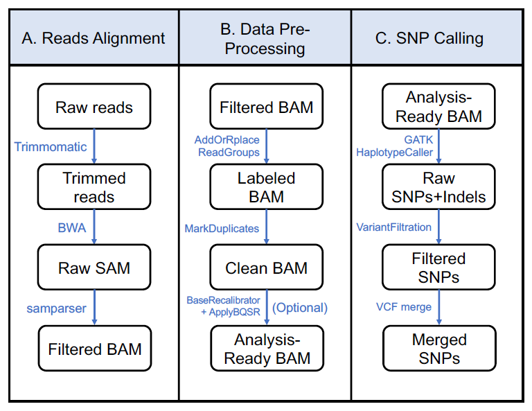 Workflow of the single nucleotide polymorphism (SNP) calling pipeline using GATK software
Background
As the technology allows regularly producing sequencing data in a high-throughput manner, genome-wide variant discovery becomes routine for many applications, including genotyping of variants for their phenotypic connection. Single nucleotide polymorphisms (SNPs) and small insertion–deletions (indels) are two common forms of genomic variants. The SNP, as the simplest molecular marker, has been widely used to connect genetic variation with phenotypic variation of biological traits, such as human diseases and plant architectures [1,2]. The reference-based SNP calling is the process by which DNA polymorphisms between sequencing reads and the reference are identified based on their alignments [3]. Algorithms and software packages have been developed for SNP calling. Simple SNP calling methods determine read counts at each polymorphic site and set a cutoff of read counts for SNP identification [4]. However, the power of SNP discovery using such methods is subject to sequencing depths. More sophisticated approaches incorporate the uncertainty of SNP calling in a probabilistic framework, such as SOAP2, SAMtools, or Genome Analysis ToolKits (GATK) [5–7]. Among them, GATK is the industry standard for discovering SNPs and small indels using sequencing data from genomic DNA and RNA-seq [7]. Although GATK was originally developed for human sequencing data, it has evolved to handle genome data from other organisms with different levels of ploidy [8]. Here, we present a variant calling pipeline using whole-genome sequencing (WGS) data based on GATK. The pipeline includes reads mapping, variant calling, and variant filtering.
Software and datasets
Software installation and data availability: All software installation instructions and test data have been deposited to GitHub: https://github.com/Bio-protocol/GATK-SNP-Calling
Software
All software packages have been tested on a Linux (CentOS 7, x86_64) operating system.
Anaconda (version 2024.02-1) (https://www.anaconda.com/download)
Trimmomatic (version 0.39, Java 1.8.0+) (http://www.usadellab.org/cms/?page=trimmomatic)
BWA (version 0.7.17) (https://github.com/lh3/bwa)
SAMtools (version 1.9) (http://www.htslib.org/)
GATK4 (version 3.8, Java 1.8.0+) (https://gatk.broadinstitute.org/)
vcftools (version 0.1.16) (http://vcftools.sourceforge.net/)
Perl (version 5) (https://perl.org)
Python (version 3) (https://python.org)
Sample data for GATK SNP Calling workflow include:
B73/A188.R1/2.fq.gz: Paired-end whole genome sequencing reads for two test samples.
B73Ref4.fa: The maize B73 version4 reference genome.
TruSeq3-PE.fa: The adaptor sequences for reads trimming.
Sample reads and adaptor sequences were included in the “input” folder. The B73 version4 reference genome can be downloaded from MaizeGDB (https://download.maizegdb.org/Zm-B73-REFERENCE-GRAMENE-4.0/Zm-B73-REFERENCE-GRAMENE-4.0.fa.gz)
Procedure
You can download the GitHub repository with this command line:
git clone https://github.com/Bio-protocol/GATK-SNP-Calling.git
cd GATK-SNP-Calling
Step 0: Installation of required software
Note: Conda should be installed first and bioconda channel needs to be added into the conda configure with this command “conda config --add channels bioconda”.
Install the Anaconda and add it into ~/.bashrc.
wget https://repo.anaconda.com/archive/Anaconda3-2024.02-1-Linux-x86_64.sh
bash Anaconda3-2024.02-1-Linux-x86_64.sh
echo 'export PATH="~/anaconda3/bin:$PATH"' >> ~/.bashrc
source ~/.bashrc
All dependencies can be installed through the GATK_SNP.yaml file in the GitHub repository.
conda env create -f GATK_SNP.yamlconda activate GATK_SNP
Alternatively, the conda environment can be created by following scripts if GATK_SNP.yaml is not used.
conda create -n GATK_SNP python=3conda activate GATK_SNP
conda install -c bioconda trimmomatic
conda install -c bioconda bwa
conda install -c bioconda samtools
conda install -c bioconda gatk4
conda install -c bioconda vcftools
Step 1: Raw reads trimming
The Trimmomatic software is a flexible read trimming tool for Illumina NGS data [9]. It is widely used to remove low-quality reads and sequence adapters. As test inputs are paired-end reads, we use the paired-end mode for sequence trimming.
The code for raw reads trimming is as follows:
#!/bin/bash
## B73 reads trimming ##
trimmomatic PE \
./input/B73.R1.fq.gz ./input/B73.R2.fq.gz \
./cache/B73_trim.R1.fq.gz ./cache/B73_unpaired.R1.fq.gz \
./cache/B73_trim.R2.fq.gz ./cache/B73_unpaired.R2.fq.gz \
ILLUMINACLIP:./input/TruSeq3-PE.fa:3:20:10:1:true LEADING:3 TRAILING:3 SLIDINGWINDOW:4:13 MINLEN:40 2> ./cache/B73_trim.log
## A188 reads trimming ##
trimmomatic PE \
./input/A188.R1.fq.gz ./input/A188.R2.fq.gz \
./cache/A188_trim.R1.fq.gz ./cache/A188_unpaired.R1.fq.gz \
./cache/A188_trim.R2.fq.gz ./cache/A188_unpaired.R2.fq.gz \
ILLUMINACLIP:./input/TruSeq3-PE.fa:3:20:10:1:true LEADING:3 TRAILING:3 SLIDINGWINDOW:4:13 MINLEN:40 2> ./cache/A188_trim.log
For one-step running, you can simply run this script:
sh ./workflow/1_reads_trim.sh
Note:
(1) The Trimmomatic software should be run on a 1.8.0+ Java environment.
(2) If you want to trim data with your own adapter sequences, you should replace the adapter sequences in TruSeq3-PE.fa file with your own adapter sequences.
Step 2: BWA read alignment
BWA is a software package for mapping low-divergent sequences against a reference genome [10]. Here, we use BWA to map the remaining trimmed reads to the B73v4 reference genome.
BWA index for the reference genome
cd input
wget https://download.maizegdb.org/Zm-B73-REFERENCE-GRAMENE-4.0/Zm-B73-REFERENCE-GRAMENE-4.0.fa.gz
gunzip Zm-B73-REFERENCE-GRAMENE-4.0.fa.gz
mv Zm-B73-REFERENCE-GRAMENE-4.0.fa B73Ref4.fa
bwa index B73Ref4.fa
cd ../
BWA alignment
## BWA alignment ##
bwadb=./input/B73Ref4.fa
B73_R1=./cache/B73_trim.R1.fq.gz
B73_R2=./cache/B73_trim.R2.fq.gz
A188_R1=./cache/A188_trim.R1.fq.gz
A188_R2=./cache/A188_trim.R2.fq.gz
bwa mem -t 8 -R '@RG\tID:B73\tSM:B73' $bwadb $B73_R1 $B73_R2 > ./cache/B73.sam
bwa mem -t 8 -R '@RG\tID:A188\tSM:A188' $bwadb $A188_R1 $A188_R2 > ./cache/A188.sam
Adjustable parameters for BWA:-t INT: Number of threads
-R STR: Complete read group header line. “\t” can be used in STR and will be converted to a TAB in the output SAM. The read group ID will be attached to every read in the output. An example is “@RG\tID:foo\tSM:bar”.
Note: Most parameters of BWA were set as default here; you can find the information of all the parameters in the BWA manual reference (https://bio-bwa.sourceforge.net/bwa.shtml)
For one-step running of this step, you can simply run this script:
sh ./workflow/2_bwa_align.sh
Step 3: SAM filtering and compressing
In this step, raw alignments (SAM format) are filtered and sorted based on alignment coordinates on the reference genome.
SAM filtering
Here, we use a Perl script to filter BWA alignment results (SAM format).
## SAM filtering ##perl ./lib/samparser.bwa.pl -i ./cache/B73.sam -e 100 -m 3 100 --tail 5 100 --gap 0 --insert 100 800 1>./cache/B73.parse.sam 2>./cache/B73.parse.log
perl ./lib/samparser.bwa.pl -i ./cache/A188.sam -e 100 -m 3 100 --tail 5 100 --gap 0 --insert 100 800 1>./cache/A188.parse.sam 2>./cache/A188.parse.log
Adjustable parameters for samparser.bwa.pl are:--input|i: SAM file
--identical|e: minimum matched and identical base length, default = 30 bp
--mismatches|mm|m: two integers to specify the number of mismatches out of the number of basepairs of the matched region of reads; matched regions are not identical regions, and mismatch and indel could occur, e.g., --mm 2 36 represents ≤ 2 mismatches out of 36 bp
--tail: the maximum bp allowed at each side, two integers to specify the number of tails out of the number of basepairs of the reads, not including "N", e.g., --tail 3 75 represents ≤ 3 bp tails of 75 bp of reads without "N"
--gap: if a read is split, an internal gap (bp) is allowed, default = 5000 bp
--mappingscore: the minimum mapping score, default = 40
--insert: insert range, e.g., 100 600 (default)
--help: help information
Note: We expect the percentage of mapped reads to be ~70% for our example organism.
BAM sort & index
The bam files are required to be sorted and indexed before GATK SNP calling.
## BAM sort & index ##cd cache
samtools view -u B73.parse.sam | samtools sort -o B73.parse.sort.bam
samtools view -u A188.parse.sam | samtools sort -o A188.parse.sort.bam
samtools index B73.parse.sort.bam
samtools index A188.parse.sort.bam
rm *.sam
cd ../
For one-step running of this step, you can simply run this script:
sh ./workflow/3_SAM_filter.sh
Step 4: Data pre-processing for GATK SNP calling
Before GATK SNP calling, aligned reads need to be pre-processed to meet the GATK requirements.
(Optional) Add labels for alignment reads
In BWA alignment step, we have already set sample names/groups. If this is not added during the BWA alignment, the following step must be added to BAM alignments. The GATK module “AddOrReplaceReadGroups” can be used to add the sample name/group information.
## Add labels for inputs ##gatk AddOrReplaceReadGroups --java-options '-Xmx24g' \
-I ./cache/B73.parse.sort.bam \
-O ./cache/B73.RG.bam \
-LB A -PL illumina -PU A -SM B73 -ID B73
gatk AddOrReplaceReadGroups --java-options '-Xmx24g' \-I ./cache/A188.parse.sort.bam \
-O ./cache/A188.RG.bam \
-LB A -PL illumina -PU A -SM A188 -ID A188
Adjustable parameters for AddOrReplaceReadGroups:-LB: Read-Group library#
-PL: Read-Group platform#
-PU: Read-Group platform unit#
-SM: Read-Group sample name#
-ID: Read-Group ID#
(Optional) MarkDuplicates
The GATK package “MarkDuplicates” is used to mark duplicated reads occurring during sample preparation such as library construction using PCR. The MarkDuplicates tool works by comparing sequences in the five prime positions of both reads and read-pairs in a SAM/BAM file. A BARCODE_TAG option is available to facilitate duplicate marking using molecular barcodes. After duplicated reads are marked, the GATK tool can differentiate the primary and duplicated reads using an algorithm that ranks reads by using the sum of quality scores of each read, which can improve the accuracy of variant calling.
## MarkDuplicates ##
gatk MarkDuplicates --java-options '-Xmx24g' --REMOVE_DUPLICATES true \
-I ./cache/B73.RG.bam \
-M ./cache/B73.metrics.txt \
-O ./cache/B73.RG.RD.bam
gatk MarkDuplicates --java-options '-Xmx24g' --REMOVE_DUPLICATES true \
-I ./cache/A188.RG.bam
-M ./cache/A188.metrics.txt
-O ./cache/A188.RG.RD.bam
## BAM index ##
cd cache
samtools index B73.RG.RD.bam
samtools index A188.RG.RD.bam
cd ../
(Optional) Recalibrate base quality scores
BQSR stands for base quality score recalibration. Using this module, alignment scores can be recalibrated according to known genomic variation data to improve variation calling. In our test samples, this step was skipped. However, the script is provided here.
## Generates recalibration table for Base Quality Score Recalibration (BQSR) ##gatk BaseRecalibrator \
-I input.RG.RD.bam \
-R reference.fa \
--known-sites sites_of_variation.vcf \
--known-sites another/optional/setOfSitesToMask.vcf \
-O recal_data.table
## Apply base quality score recalibration ##
gatk ApplyBQSR \
-R reference.fa \
-I input.RG.RD.bam \
--bqsr-recal-file recalibration.table \
For one-step running of this step, you can simply run this script:
sh ./workflow/4_data_preprocess.sh
Note: GATK and 1.8.0+ Java environment are required for this step.
Step 5: GATK short variant calling
GATK is a collection of command-line tools for analyzing high-throughput sequencing data with a primary focus on variant discovery. Here, we focus on short variants and use the “HaplotypeCaller” module to call SNPs and indels relative to a reference genome.
Create a GATK index of the reference genome
## gatk index for reference genome ##
samtool faidx input/B73Ref4.fa
gatk CreateSequenceDictionary -R input/B73Ref4.fa -O input/B73Ref4.dict
GATK short variant calling
## GATK SNP Calling (2 samples together) ##
gatk HaplotypeCaller --java-options '-Xmx24g' -R input/B73Ref4.fa -I cache/B73.RG.RD.bam -I cache/A188.RG.RD.bam -O output/B73_A188.raw.0.vcf
Notes:(1) The GATK short variant calling step can identify both SNPs and short indels; here, we focus on SNPs and filter out indels (Step 6: SNP filtering).
(2) We use the default parameters of GATK HapotypeCaller for short variant calling.
(3) We suggest doing GATK short variant calling with all samples together. If there are too many samples to load at the same time, you can use a bam list file including all sample information instead. An example bam.list file can be found in /input/bam.list; the format of the bam list file consists of the bam file path for each row. The code is as follows:
## GATK Short Variant Calling (with bam list) ##gatk HaplotypeCaller --java-options '-Xmx24g' \
-R ./input/B73Ref4.fa \
-I ./input/bam.list \
-O ./output/B73_A188.raw.0.vcf
For one-step running of this step, you can simply run this script:sh ./workflow/5_GATK.sh
Step 6: SNP filtering
To remove indels and retain high-quality SNPs, GATK provides the script module for filtering variants [11].
Select bi-allelic SNPs
## select bi-allelic SNPs ##vcf=./output/B73_A188.raw.0.vcf
ref=./input/B73Ref4.fa
gatk SelectVariants -R $ref -V $vcf \
--restrict-alleles-to BIALLELIC -select-type SNP \
-O ./output/B73_A188.bi.1.vcf.gz &>./output/B73_A188.bi.log
Filtering variants
## Hard-filtering germline short variants ##
gatk VariantFiltration --java-options '-Xmx24g' \
-R $ref -V ./output/B73_A188.bi.1.vcf.gz \
--filter-expression "QD < 2.0 || MQ < 40.0 || FS > 60.0 || MQRankSum < -12.5 || ReadPosRankSum < -8.0 || SOR > 3.0" \
--filter-name "hard_filter" \
-O ./output/B73_A188.HF.2.vcf.gz
## Extract PASS SNPs ##
gatk SelectVariants --java-options '-Xmx24g' \
-R $ref -V ./output/B73_A188.HF.2.vcf.gz \
--exclude-filtered \
-O ./output/B73_A188.PASS.3.vcf.gz
(Optional) Convert heterozygous SNPs to missing
## (Optional) Convert heterozygous SNPs to Missing ##
gatk VariantFiltration --java-options '-Xmx24g' \
-V ./output/B73_A188.PASS.3.vcf.gz \
-O ./output/B73_A188.mark.hetero.4.vcf.gz \
--genotype-filter-expression "isHet == 1" \
--genotype-filter-name "isHetFilter"
gatk SelectVariants --java-options '-Xmx24g' SelectVariants \-V ./output/B73_A188.mark.hetero.4.vcf.gz \
--set-filtered-gt-to-nocall \
-O ./output/B73_A188.het2miss.4.vcf.gz
(Optional) Filter SNPs by minor allele frequency (MAF) & missing rate (MR)
## (Optional) Filter SNPs by Minor Allele Frequency (MAF) & Missing Rate (MR) [12]##vcftools ./output/B73_A188.het2miss.4.vcf.gz \
--maf 0.02 --max-missing 0.2 --recode --recode-INFO-all \
--out ./output/B73_A188.MAF.MR.5.vcf.gz
For one-step running of this step, you can simply run this script:
sh ./workflow/6_SNP_filter.shNote: The recommended filtering parameters for SNPs by GATK can be found on the link https://gatk.broadinstitute.org/hc/en-us/articles/360035890471-Hard-filtering-germline-short-variants.
Result interpretation
Read trimming results
The read trimming information is saved in ./cache/*_trim.log files. The percentage of “Both Surviving” represents the ratio of high-quality pair-ended reads that passed read trimming. Here is an example:
Input Read Pairs: 400000Both Surviving: 400000 (100.00%)
Forward Only Surviving: 0 (0.00%)
Reverse Only Surviving: 0 (0.00%) Dropped: 0 (0.00%)
Read alignment and filtering results
The read alignment and filtering information are saved in ./cache/*.parse.log files. Here is an example:
./cache/B73.sam Total reads in the SAM output 400000./cache/B73.sam Reads could be mapped 399854
./cache/B73.sam Passing criteria reads 282380
./cache/B73.sam Unmapped reads 1943
GATK SNP calling results
The GATK SNP calling results are saved in ./output/*.vcf files as a VCF format. Here is an example of the VCF format:
CHROM POS ID REF ALT QUAL FILTER INFO FORMAT B73 A188 1 242449 . T C 23.19 PASS AC=2;AF=1.00;AN=2;DP=2;ExcessHet=3.0103;FS=0.000;MLEAC=2;MLEAF=1.00;MQ=46.50;QD=11.60;SOR=0.693;GT:AD:DP:GQ:PL GT:AD:DP:GQ:PL 1/1:0,2:2:6:49,6,0 ./. The first eight columns of the VCF records (up to and including INFO) represent the properties observed at the level of the variant (or invariant) site. Keep in mind that when multiple samples are represented in a VCF file, some of the site-level annotations represent a summary or average of the values obtained for that site from all samples. Sample-specific information such as genotype and individual sample-level annotation values are contained in the FORMAT column (9th column) and sample-name columns (10th and beyond). More details of the GATK result information can be found in VCF format wiki and https://gatk.broadinstitute.org/hc/en-us/articles/360035531692-VCF-Variant-Call-Format.
Acknowledgments
Cheng, H. and Liu, S. were supported by the USDA NIFA (award no. 2018-67013-28511 and 2021-67013-35724) and by the NSF (awards no. 1741090, 2011500, and 2311738).
Competing interests
The authors declare no competing interests.
References
- Shastry, B. S. (2002). SNP alleles in human disease and evolution. J Hum Genet 47(11): 561-566.
- Tian, F., Bradbury, P. J., Brown, P. J., Hung, H., Sun, Q., Flint-Garcia, S., Rocheford, T. R., McMullen, M. D., Holland, J. B. and Buckler, E. S. (2011). Genome-wide association study of leaf architecture in the maize nested association mapping population. Nat Genet 43(2): 159-162.
- Nielsen, R., Paul, J., Albrechtsen, A. and Song, Y. S. (2011). Genotype and SNP calling from next-generation sequencing data. Nat Rev Genet 12(6): 443-451.
- Burland, T. G. (2000). DNASTAR’s Lasergene sequence analysis software. Methods Mol Biol 132: 71-91.
- Li, R., Yu, C., Li, Y., Lam, T. W., Yiu, S. M., Kristiansen, K. and Wang, J. (2009). SOAP2: an improved ultrafast tool for short read alignment. Bioinformatics 25(15): 1966-1967.
- Li, H., Handsaker, B., Wysoker, A., Fennell, T., Ruan, J., Homer, N., Marth, G., Abecasis, G. and Durbin, R. (2009a). The sequence alignment/map format and SAMtools. Bioinformatics 25(16): 2078-2079.
- McKenna, A., Hanna, M., Banks, E., Sivachenko, A., Cibulskis, K., Kernytsky, A., Garimella, K., Altshuler, D., Gabriel, S., Daly, M. and DePristo, M. A. (2010). The Genome Analysis Toolkit: a MapReduce framework for analyzing next-generation DNA sequencing data. Genome Res 20(9): 1297-1303.
- Brouard, J. S., Schenkel, F., Marete, A. and Bissonnette, N. (2019). The GATK joint genotyping workflow is appropriate for calling variants in RNA-seq experiments. J Anim Sci Biotechnol 10(1): 1-6.
- Bolger, A. M., Lohse, M. and Usadel, B. (2014). Trimmomatic: a flexible trimmer for Illumina sequence data. Bioinformatics 30(15): 2114-2120.
- Li, H. and Durbin, R. (2009b). Fast and accurate short read alignment with Burrows–Wheeler transform. Bioinformatics 25(14): 1754-1760.
- De Summa, S., Malerba, G., Pinto, R., Mori, A., Mijatovic, V. and Tommasi, S. (2017). GATK hard filtering: tunable parameters to improve variant calling for next generation sequencing targeted gene panel data. BMC bioinformatics 18(5): 57-65.
- Danecek, P., Auton, A., Abecasis, G., Albers, C. A., Banks, E., DePristo, M. A., Handsaker, R. E., Lunter, G., Marth, G. T., Sherry, S. T., et al. (2011). The variant call format and VCFtools. Bioinformatics 27(15): 2156-2158.
Supplementary information
- Data and code availability: All data and code have been deposited to GitHub: https://github.com/Bio-protocol/GATK-SNP-Calling
Article Information
Publication history
Received: Jan 10, 2023
Accepted: Aug 4, 2024
Published: Sep 20, 2024
Copyright
© 2024 The Author(s); This is an open access article under the CC BY license (https://creativecommons.org/licenses/by/4.0/).
How to cite
Category
Bioinformatics and Computational Biology
Systems Biology > Genomics > Screening
Plant Science > Plant molecular biology
Do you have any questions about this protocol?
Post your question to gather feedback from the community. We will also invite the authors of this article to respond.
![]() Tips for asking effective questions
Tips for asking effective questions
+ Description
Write a detailed description. Include all information that will help others answer your question including experimental processes, conditions, and relevant images.