- Protocols

- Articles and Issues
- For Authors
- About
- Become a Reviewer

CD8α-CI-M6PR Particle Motility Assay to Study the Retrograde Motion of CI-M6PR Receptors in Cultured Living Cells

Published: Vol 14, Iss 9, May 5, 2024 DOI: 10.21769/BioProtoc.4979 Views: 1659
Reviewed by: Chiara AmbrogioDevashish DWIVEDI
Original research article
The authors used this protocol in:

Oct 2022

Protocol Collections
Comprehensive collections of detailed, peer-reviewed protocols focusing on specific topics


Abstract
The cation-independent mannose 6-phosphate receptors (CI-M6PR) bind newly synthesized mannose 6-phosphate (Man-6-P)-tagged enzymes in the Golgi and transport them to late endosomes/lysosomes, providing them with degradative functions. Following the cargo delivery, empty receptors are recycled via early/recycling endosomes back to the trans-Golgi network (TGN) retrogradely in a dynein-dependent motion. One of the most widely used methods for studying the retrograde trafficking of CI-M6PR involves employing the CD8α-CI-M6PR chimera. This chimera, comprising a CD8 ectodomain fused with the cytoplasmic tail of the CI-M6PR receptor, allows for labeling at the plasma membrane, followed by trafficking only in a retrograde direction. Previous studies utilizing the CD8α-CI-M6PR chimera have focused mainly on colocalization studies with various endocytic markers under steady-state conditions. This protocol extends the application of the CD8α-CI-M6PR chimera to live cell imaging, followed by a quantitative analysis of its motion towards the Golgi. Additionally, we present an approach to quantify parameters such as speed and track lengths associated with the motility of CD8α-CI-M6PR endosomes using the Fiji plugin TrackMate.
Key features
• This assay is adapted from the methodology by Prof. Matthew Seaman for studying the retrograde trafficking of CI-M6PR by expressing CD8α-CI-M6PR chimera in HeLa cells.
• The experiments include live-cell imaging of surface-labeled CD8α-CI-M6PR molecules, followed by a chase in cells.
• Allows the monitoring of real-time motion of CD8α-CI-M6PR endosomes and facilitates calculation of kinetic parameters associated with endosome trajectories, e.g., speed and distance (run lengths).
Keywords: TraffickingBackground
At steady state, the cation-independent mannose 6-phosphate receptors (CI-M6PR) are primarily localized to the trans-Golgi network (TGN), with a perinuclear endosomal population and a minor fraction on the plasma membrane. Post cargo delivery to endolysosomal compartments, CI-M6PR receptors undergo trafficking from all the cellular locations to early/recycling endosomes; subsequently, they are retrieved back to TGN in a dynein-dependent manner. This endosome-to-TGN retrieval of CI-M6PR is crucial for maintaining lysosomal activity and is regulated by various proteins involved in sorting and packaging into carrier vesicles followed by their motility towards TGN. Dysregulation in CI-M6PR receptor trafficking is linked to neurodegenerative and lysosomal storage disorders such as Batten's disease and Parkinson's disease [1,2]. Initial studies on CI-M6PR trafficking either required radiolabeling newly synthesized CI-M6PR and tracking their journey from Golgi or predominantly relied on measuring the redistribution of CI-M6PR receptors from TGN to other cellular compartments [3]. However, these methodologies only provide information on the localization of the cargo upon its impaired trafficking without revealing the exact direction of trafficking defect. Recently, several studies have employed the CD8α-CI-M6PR chimera (developed by Matthew Seaman; [4]) to study retrograde trafficking of CI-M6PR, involving colocalization of CD8α-CI-M6PR with different endocytic markers at steady-state. This chimera, a fusion of the ectodomain of CD8 and the cytoplasmic tail of CI-M6PR, allows trafficking only in the retrograde direction towards the Golgi [5]. Here, we present a protocol that extends the use of CD8α-CI-M6PR chimera in a live-cell imaging setup, where surface receptors are labeled and then chased in cells as they move towards the Golgi (Figure 1). We also provide an approach to perform the quantitative analysis of CD8α-CI-M6PR motion as they move from early/recycling endosome to Golgi, including the calculation of kinetic parameters such as speed and distance associated with their motion.
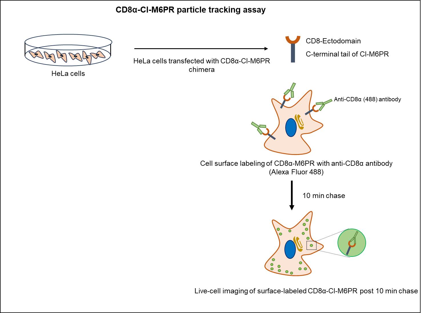
Figure 1. Schematic illustrating the CD8α-CI-M6PR trafficking assay to track motility of CD8α-CI-M6PR endosomes internalized from the cell surface.HeLa cells expressing CD8α-CI-M6PR were incubated with primary (anti-CD8α) and secondary (Alexa Fluor 488-conjugated dye) antibodies on ice to specifically label surface receptors, followed by live-cell imaging in warm media at 37 °C after 10 min of chase.
Materials and reagents
Biological materials
70%–80% confluent HeLa cells (ATCC)
Note: We have used HeLa cells for this analysis because they are easy to transfect and considerably flat for 2D analysis of endosome motility; however, other cell lines can also be used.
Reagents
Plasmid CD8α-CI-M6PR-pIRES Neo2 (a kind gift from Prof. Matthew Seaman)
GibcoTM Dulbecco’s modified Eagle medium (DMEM), high glucose, with GlutaMAXTM, sodium pyruvate (Thermo Fisher Scientific, catalog number: 10569-010), storage: 2–8 °C
Dulbecco’s phosphate buffered saline (DPBS), without calcium and magnesium (Lonza Bioscience, catalog number: 17-512F), storage: 15–30 °C
Opti-MEM® reduced serum media (Thermo Fisher Scientific, GibcoTM, catalog number: 11058021), storage: 2–8 °C
Heat-inactivated fetal bovine serum (FBS) (Thermo Fisher Scientific, Gibco TM, catalog number: 10082147), storage: -20 °C
Antibiotic-antimycotic (Thermo Fisher Scientific, GibcoTM, catalog number: 15240-062), storage: -20 °C
GibcoTM 1 M HEPES (Thermo Fisher Scientific, catalog number: 15630-080), storage: 2–8 °C
GibcoTM 100× MEM non-essential amino acid solution (Thermo Fisher Scientific, catalog number: 11140050)
GibcoTM DMEM, high glucose, HEPES, no phenol red (Thermo Fisher Scientific, catalog number: 21063029), storage: 2–8 °C
X-tremeGENETM HD transfection reagent (Roche® Life Science Products, catalog number: 6366236001)
siRNA transfection reagent Dharmafect-1 (GE Healthcare, catalog number: T-2001-03)
Mouse anti-human CD8 monoclonal antibody (BD PharmingenTM, catalog number: 555631), storage: 4 °C
Alexa Fluor 488-conjugated goat anti-mouse IgG (Thermo Fisher Scientific, catalog number: A11029), storage: 4 °C
Citrate anhydrous (HiMedia, catalog number: GRM-1023)
Sodium citrate tribasic dihydrate (Tri sodium citrate dihydrate) (Sigma, catalog number: S4641)
Citric acid buffer, pH 4.5 (see Recipes)
Recipes
Citric acid buffer, pH 4.5
Reagent Volume Citric acid anhydrous 100 mL Tri-sodium citrate dihydrate 100 mL Total 200 mL 0.1 M Citric acid anhydrous
Reagent Quantity Citric acid anhydrous 2.626 g Total 125 mL 0.1 M Tri-Sodium Citrate dihydrate
Reagent Quantity Tri-sodium citrate dihydrate 3.676 g Total 125 mL Adjust pH to 4.5 with sodium citrate.
Complete medium
Dulbecco’s modified Eagle medium (DMEM), high glucose, with GlutaMAXTM, sodium pyruvate supplemented with 10% FBS, 10 mM HEPES, 1× antibiotic-antimycotic, and 1× MEM non-essential amino acid solution
Laboratory supplies
35 mm μ-dish, high glass-bottom live-imaging dishes (ibidi, catalog number: 81158)
BD Falcon 15 mL centrifuge tubes (Corning, Falcon®, catalog number: 352096)
BD Falcon 35 mm cell culture dish (Corning, Falcon®, catalog number: 353001)
Equipment
Cell culture incubator (Eppendorf, New BrunswickTM, model: Galaxy ® 170 R)
Confocal microscope (ZEISS, model: LSM 710)
HulaMixerTM sample mixer (Thermo Fisher Scientific, catalog number: 15920D)
Software and datasets
Fiji software ( https://imagej.net/software/fiji/) 2.15.1
ZEN software, ZEN 2012 v. 8.0.1.273 (ZEISS)
Procedure
Experimental setup
Note: This protocol has been modified from CD8α-CI-M6PR trafficking assay [4], aiming to assess the motility of surface-labeled CD8α-CI-M6PR towards the Golgi in HeLa cells treated with siRNAs against a specific gene of interest.
Seed approximately 0.14 ×10⁶ HeLa cells in a 35 mm glass-bottom live-imaging dish and incubate overnight in a cell culture incubator.
Note: For transfection, seed 0.25 × 10⁶ HeLa cells and incubate overnight in a cell culture incubator.
On the following day, prepare siRNA transfection mix by combining 100 nM siRNA oligos and transfection reagent Dharmafect-1 (Dharmacon) in 200 μL of Opti-MEM and incubate the mixture at room temperature for 30 min. After incubation, add siRNA transfection mix dropwise over cells and incubate for 48 h.
After 48 h of siRNA treatment, transfect the cells with CD8α-CI-M6PR. To prepare the transfection mix, add 2 μg of CD8α-CI-M6PR-pIRES Neo2 plasmid DNA in 200 μL of Opti-MEM and X-tremeGENETM HD transfection reagent in a ratio of 1:1 (1 μg DNA: 1 μL transfection reagent). Incubate the transfection mix at room temperature for 30 min, then carefully add it dropwise over cells.
To fluorescently label the primary antibody, incubate the mouse anti-CD8 antibody along with Alexa Fluor 488-conjugated anti-mouse IgG in 1 mL of serum-free DMEM media at 4 °C for 30 min in a tube rotator.
Following 12–14 h of transfection, incubate the complex of anti-CD8α with Alexa Fluor 488-conjugated IgG with cells in a live-cell imaging dish on ice for 30 min to label the surface CD8-CI-M6PR receptors.
Note: As a control for the non-specific attachment of Alexa Fluor 488-conjugated antibodies to the plasma membrane, execute the antibody labeling and subsequent steps using untransfected cells.
After incubation, carefully aspirate the DMEM media containing anti-CD8α/Alexa Fluor 488-conjugated antibody complex.
To remove any unbound or non-specifically attached antibodies, wash the cells once with DPBS followed by two washes with ice-cold citric acid buffer, pH 4.5. Add approximately 1 mL of citric acid buffer to cells and incubate on ice for 5 min. Discard the buffer and repeat the washing step twice with citric acid buffer. Finally, add 1 mL of DPBS to remove any residual citric acid buffer from the cells.
Note: Prepare fresh citric acid buffer and use it ice-cold for washes.
After washing, add 2 mL of prewarmed phenol red–free DMEM media supplemented with 10% FBS on cells and incubate it for 10 min.
After incubation, transfer the dish to the humidified live-cell imaging chamber maintained at 37 °C with 5% CO2 and perform live-cell imaging of the transfected cells showing labeled CD8α-CI-M6PR receptors. Post 10 min chase, labeled CD8α-CI-M6PR receptors present on plasma membrane traffic to TGN due to the retrograde sorting signals present on the cytoplasmic tail of CI-M6PR.
Live-cell imaging and video acquisition
Use 512 × 512 frame size for higher acquisition speed and acquire a timelapse video of cells for approximately 200–300 frames minimum without any time interval.
Record the video of the labeled CD8α-CI-M6PR receptors for a duration not exceeding 15 min, following a 10 min chase, during which they are expected to reach TGN.
Image analysis and quantification using ImageJ/Fiji
Note: In the manuscript [6], we conducted particle tracking analysis using a semi-automated custom-written program and a MATLAB script [7]. However, in this protocol, we have presented an alternative protocol employing the TrackMate plugin for the analysis of CD8α-CI-M6PR particles.
Open the video file using Fiji. If there are multiple cells in a field, use the free-hand tool from the Fiji tool panel to select a single cell. Duplicate the selection by either using Ctrl+shift+D or go to Image menu and choose the Duplicate option. A pop-up window will appear; select the Duplicate stack option (Figure 2).
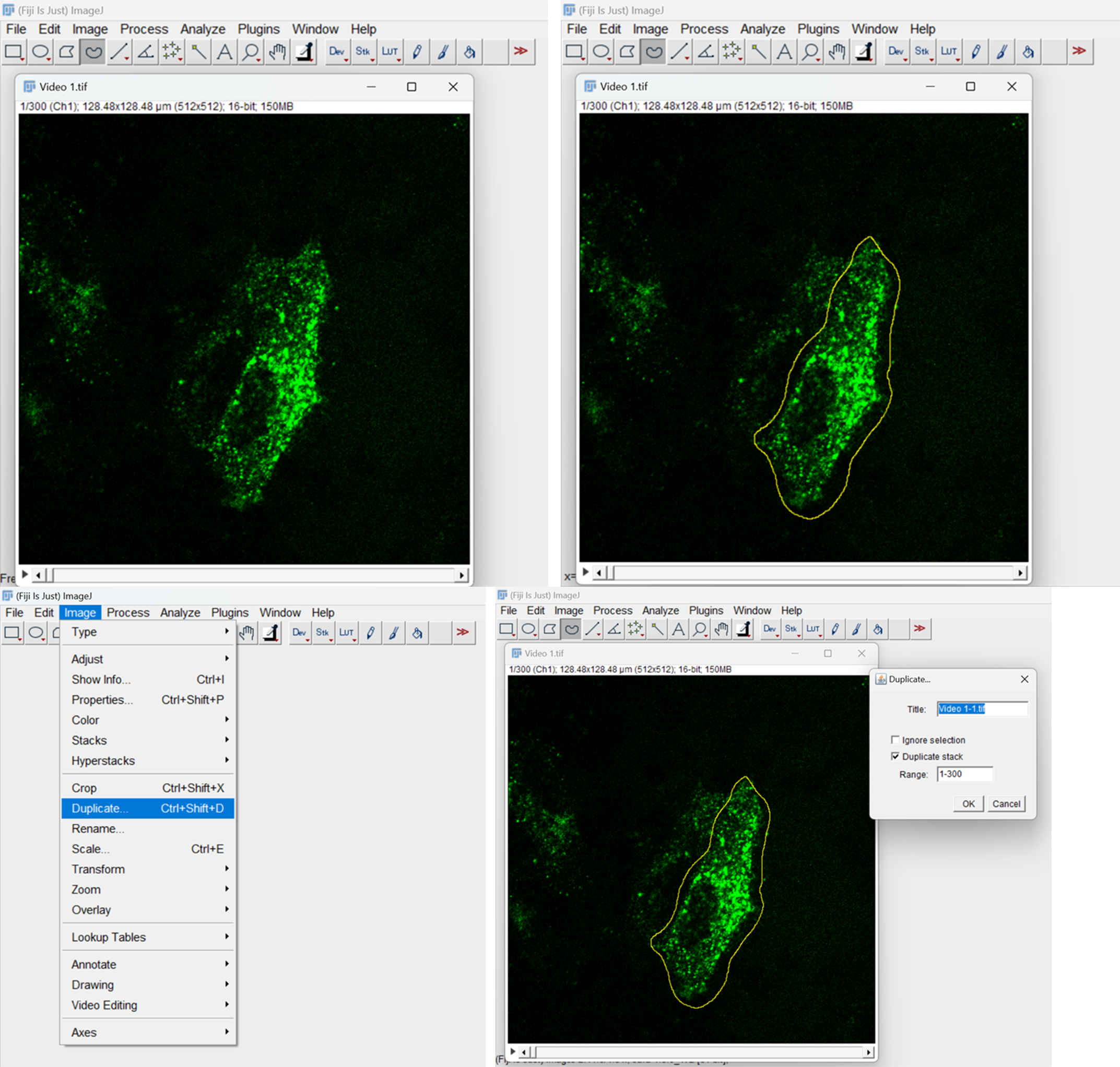
Figure 2. Duplicate video stack and select the cell for analysisRemove the background fluorescence using the Edit menu. Select the Clear outside option (Figure 3). Choose yes to the process stack option allowing it to remove the background from all frames.
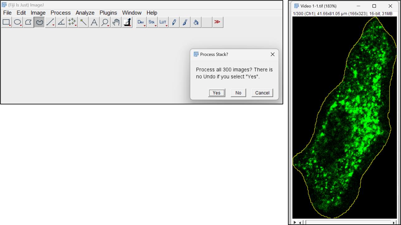
Figure 3. Clear outside from all frames of videoSubtract cytoplasmic background fluorescence from the cell to improve the endosome tracking process. Select Subtract background option in the Process menu in Fiji toolbar. Input the value of Rolling ball radius appropriately according to your background fluorescence in the video file (Figure 4).
Note: The value of Rolling ball radius should be higher than the largest object in the image.
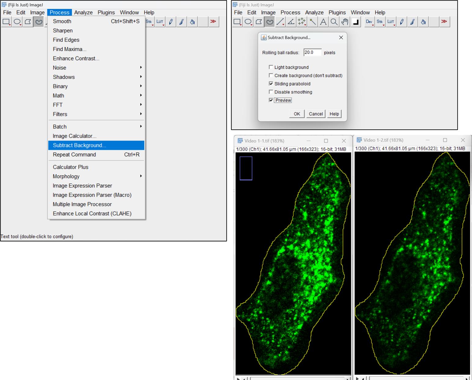
Figure 4. Background subtraction in cellPerform particle tracking on video file. Select Plugins > Tracking > TrackMate option. A dialog box will open with spatial and temporal information of the data. It provides information on pixel dimensions, number of frames, and also the dimensionality of the video file (2D or 3D lapse video). To proceed with tracking, press the Next button (Figure 5).
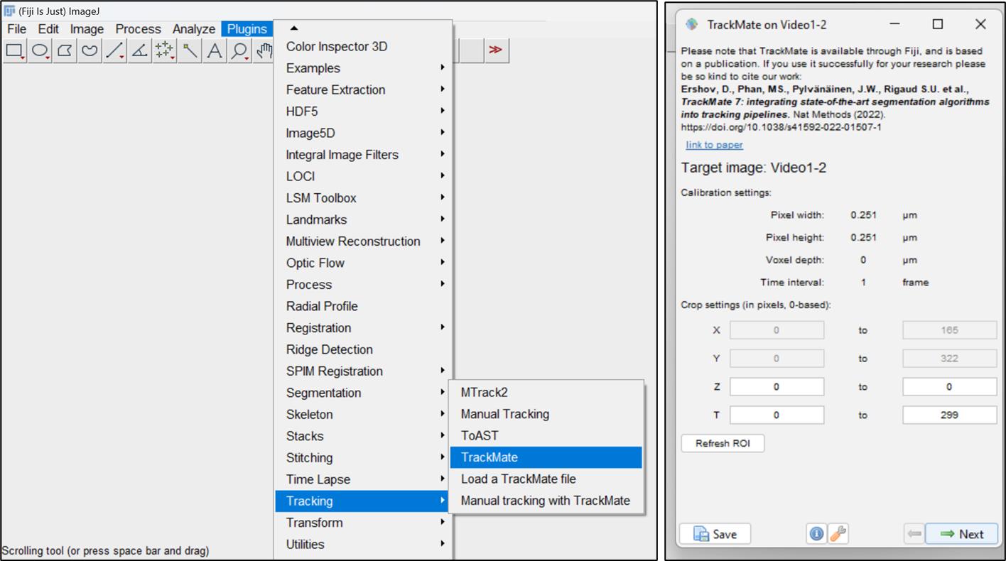
Figure 5. Particle tracking using TrackMate pluginNext, a window will open with three options as object detectors. Choose the Difference of Gaussian (DoG) detector, designed to identify round particles like endosomes and being particularly effective for particle sizes below ~5 pixels. Proceed by clicking the Next button (Figure 6).
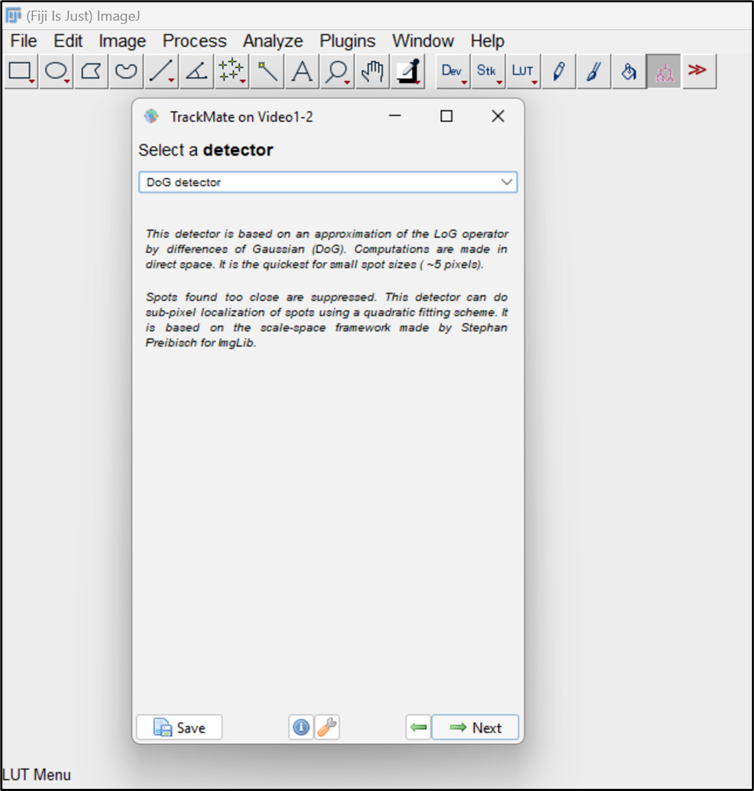
Figure 6. Selection of difference of Gaussian (DoG) detectorIn the subsequent DoG detector window, input the values for a few parameters associated with particles to be analyzed, such as Estimated Blob diameter and Quality threshold. For Estimated Blob Diameter, enter the approximate diameter of the endosomes or measure it using the line tool in Fiji. Quality threshold allows you to limit your analysis to a specific number of endosomes, excluding spots/endosomes with quality below the threshold. Click the preview button to see the selected endosomes and assess how well the parameters fit the data. Adjust the Quality threshold to eliminate any false spot intensities from the analysis. Click on Preview to see the selected spots and accordingly adjust the threshold to choose the desired endosomes. You can also see the number of endosomes that were selected for the selected threshold (highlighted here in red outline) (Figure 7). Go to the next window once adjustments have been made.
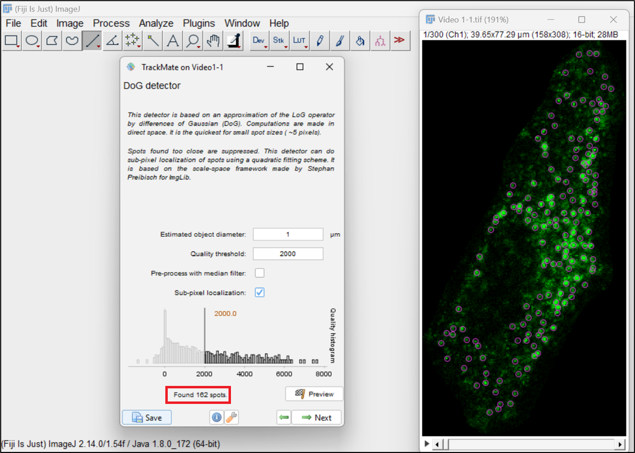
Figure 7. Difference of Gaussian (DoG) detector parameters for particlesNext, choose the HyperStack displayer, which allows you to overlay the end results over the image (Figure 8).
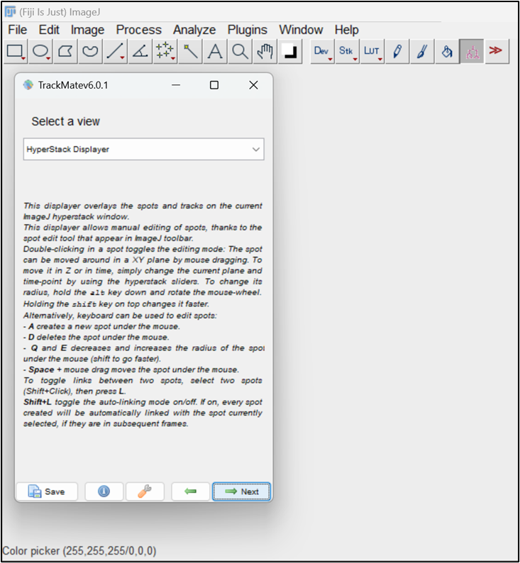
Figure 8. Choose the HyperStack displayerThis window allows you to do auto or manual thresholding to select the particles. Choose Auto here. Click Next (Figure 9).
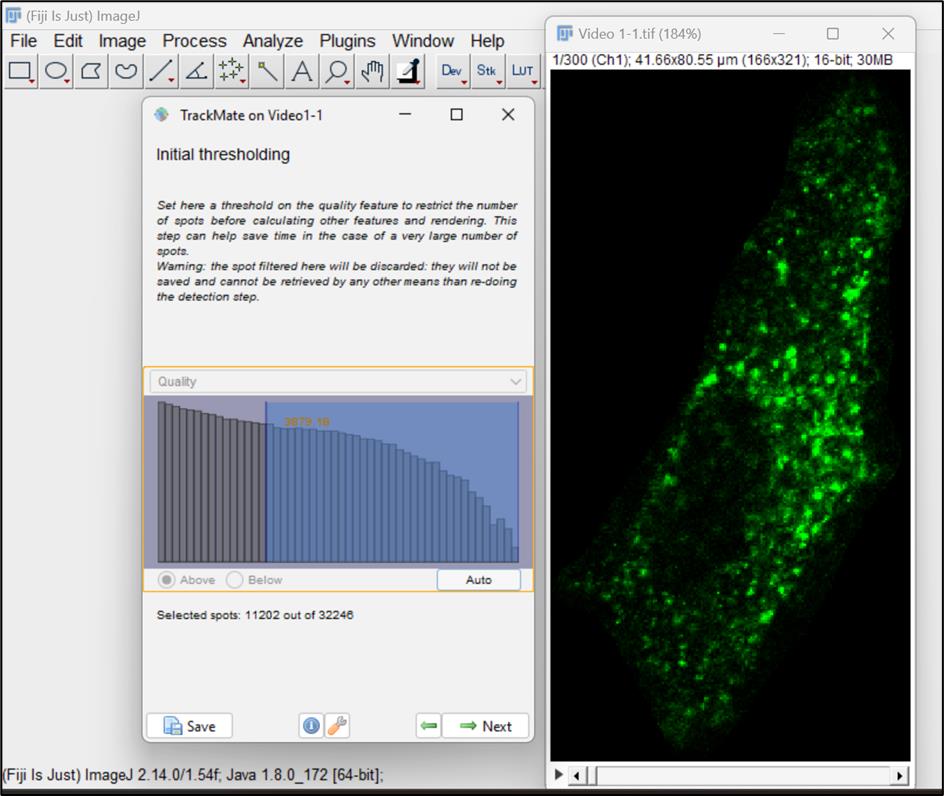
Figure 9.Thresholding on particles/spotsAt this point, we can see the spots that are selected for analysis. We can run the video and observe the spots moving through all frames. In this window, you can set filters on the spots; however, for now, we will proceed with default settings and click Next (Figure 10).
Note: You can also filter spots based on parameters like intensity, quality, radius of the particles, frame, or positions (X, Y,) and do a comparative analysis of choices.
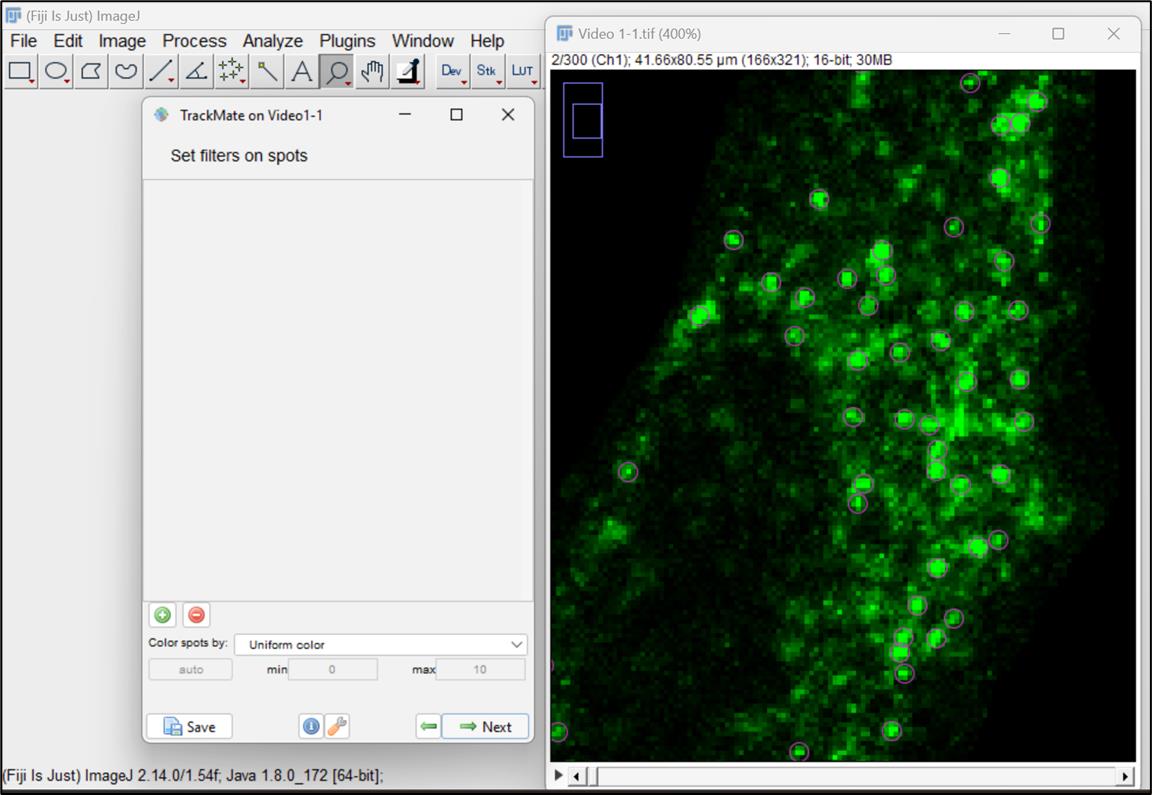
Figure 10. Set filters and choose particles or spots for analysisNow, select the simple LAP (linear assignment problem) tracker, ideal for particles undergoing Brownian motion. This tracker creates tracks by linking particles across different frames in the video (Figure 11 ).
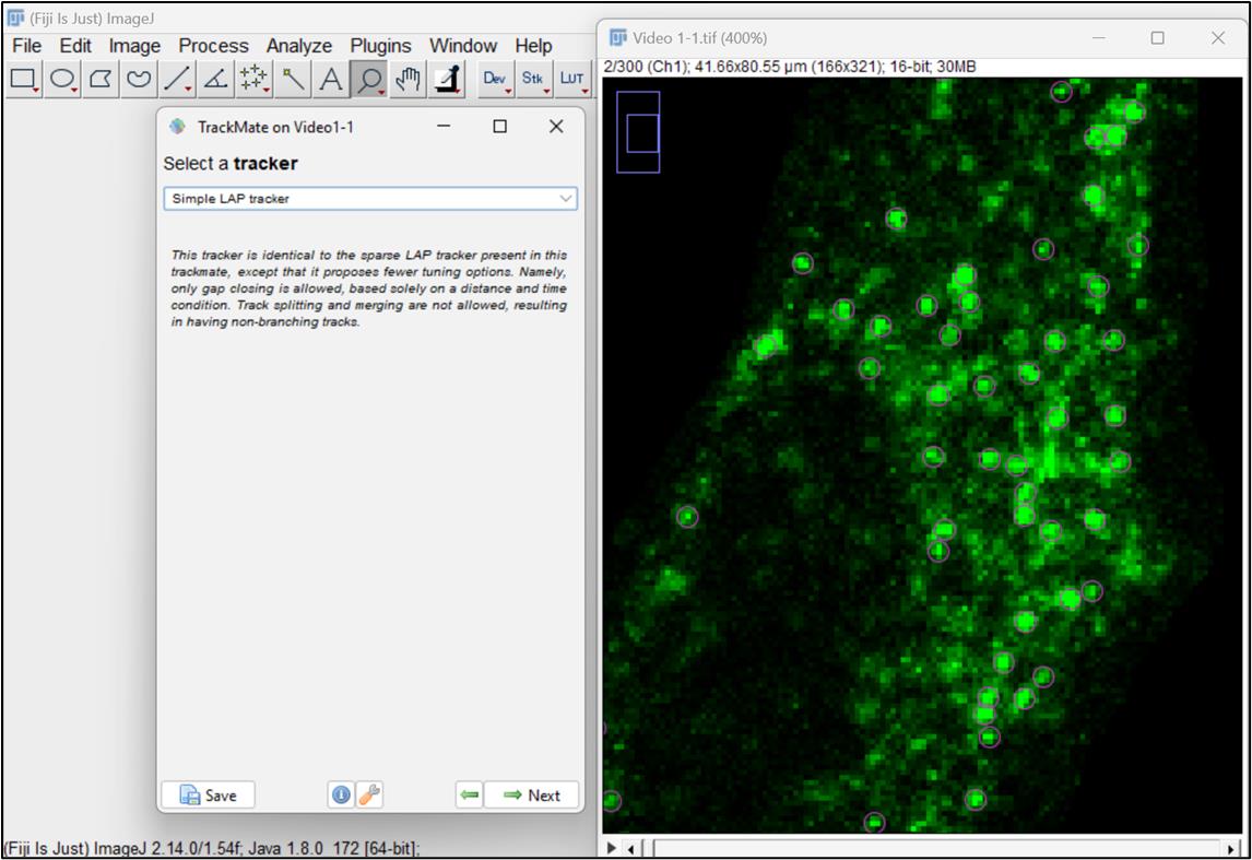
Figure 11. Selection of simple linear assignment problem (LAP) trackerNext, a LAP tracker window will open, allowing you to input parameters for particle-to-particle linking. Enter 2 μm in the option for Linking max distance, which defines the maximum distance for two spots to be linked between two frames. Put the value of Gap-closing max distance as 2 μm, meaning that it will not link any two spots that are more than two frames apart. Set Gap-closing max frame gap to 1, which is the maximum frame difference allowed for a spot to be missed for linking (Figure 12).
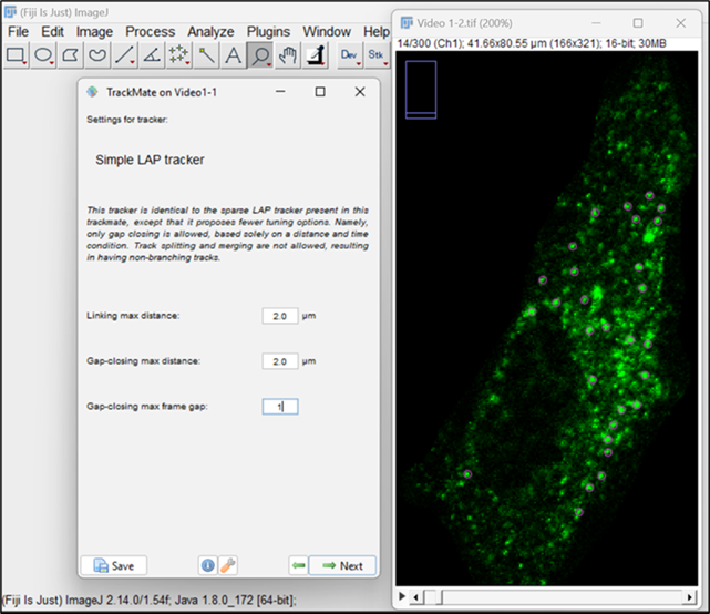
Figure 12. Configuration for linking particles by simple LAP trackerThe next window allows the visualization of the tracks generated by LAP tracker. Click Next (Figure 13).
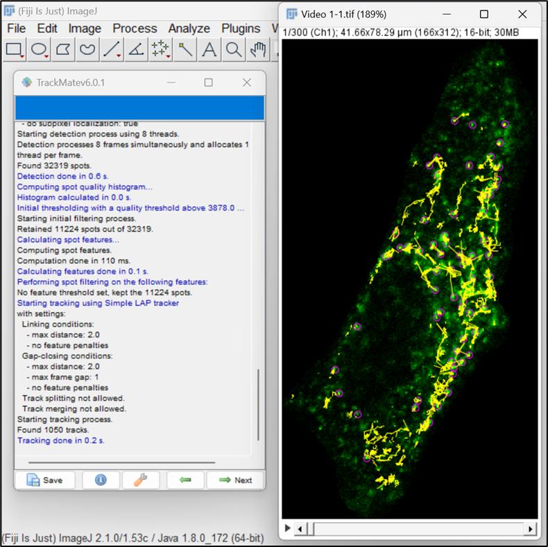
Figure 13. Tracks generated by LAP trackerThis window allows you to set filters on tracks. You can choose any option for viewing tracks, but here we have opted to set the color of the tracks based on maximal velocity. Click Next (Figure 14 ).
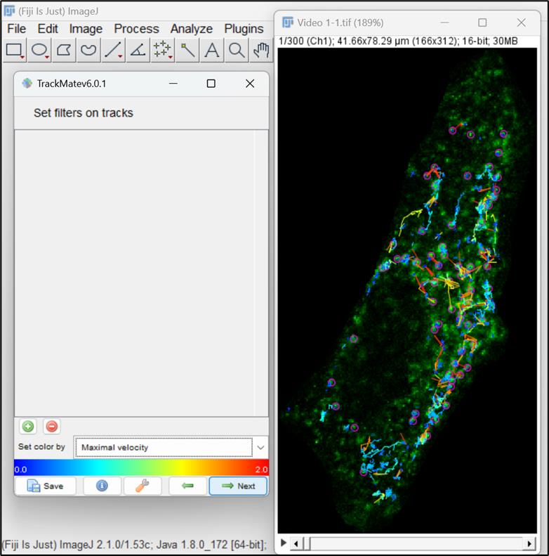
Figure 14. Color filter for visualization of tracksThe next window allows to further change the display options. Here, you can increase or decrease the size of the spot by changing its radius. Furthermore, you can also change the display of the tracks. Click on Next button. A new panel will open with options to plot different features associated with particle motility as a function of another. To continue, click on Next (Figure 15 ).
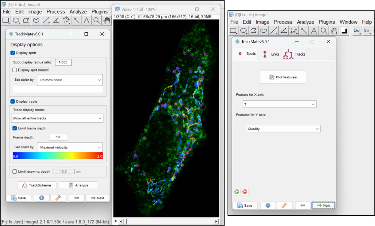
Figure 15. Display options for particles and tracksSelect Overlay option in the next window and click on Execute. A pop-up window will open, showing the total number of frames. Click on ok. You can save the video with all the captured tracks (Figure 16).
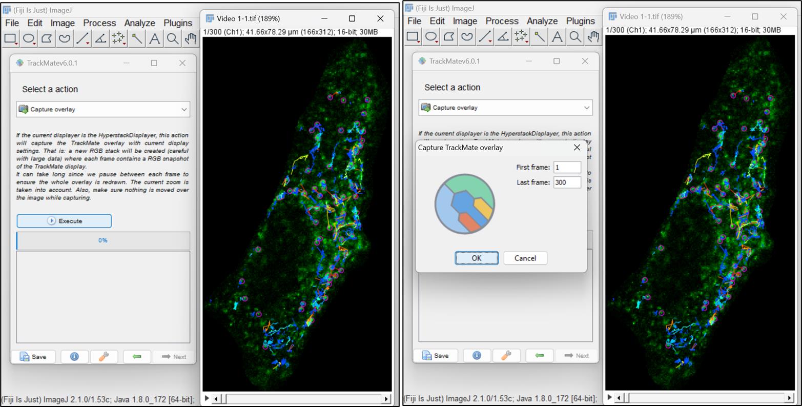
Figure 16. TrackMate features and analysisTo obtain measurements associated with particle/spot’s motion such as distance, displacement, maximum speed, and duration of a track, go back to the Display options window (shown in Figure 15) and click on Analysis. Three different windows will open, providing information on quantitative parameters for all the tracks associated with the particle motion (Figure 17).
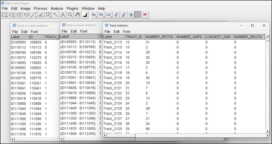
Figure 17. Track analysis tables showing different kinetic parameters associated with particle motion
Data analysis
From the data extracted from the track statistics file or table, we can acquire values such as track duration, displacement, mean velocity, and maximum speed for all the tracks identified by the LAP tracker. In the video, we have detected roughly ~1,000 tracks by linking two spots over time. Each track encompasses values for displacement, duration, and velocity. Displacement signifies the distance between spots in consecutive frames, while duration indicates the time span. Velocity values denote the link velocity defined for each link between two spots. Subsequently, we can compute and plot the median, maximum, minimum, and average velocities from link velocities under different conditions or treatments. Analyze the tracks from approximately 7–10 cells and plot the values for each quantitative parameter against various treatments. Further, calculate the statistical significance of differences in mean values between two or more conditions by utilizing either an unpaired two-tailed Student’s t-test or analysis of variance (ANOVA), respectively. These tests are applicable when the data approximately follows a normal distribution and satisfies assumptions such as homogeneity of variances. For non-normal distributions, which lack symmetry, statistical comparisons are done between the medians of the two groups using Mann-Whitney U test.
Validation of protocol
This protocol has been used and published in the following research article:
Rawat, S. et al. (2022). RUFY1 binds Arl8b and mediates endosome-to-TGN CI-M6PR retrieval for cargo sorting to lysosomes. J. Cell Biol. (Figure 10, panel D)
Note: This article has used a semi-automated custom-written program and a MATLAB script [7], but here we have employed an alternative approach using TrackMate plugin for the particle analysis.
Acknowledgments
The authors adapted and modified this protocol from a previously published study [4] and validated it in a recently described study [6]. The authors would like to thank Prof. Matthew Seaman (University of Cambridge, UK) for sharing the CD8α-CI-M6PR construct. S. Rawat acknowledges fellowship support from University Grants Commission. M. Sharma would like to acknowledge funding support from the Department of Biotechnology (DBT)/Wellcome Trust India Alliance Senior Fellowship (IA/S/19/1/504270), SERB-POWER Grant (SPG/2021/002790), and Janaki Ammal-National Women Bioscientist Award (BT/HRD/NWBA/39/01/2018-19). M. Sharma also acknowledges the infrastructure and financial support from IISER Mohali.
Competing interests
The authors declare no competing financial interests.
References
- Calcagni, A., Staiano, L., Zampelli, N., Minopoli, N., Herz, N. J., Di Tullio, G., Huynh, T., Monfregola, J., Esposito, A., Cirillo, C. et al. (2023). Loss of the batten disease protein CLN3 leads to mis-trafficking of M6PR and defective autophagic-lysosomal reformation. Nat. Commun. 14(1): 3911. https://doi.org/10.1038/s41467-023-39643-7
- Cui, Y., Yang, Z., Flores-Rodriguez, N., Follett, J., Ariotti, N., Wall, A. A., Parton, R. G. and Teasdale, R. D. (2021). Formation of retromer transport carriers is disrupted by the Parkinson disease-linked Vps35 D620N variant. Traffic 22(4): 123–136. https://doi.org/10.1111/tra.12779
- Hirst, J., Futter, C. E. and Hopkins, C. R. (1998). The kinetics of mannose 6-phosphate receptor trafficking in the endocytic pathway in HEp-2 cells: the receptor enters and rapidly leaves multivesicular endosomes without accumulating in a prelysosomal compartment. Mol. Biol. Cell 9(4): 809–816. https://doi.org/10.1091/mbc.9.4.809
- Seaman, M. N. (2004). Cargo-selective endosomal sorting for retrieval to the Golgi requires retromer. J. Cell Biol. 165(1): 111–122. https://doi.org/10.1083/jcb.200312034
- McKenzie, J. E., Raisley, B., Zhou, X., Naslavsky, N., Taguchi, T., Caplan, S. and Sheff, D. (2012). Retromer guides STxB and CD8-M6PR from early to recycling endosomes, EHD1 guides STxB from recycling endosome to Golgi. Traffic 13(8): 1140–1159. https://doi.org/10.1111/j.1600-0854.2012.01374.x
- Rawat, S., Chatterjee, D., Marwaha, R., Charak, G., Kumar, G., Shaw, S., Khatter, D., Sharma, S., de Heus, C., Liv, N., et al. (2023). RUFY1 binds Arl8b and mediates endosome-to-TGN CI-M6PR retrieval for cargo sorting to lysosomes. J. Cell Biol. 222(1). https://doi.org/10.1083/jcb.202108001
- Mohan, N., Sorokina, E. M., Verdeny, I. V., Alvarez, A. S. and Lakadamyali, M. (2019). Detyrosinated microtubules spatially constrain lysosomes facilitating lysosome-autophagosome fusion. J. Cell Biol. 218(2): 632–643. https://doi.org/10.1083/jcb.201807124
Article Information
Copyright
© 2024 The Author(s); This is an open access article under the CC BY-NC license (https://creativecommons.org/licenses/by-nc/4.0/).
How to cite
Readers should cite both the Bio-protocol article and the original research article where this protocol was used:
- Rawat, S. and Sharma, M. (2024). CD8α-CI-M6PR Particle Motility Assay to Study the Retrograde Motion of CI-M6PR Receptors in Cultured Living Cells. Bio-protocol 14(9): e4979. DOI: 10.21769/BioProtoc.4979.
- Rawat, S., Chatterjee, D., Marwaha, R., Charak, G., Kumar, G., Shaw, S., Khatter, D., Sharma, S., de Heus, C., Liv, N., et al. (2023). RUFY1 binds Arl8b and mediates endosome-to-TGN CI-M6PR retrieval for cargo sorting to lysosomes. J. Cell Biol. 222(1). https://doi.org/10.1083/jcb.202108001
Category
Cell Biology > Cell imaging > Live-cell imaging
Cell Biology > Cell-based analysis > Transport
Do you have any questions about this protocol?
Post your question to gather feedback from the community. We will also invite the authors of this article to respond.