- Protocols

- Articles and Issues
- For Authors
- About
- Become a Reviewer

Automated Layer Analysis (ALAn): An Image Analysis Tool for the Unbiased Characterization of Mammalian Epithelial Architecture in Culture
Published: Vol 14, Iss 8, Apr 20, 2024 DOI: 10.21769/BioProtoc.4971 Views: 4207
Reviewed by: Ralph Thomas BoettcherKaty RothenbergSusanne ReinhardtHsih-Yin Tan
Original research article
The authors used this protocol in:

Mar 2023
Advertisement


Protocol Collections
Comprehensive collections of detailed, peer-reviewed protocols focusing on specific topics


Related protocols
Abstract
Cultured mammalian cells are a common model system for the study of epithelial biology and mechanics. Epithelia are often considered as pseudo–two dimensional and thus imaged and analyzed with respect to the apical tissue surface. We found that the three-dimensional architecture of epithelial monolayers can vary widely even within small culture wells, and that layers that appear organized in the plane of the tissue can show gross disorganization in the apical-basal plane. Epithelial cell shapes should be analyzed in 3D to understand the architecture and maturity of the cultured tissue to accurately compare between experiments. Here, we present a detailed protocol for the use of our image analysis pipeline, Automated Layer Analysis (ALAn), developed to quantitatively characterize the architecture of cultured epithelial layers. ALAn is based on a set of rules that are applied to the spatial distributions of DNA and actin signals in the apical-basal (depth) dimension of cultured layers obtained from imaging cultured cell layers using a confocal microscope. ALAn facilitates reproducibility across experiments, investigations, and labs, providing users with quantitative, unbiased characterization of epithelial architecture and maturity.
Key features
• This protocol was developed to spatially analyze epithelial monolayers in an automated and unbiased fashion.
• ALAn requires two inputs: the spatial distributions of nuclei and actin in cultured cells obtained using confocal fluorescence microscopy.
• ALAn code is written in Python3 using the Jupyter Notebook interactive format.
• Optimized for use in Marbin-Darby Canine Kidney (MDCK) cells and successfully applied to characterize human MCF-7 mammary gland–derived and Caco-2 colon carcinoma cells.
• This protocol utilizes Imaris software to segment nuclei but may be adapted for an alternative method. ALAn requires the centroid coordinates and volume of nuclei.
Graphical overview

Background
We developed a tool for the unbiased analysis of layer architecture (Automated Layer Analysis or ALAn) for two reasons. Firstly, cultured epithelial architecture can vary drastically between experiments, and we found this can be the case even across a single 1 mm2 culture well [1]. Secondly, epithelial tissues are commonly considered to be pseudo–two dimensional, meaning that architecture is primarily considered with respect to the tissue plane/surface. We found that this perspective is not always predictive of architecture with respect to tissue depth (the apical-basal axis) [1]. We are interested in the mechanical and biological parameters that contribute to epithelial layer architecture and we developed this tool to quantify architecture development over time and test the effect of plating density, culture time, and presence of cadherin-mediated adhesion on architecture. Due to the variability in the shape of layers and the complexity of attempting to perform 3D analysis manually, it was important to us to develop an unbiased and automated tool that requires as little user input as possible. As a consequence of developing ALAn, we identified a developmental series of layer architectures that progress through the process of epithelialization, whereby individual cells form a tissue layer [1,2]. Our quantifications of cell height, cell density, and circularity show distinct morphological regimes for each architecture.
Several tools exist for the analysis of epithelial topology in the plane of the tissue [3–6]. As far as we are aware, ALAn is the first to characterize and quantify the apical-basal topology of cultured layers. To do so, the tool makes use of two pieces of spatial information: 1) a projection of actin signal intensity and 2) the positions of cell nuclei in the apical-basal dimension. Using this information, ALAn outputs layer density and layer height and assigns each layer to one of four organized categories representing a developmental series (Immature, Intermediate A, Intermediate B, and Mature) or a fifth category of exclusion (Disorganized) [1,2]. ALAn also utilizes existing Python libraries to output in-plane quantifications of cell shape.
Confluent epithelial tissues in culture transition between distinct developmental architectures as they proliferate and therefore densify [1,2]. ALAn makes architectural classifications based on plots of the average spatial distributions of nuclei and actin across the apical-basal depth of a 3D-imaged region. At sparse densities, cultured epithelial cell layers have a squamous morphology and are characterized by a lack of defined lateral surfaces; these are classified as Immature. The spatial plots of Immature layers have the peak of nuclear distribution located at, or occasionally above, the peak actin intensity (Figure 1A). At intermediate densities, layers develop lateral cell–cell borders and rounded cell apices; these are classified as Intermediate. The Intermediate category is split into two. The first of these, called Intermediate A (IntA), are layers where cells exhibit an asymmetric actin intensity profile with a single peak closer to the apical surface than the nuclear profile (Figure 1B). If the plot of actin exhibits a shoulder (corresponding to distinct lateral and apical pools of actin), then layers are classified as Intermediate B (IntB) or Mature (Figure 1C–1D) [2]. ALAn uses the derivative of the actin intensity plot to detect this shoulder. If the derivative is two-peaked, the ratio of the right peak to the left peak is used. A ratio of less than 1 defines IntB layers, and a ratio of greater than 1 is classified as a Mature layer. The Disorganized architectural category of epithelial cell culture is characterized by a failure to achieve a regular monolayered architecture in the apical-basal axis and therefore is characterized by broad nuclear and actin profiles (Figure 1E). Disorganization occurs when the underlying cell culture substrate area is insufficient to accommodate the number of cells seeded onto the plate [1].
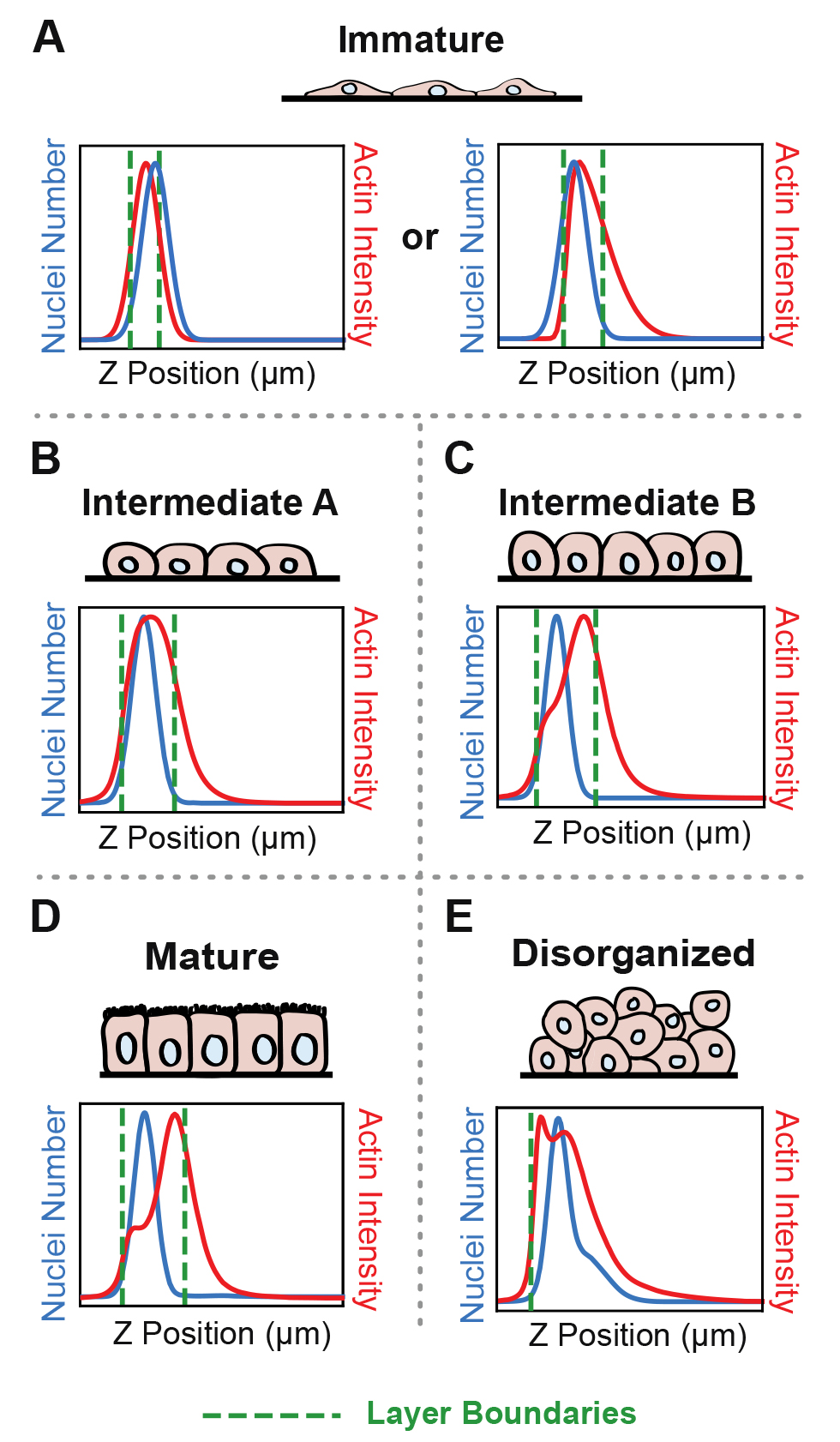
Figure 1. Epithelial architecture categories and the distinctive spatial distribution profiles of nuclei and actin positions in the apical-basal (z) axis that Automated Layer Analysis (ALAn) uses to categorize them
Materials and reagents
Reagents
Dulbecco’s phosphate buffered saline (dPBS) (Sigma-Aldrich, catalog number: SKU D1408
Phosphate buffered saline (PBS) (such as tablets from Thermo Fisher, Invitrogen, catalog number: 003002)
Paraformaldehyde, 37% (Fisher Scientific, catalog number: F79-500)
Tween 20 detergent (Sigma, catalog number: SKU 11332465001)
Vectashield antifade mounting medium with DAPI (Vector Laboratories, catalog number: SKU H-1200)
Fluorescein phalloidin (Thermo Fisher, Invitrogen, catalog number: F432)
Collagen IV coated 8-well µ-slide, #1.5 polymer coverslip, sterilized (Ibidi, catalog number: 80822)
Equipment
Spinning disc confocal unit coupled to a Nikon Ti-E inverted microscope and Zyla 4.2 sCMOS camera; 405 nm and 488 nm laser lines; 40× NA 1.15 water immersion lens (Andor, Oxford Instruments model: Dragonfly 200)
Computer workstation with a minimum 8 GB RAM, AMD, or NVIDIA 2 GB Graphics card and monitor with 1,280 × 1,024 pixels.
Software and datasets
Fusion (Version 2.3, Andor). Optional; used for image acquisition
Imaris (Versions 9.7, 9.8, 9.9, or 10.0, Oxford Instruments). Optional, used for nuclei segmentation
FIJI, ImageJ2 distribution (Version 2.14.0) [7,8]
Microsoft Excel (Version independent)
Anaconda distribution (Version 3, 2023.07-2)
Code can be obtained from GitHub: https://github.com/Bergstralh-Lab/ALAn (Access date, 03/13/2024)
Collation_Imaris2ALAn.ipynb
ALAn_v3.ipynb
Procedure
Cell culture and imaging (suggested approach)
Cell culture, fixation, and staining
Culture mammalian cells in Ibidi wells.
After the desired period of culture time, remove the culture media and wash cells once with 250 μL of dPBS.
Add 200 μL of a solution of 3.7% paraformaldehyde diluted in PBS with 2% Tween 20 to the well and incubate for 10 min at room temperature.
Wash the cells three times with 250 μL of PBS with 0.2% Tween 20, letting the wash solution sit in each well for 10 min between washing steps.
Dilute fluorescein phalloidin 1:500 in PBS with 0.2% Tween 20 and add 250 μL to each well. Incubate for 12–24 h at 4 °C.
Remove phalloidin solution and rinse with PBS with 0.2% Tween 20 three times.
Add approximately 500 μL (or at least enough to fully cover the cell layer) of Vectashield with DAPI to the well.
Confocal imaging
Cells can be imaged directly in the Ibidi wells through the #1.5 polymer coverslip bottom using an inverted confocal microscope. Image a region in XY with an area of at least 60 μm × 60 μm at Nyquist resolution at a minimum of 512 × 512 pixels.
Image actin stained by FITC-conjugated phalloidin using the 488 nm line and DNA stained by DAPI using the 405 nm line. Use standard imaging techniques to set acquisition parameters to ensure that you are taking advantage of the full dynamic imaging range and not saturating pixels.
Note: Any saturation will invalidate the use of ALAn.
Take confocal z-stacks at a spacing of no greater than 0.5 μm, preferably Nyquist sampling (select Auto step size in the Z-scan settings in Fusion), starting from beneath the bottom of the chamber slide where no actin (FITC) signal can be detected and ending above the layer where no more actin signal can be detected.
Preparation of data for input into ALAn
Segmentation of nuclei using Imaris
Save files using the following name format: “Identfier1_Identifier2_Identifier3_Identifier4.ims” where the identifiers are the experimental parameters that you would like to log (for example, “MDCKcells_GeneKnockOut1_PlatingDensity100k_48hrsGrowth.ims”).
Load the files to be analyzed into the Imaris arena using the Observe Path function.
Select the image to be analyzed and open in the Surpass view.
Go to the 3D View menu and select Cells .
Select the Add new Cells function to begin segmentation.
Use the default settings to segment nuclei and cell borders (although we will skip the cell borders segmentation) and deselect Segment only a Region of Interest.
Use the blue arrow to move to nuclei detection. Do not use the green arrow.
Set your source channel to the DNA-stained channel (DAPI-stained 405 channel using the above protocol).
Set the expected nucleus diameter based on the cell types. (For MDCK cells, we suggest a value of 7.3 μm.)
Ensure that the smooth feature is auto selected and set to a width of 1/10th of the nucleus diameter.
Select Split Nuclei by Seed Points.
Use the blue arrow to move to Filter Nuclei Seed Points.
Set the minimum Quality factor to 4.
Note: This value is set to be relatively low because, at this stage of the segmentation process, it is best to find as many nuclei as possible. It is easy to remove nuclei in ALAn, but impossible to add more.
Use the blue arrow to move to Nuclei Threshold.
Set the “Nuclei Threshold (absolute intensity)” to a value that accurately segments the nuclei in the interactive view (Figure 2A). (Check to ensure that this value does not include the peak on the histogram that corresponds to the background signal peak. If it does, then adjust the threshold up until it is past the peak.)
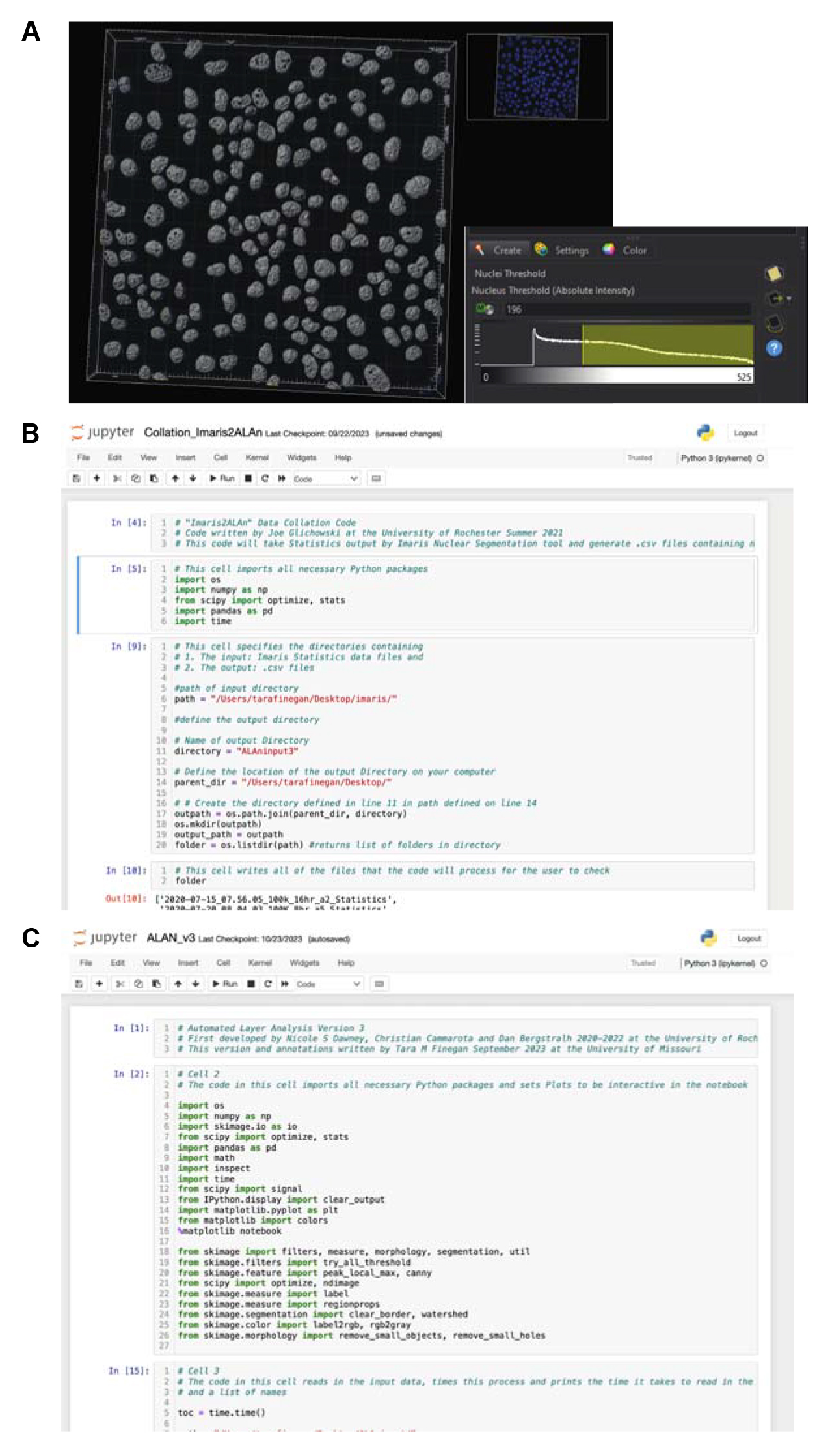
Figure 2. Screenshots showing key steps from the protocol. A. Screenshot from Imaris showing the nuclear segmentation step. Users must choose a nucleus threshold value such that nuclei are accurately segmented and segmented seeds are not touching where possible. B and C. Screenshots of Jupyter Notebook showing open Collation_Imaris2AlAn (B) and ALAn_v3 code (C).Use the blue arrow to move to Filter Nuclei.
When the Thresholding ends, click the orange X. Do not do any further filtering at this point unless you disagree with the segmentation.
Save the segmented summary statistics by first selecting the Statistics option and then selecting the Export All Statistics to File option. It is helpful to save all Imaris segmentation files in one directory, separate from the original .ims image files. The Imaris output creates a folder of files that contain the positional and volumetric information of segmented nuclei.
Download Collation_Imaris2ALAn.ipynb from the Bergstralh lab GitHub. This data will convert the Imaris statistics into .csv data files that can be read into ALAn.
Open Jupyter Notebook from Anaconda navigator. This will open Jupyter Notebook in a new browser window of your default browser. A navigation menu of the files on your computer is shown.
Navigate to the location of the “Collation_Imaris2ALAn.ipynb” file on your computer and open this Notebook (Figure 2B).
Run the code in Jupyter Notebook cell 2, which imports the necessary Python packages.
Define the input directory path, where the Imaris Statistics files are located, on Jupyter Notebook cell 3, line 6.
Define the output directory name on Jupyter Notebook cell 3, line 11, and the directory location of this directory on Jupyter Notebook cell 3, line 14. This will be the location where .csv files containing the necessary nuclei positions will be saved.
Run through all code in the “Collation_Imaris2ALAn” file.
Required data if you segment nuclei using a method not using Imaris as described in Section 1
Segment nuclear positions and extract information about the volume and centroid of nuclei in the image file.
Generate a .csv file with four columns. Column 1: X coordinate of nucleus center; Column 2: Y coordinate of nucleus center; Column 3: Z coordinate of nucleus center; Column 4: Volume of Nucleus. Rows correspond to each segmented nucleus.
Add heading titles to row 1. A1 = Nucleus Position X; B1 = Nucleus Position Y; C1 = Nucleus Position Z; D1 = Nucleus Volume.
Scale XY confocal slices to 512 × 512 pixels.
This can be done in Imaris in the Edit menu by selecting Resample 3D and resizing the X and Y values as 512. Make sure to select Fixed Ratio X/Y, not Fixed Ratio X/Y/Z.
Determine the spatial bounds of the image.
Open the original image file using FIJI.
Select Show Info from the Image menu.
Identify the X, Y, and Z spatial bounds of the image file in the Show Info panel values ExtMax0 through ExtMin2. ExtMax0 =X max; ExtMax1 = Y max; ExtMax2 = Z max; ExtMin0 = X min; ExtMin1 = Y min; ExtMin2 = Z min.
Open the .csv file containing the segmented nuclei positions using Microsoft Excel.
Name column E “Positions.”
Paste values ExtMax0 through ExtMin2 into Excel notebook cells E2–E7.
Save confocal stacks as .tiff files in the same folder as the corresponding .csv files containing the nuclei segmentation information. This can be done by opening proprietary file images in FIJI and Selecting Save as > Tiff in the File menu.
Ensure that the corresponding .csv files containing the nuclear and layer positional information and the .tiff files containing the confocal stack images have the same name. ALAn will read both files and perform an analysis of these partner files.
Use ALAn to batch process and analyze data
Download “ALAn_v3.ipynb” from the Bergstralh lab GitHub. This is the main data analysis code.
Open Jupyter Notebook from Anaconda navigator. This will open Jupyter Notebook in a new browser window of your default browser. A navigation menu of the files on your computer is shown.
Navigate to the location of the “ALAn_v3.ipynb” file on your computer and open this Notebook (Figure 2C).
Run the code in Jupyter Notebook cell 2, which imports the necessary Python packages.
Change the code on Jupyter Notebook cell 3, line 7 to the path where your input partner .csv and .tiff files are located.
Run the code in Jupyter Notebook cell 3. The data will be imported into two lists. All of the information in the .csv files will be converted into a list of pandas DataFrames (list_of_dfs), and all .tiffs will be read in as a list of 4D numpy arrays (list_of_unshuffled_images). Any .tiff or .csv file that does not have a partner file with the same name will not be added to these lists. A third list (list_of_names) will be generated to keep track of which image name is stored in each of the elements.
Check that the file names, number of input images, and dimensions of the three lists are the same, as shown in the output text below the Jupyter Notebook cell.
Run the code in Jupyter Notebook cell 4. This will load all of the functions of ALAn. Note: A description of each function and a description of its inputs and outputs are in the README.md file on the Bergstralh-Lab/ALAn GitHub page.
Change the input parameters of the batch_process function on code line Jupyter Notebook cell 5, line 2.
First, define the channel that represents the image actin signal in the .tiff file (this can be determined by opening the .tiff in FIJI) (0 = first channel, 1 = second channel, etc.).
Second, change the name that you would like to save your output .csv file as.
Run the code in Jupyter Notebook cell 5. This will process all of the input images as a batch. A timer will output the time taken to run this function.
Open the output .csv file, which has the name as defined on Jupyter Notebook cell 5, line 4 as the last parameter of the batch_process function. The directory will be the same as your input files. Check that a valid output has been generated. The basic outputs of ALAn are:
Column A: Element number used by ALAn for each input.
Column B: Root name of input .tiff and .csv files.
Column C: Layer determination; ALAn makes a categorization of the layer into the following categories: Disorganized, Immature, Intermediate A, Intermediate B, and Mature. For a full explanation of these categories see Dawney et al. [1] and Cammarota et al. [2].
Column D: Number of cells identified in the basal tissue layer.
Column E: Number of cells identified above the basal tissue layer.
Column F: Total number of cells (sum of columns D and E).
Column G: Cell density of identified tissue layer per unit culture area.
Column H: Height of identified tissue layer.
Column I: Percentage of total cells above the layer.
Column J: Average area of cells in the plane of the tissue.
Column K: Average cell perimeter in the plane of the tissue.
Column L: Average cell circularity in the plane of the tissue.
Use of ALAn to make diagnostic/informative plots and visuals
For any dataset, the functions of ALAn can be used to generate diagnostic and data outputs and figures. Here, we provide a protocol for running the functions that provide the most informative figure outputs for the analysis of the data. An optional input of save_name = “string” allows you to save this plot as a .pdf. Figures should be generated in an embedded figure in the Jupyter Notebook (defined by code on Jupyter Notebook cell 2, line 16: “%matplotlib notebook”).
Determine the element number for the dataset of interest from the output .csv file of the batch_process function.
In a new Jupyter Notebook cell, define your dataset of interest by typing “I = n’ where n is the element number of your chosen dataset.
In any subsequent Jupyter Notebook cell, you can run the clear_debris function by typing “clear_debris(list_of_dfs[i], plot = True)” and run the Jupyter Notebook cell. This function provides data on which objects identified by the nuclear segmentation input are considered as real cells and used for analysis. A histogram showing the distribution of nuclear volumes in μm3 (X-axis) against the frequency of these volumes is output (Figure 3A). The objects discarded as debris are shown in blue, and the nuclei identified as valid are orange. A pandas DataFrame containing the nuclei identified as true datapoints is output (df_cleared) and printed below the figure.
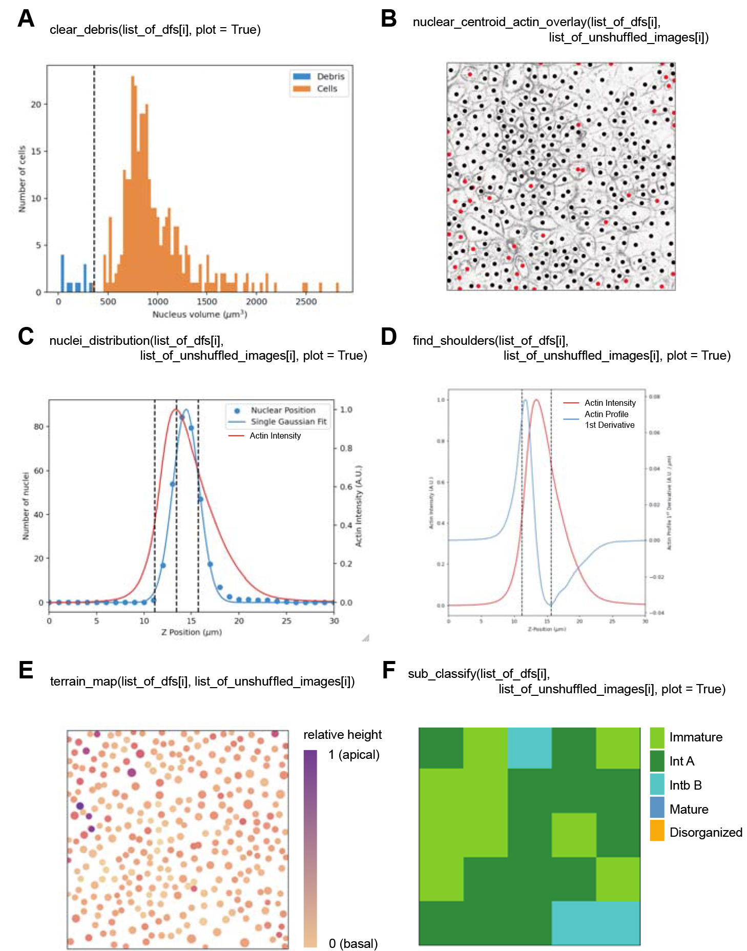
Figure 3. Diagnostic and informative plots generated by Automated Layer Analysis (ALAn). A. The clear_debris function outputs a histogram showing the frequency of segmented objects with respect to their volume that was input into ALAn. The orange bars represent nuclei identified as real and the blue bars represent debris that is removed from the analysis. A dotted line indicates the threshold volume above which a nucleus is considered real. B. The nuclear_centroid_actin_overlay function outputs an image that displays the centroid position of the segmented nuclei overlaid onto the .tiff image of the actin signal projected on the XY plane of the tissue. C. The nuclei_distribution function outputs a plot showing both the projected signal of actin (red) and the nuclear distribution (blue), fit with a Gaussian, with respect to the depth of the tissue. The tissue layer top, bottom, and peak position of the actin signal are shown by dotted lines. D. The find_shoulders function outputs a plot of the actin signal (red) and the first derivative of this plot (blue) with respect to the tissue depth. The tissue layer top, bottom, and peak position of the actin signal are shown by dotted lines. E. The terrain_map function outputs a map of the position of the centroids of nuclei projected onto the XY plane of the tissue, displayed as dots. The size of the dots shows relative volumes of nuclei. The color of the dots represents the relative positions of the nuclei with respect to the depth of the tissue. The color scale goes from light orange (most basal) to purple (most apical). F. The sub_classify function outputs a map representing the XY field of view of the input 512 × 512 pixel .tiffs broken into 100 × 100 pixel sections, color-coded by the layer category as determined by the original version of ALAn. “lawngreen” = Immature, “forestgreen” = Intermediate A, “darkturquoise” = Intermediate B, “steelblue” = Mature, “orange” = Disorganized.In any subsequent Jupyter Notebook cell, you can run the nuclear_centroid_actin_overlay function by typing “nuclear_centroid_actin_overlay(list_of_dfs[i], list_of_unshuffled_images[i]).” Use this function to test the input nuclear segmentation and clear_debris functions to ensure that the nuclei used by ALAn are reasonable. A figure is generated in the Notebook showing the nuclear centroid positions in the tissue plane are overlayed with the actin channel to view the position of nuclei within each cell (Figure 3B). Black dots indicate real nuclei and red dots indicate false nuclei as defined by clear_debris.
If you are not happy with the cutoff volume of real nuclei, you can change the value that is used to define what a real nucleus is in the clear_debris function. This is currently set to 1.5 standard deviations below the average nuclear volume (defined on Jupyter Notebook cell 4, line 97).
In any subsequent Jupyter Notebook cell, you can run the nuclei_distribution function by typing “nuclei_distribution(list_of_dfs[i], list_of_unshuffled_images[i], plot = True).” This function determines if the layer is organized into a monolayer or not and returns a classification as Organized or Disorganized. A plot showing the projected number of nuclei and actin intensity (double Y-axis) across the depth of the layer, Z position in µm (X-axis) is generated in the Notebook (Figure 3C). This is a useful figure to interrogate the organization of cells across the depth of the tissue.
In any subsequent Jupyter Notebook cell, you can run the find_shoulders function (Figure 1D) by typing “find_shoulders(list_of_dfs[i], list_of_unshuffled_images[i], plot = True).” This function determines whether the plot of actin intensity across the depth of the tissue has a shoulder. The output is a plot of actin intensity and the first derivative of the actin profile (double Y-axis) against the depth of tissue, Z position (µm) (X-axis). These plots are used to identify the correct subcategory of organized in terms of the developmental series of epithelialization. Immature layers are defined by two rules that do not pertain to this function; all other organized layers are identified by this function. Intermediate A layers have a one-peaked actin intensity derivative. Intermediate B and Mature layers have a two-peaked actin intensity derivative. By taking the ratio between the height of the apical peak to the lateral peak, we identify the difference between the two layer types. A ratio of less than one is classified as an Intermediate B layer, while a ratio of greater than one is classified as a Mature layer.
In any subsequent Jupyter Notebook cell, you can run the terrain_map function (Figure 3E) by typing “terrain_map(list_of_dfs[i], list_of_unshuffled_images[i]).” This function plots all of the nuclei in a confocal stack on the XY plane, positioned by their XY position, sized based on nuclear size, and colored based on the z-position of the nucleus (Figure 3E). This allows for the visualization of the position of extra layer cells or disorganized regions within the field of view.
In any subsequent Jupyter Notebook cell, you can run the sub_classify function (Figure 3F) by typing “sub_classify(list_of_dfs[i], list_of_unshuffled_images[i], plot = True).” This function breaks the full XY field of view into the smallest classifiable sections (100 px × 100 px) and outputs an ALAn classification of each of the subsections all_sections_analyzed list. This function outputs a figure showing the full field of view divided into a grid of 25 squares colored by layer type (Figure 3F).
In any subsequent Jupyter Notebook cell, you can run the xy_segmentation function by typing “xy_segmentation(list_of_dfs[i], list_of_unshuffled_images[i], plot = True).” This only works for Organized layer types. This function segments the basal actin of the underlying organized cell layer in the plane of the tissue to output shape parameters of cells in the plane of the tissue. This function uses region_props from the scikit-image package to extract shape parameters. The function will output four figures showing the stages of segmentation as compared to the projected actin signal. This output is useful to check that the actin signal has been correctly segmented for in-plane cell shape analysis. This function will output images for Disorganized layers if prompted, though results will be uninterpretable, so avoid running this function on a Disorganized layer.
Validation of protocol
This work was developed to investigate the effects of cell plating density and time and characterize the architectural development of MDCK monolayers in publications [1] and [2]. We developed an unbiased and thorough imaging strategy to image a comprehensive map of epithelial architecture, imaging the same 16 representative 300 × 300 μm regions from the 1 mm2 wells. We developed ALAn using a dataset of over 19,000 cells across 351 imaged regions from four repeats of three plating densities and two repeats of the 16 regions. We further validated our strategy and broad application of the tool to analyze epithelial architecture using Caco-2 and MCF-7 cells as shown in Dawney et al.[2], Figure S4.
General notes and troubleshooting
General notes
In principle, this tool can be applied to cultured layers imaged live. ALAn requires homogenous staining of actin across the layer. We have attempted to apply ALAn to MDCK layers imaged live using Hoechst or H2B- mCherry to segment nuclei and SiR-actin and LifeAct-GFP to visualize actin and had limited success. We found SiR-actin and LifeAct-GFP signals to be unpredictable in our hands; thus, cell borders were not always detectable in our samples, particularly at lower densities. The SiR-actin profile generally reflects the layer architecture profiles distinguished from phalloidin staining but the background signal above the layer changes the projected actin profile. We anticipate that if alternative dyes are used, particularly those used for live imaging, the rules of layer category assignment will need to be modified and optimized. Due to our difficulties in obtaining high-quality movie data, we have not extended the ALAn code such that it can automatically analyze 4D movies. However, high quality frames from 4D movies can be readily input into ALAn to analyze architecture changes across time.
An example microscopy dataset of wild-type MDCK cells is available for download: http://tinyurl.com/4kv7jfav.
Acknowledgments
We acknowledge the authors of Dawney et al. [1] and Cammarota et al. [2] whose work led to the development of this protocol. We thank the lab of Rene Marc Mege for requesting a detailed version of this protocol. We are grateful to past and present members of the Finegan-Bergstralh lab for their comments. This work was supported by a National Science Foundation CAREER award (PI: Bergstralh) and National Institutes of Health Grant R01GM125839 (PI: Bergstralh). We acknowledge the microscopy, computing, and software resources at the University of Missouri Advanced Light Microscopy Core facility, which were used to develop and optimize this protocol.
Competing interests
The authors declare no competing interests.
References
- Dawney, N. S., Cammarota, C., Jia, Q., Shipley, A., Glichowski, J. A., Vasandani, M., Finegan, T. M. and Bergstralh, D. T. (2023). A novel tool for the unbiased characterization of epithelial monolayer development in culture. Mol. Biol. Cell 34(4): ee22–04–0121. https://doi.org/10.1091/mbc.e22-04-0121
- Cammarota, C., Dawney, N. S., Bellomio, P. M., Jüng, M., Fletcher, A. G., Finegan, T. M. and Bergstralh, D. T. (2023). The Mechanical Influence of Densification on Initial Epithelial Architecture. bioRxiv. 2023.2005.2007.539758. https://doi.org/10.1101/2023.05.07.539758
- Etournay, R., Merkel, M., Popović, M., Brandl, H., Dye, N. A., Aigouy, B., Salbreux, G., Eaton, S. and Jülicher, F. (2016). TissueMiner: A multiscale analysis toolkit to quantify how cellular processes create tissue dynamics. eLife 5: e14334. https://doi.org/10.7554/elife.14334
- Farrell, D. L., Weitz, O., Magnasco, M. O. and Zallen, J. A. (2017). SEGGA: a toolset for rapid automated analysis of epithelial cell polarity and dynamics. Development 144(9): 1725–1734. https://doi.org/10.1242/dev.146837
- Guirao, B. and Bellaïche, Y. (2017). Biomechanics of cell rearrangements in Drosophila. Curr. Opin. Cell Biol. 48: 113–124. https://doi.org/10.1016/j.ceb.2017.06.004
- Vicente-Munuera, P., Gómez-Gálvez, P., Tetley, R. J., Forja, C., Tagua, A., Letrán, M., Tozluoglu, M., Mao, Y. and Escudero, L. M. (2017). EpiGraph: an open-source platform to quantify epithelial organization. bioRxiv. e1101/217521. https://doi.org/10.1101/217521
- Rueden, C. T., Schindelin, J., Hiner, M. C., DeZonia, B. E., Walter, A. E., Arena, E. T. and Eliceiri, K. W. (2017). ImageJ2: ImageJ for the next generation of scientific image data. BMC Bioinf. 18(1): e1186/s12859–017–1934–z. https://doi.org/10.1186/s12859-017-1934-z
- Schindelin, J., Arganda-Carreras, I., Frise, E., Kaynig, V., Longair, M., Pietzsch, T., Preibisch, S., Rueden, C., Saalfeld, S., Schmid, B., et al. (2012). Fiji: an open-source platform for biological-image analysis. Nat. Methods 9(7): 676–682. https://doi.org/10.1038/nmeth.2019
Article Information
Copyright
© 2024 The Author(s); This is an open access article under the CC BY-NC license (https://creativecommons.org/licenses/by-nc/4.0/).
How to cite
Readers should cite both the Bio-protocol article and the original research article where this protocol was used:
- Cammarota, C., Bergstralh, D. T. and Finegan, T. M. (2024). Automated Layer Analysis (ALAn): An Image Analysis Tool for the Unbiased Characterization of Mammalian Epithelial Architecture in Culture . Bio-protocol 14(8): e4971. DOI: 10.21769/BioProtoc.4971.
- Dawney, N. S., Cammarota, C., Jia, Q., Shipley, A., Glichowski, J. A., Vasandani, M., Finegan, T. M. and Bergstralh, D. T. (2023). A novel tool for the unbiased characterization of epithelial monolayer development in culture. Mol. Biol. Cell 34(4): ee22–04–0121. https://doi.org/10.1091/mbc.e22-04-0121
Category
Cell Biology > Tissue analysis > Tissue imaging
Cell Biology > Cell imaging > Fixed-cell imaging
Do you have any questions about this protocol?
Post your question to gather feedback from the community. We will also invite the authors of this article to respond.