
- Submit a Protocol
- Receive Our Alerts
- EN

- Protocols

- Articles and Issues
- For Authors
- About
- Become a Reviewer

Identification of Accessible Chromatin Regions with MNase-seq
(*contributed equally to this work) Published: Mar 20, 2024 DOI: 10.21769/BioProtoc.4954 Views: 374
Reviewed by: Hassan Rasouli

Protocol Collections
Comprehensive collections of detailed, peer-reviewed protocols focusing on specific topics


Abstract
The study of accessible chromatin, also known as open chromatin, is currently a hot spot in the research of chromatin non-coding cis-regulatory elements and cis-trans controls of gene expression. Compared to animals, the accessible chromatin is different and relatively conserved across plant species. The identification of accessible chromatin regions (ACRs) in plants promotes our understanding of gene regulation, plant development, and regulatory changes underlying phenotypic evolution. Here, we describe an approach to identify wheat ACRs using differential MNase-seq. Micrococcal nuclease (MNase) is highly sensitive to digestion degree; it tends to cut accessible regions in case of light digestion and more closed regions in case of heavy digestion. We set up gradients of high- and low-concentration MNase digestion and performed high-throughput sequencing of DNA fragments near the length of mononucleosomes in the fragments digested by the two gradients. By comparing the differences in read enrichment under the two concentrations, we defined wheat genome regions highly sensitive to the change of digestion degree as ACRs and regions highly insensitive to the change as closed chromatin regions and identified nucleosome occupancy profiles as well. In short, we modified and refined the method from Rodgers-Melnick et al. (2016) for identifying open chromatin in maize, optimizing the nuclei extraction and ACRs identification for polyploidy, making its application in plants more intuitive, fast, and easy to operate. This method allows us to use MNase-seq to more easily identify ACRs in polyploid plants or large-genome species and to make multiple comparisons with ACRs obtained by other methods, so as to better facilitate the study of plant ACRs.
Graphical overview

Background
Accessible chromatin regions (ACRs) of eukaryotes generally imply the functional genome of the species or the collection of cis-regulatory elements (CREs) (Lu et al., 2019), such as regulatory elements located in promoters and enhancers (Yan et al., 2019). By identifying ACRs, important non-coding CREs and their roles in the regulation of gene expression, species growth and development, environmental adaptation, and natural evolution can be explored. There are several methods to identify ACRs, the most common of which are DNase-seq, ATAC-seq, and MNase-seq (Tsompana and Buck, 2014; Klein and Hainer, 2020). Unlike the enzymes DNase I used in DNase-seq and Tn5 used in ATAC-seq, MNase has both endonuclease and exonuclease activities, which digest and degrade naked DNA, leaving only sequences bound by repressors such as nucleosomes or DNA-binding proteins. The process is highly sensitive to the degree of digestion (i.e., MNase dose or concentration) and can be used to study nucleosome occupancy and digestion sensitivity, indirectly obtaining ACRs. Compared with DNase-seq and ATAC-seq, MNase-seq can identify some ACRs that cannot be identified by the other methods (Zhao et al., 2020). For example, in Arabidopsis thaliana, 20% more ARCs were identified by MNase-sensitive sites, obtained by sequencing 20–100 bp fragments, than by DNase-seq or ATAC-seq reads coverage. Meanwhile, MNase-seq can be used to estimate and contrast histone and non-histone DNA-binding components (Chereji et al., 2017) and identify both open and closed chromatin regions (Vera et al., 2014). However, the identification of plant ACRs with this method has also the disadvantage of demanding more sequencing material and higher sequencing depth, which requires weighing the pros and cons.
There are multiple strategies for identifying ACRs by MNase-seq. One is to select and sequence small DNA fragments (generally significantly smaller than the length of a mononucleosome, such as <80 bp or <100 bp), which may be the binding sites of some non-histone DNA-binding proteins (e.g., TF), directly based on MNase light digestion and define enrichment location of these small fragments as ACRs (Zhao et al., 2020). An alternative strategy is to define ACRs by processing with MNase digestion concentration gradients and sequencing DNA fragments that show a length close to that of mononucleosomes, to detect loci with changes in susceptibility to digestion (Rodgers-Melnick et al., 2016). Another strategy is to use MNase-seq and then combine it with ChIP-seq of histone subunit H3 or H4 for capture, to indirectly calculate the ACRs (Cook et al., 2017). Using these strategies, ACRs have been identified, and cis-acting elements have been found in human and mammalian species, Drosophila, yeast, Arabidopsis, maize, rice, and wheat (Fang et al., 2016; Mieczkowski et al., 2016; Rodgers-Melnick et al., 2016; Brahma and Henikoff, 2019; Schwartz et al., 2019; Jordan et al., 2020; Zhao et al., 2020). There may be differences in the ACRs obtained by the above strategies or in different species. This is mainly due to different research objectives, with differences in the definition of accessible chromatin and the target ACRs (a typical example is the controversy about fragile nucleosomes). Here, we provide a detailed protocol for this MNase-seq method in the identification of ACRs using the strategy of differential nuclease sensitivity, illustrated by data from polyploid crop wheat, while optimized for plant cell nuclei extraction and polyploid genome-specific alignment (Figure 1).
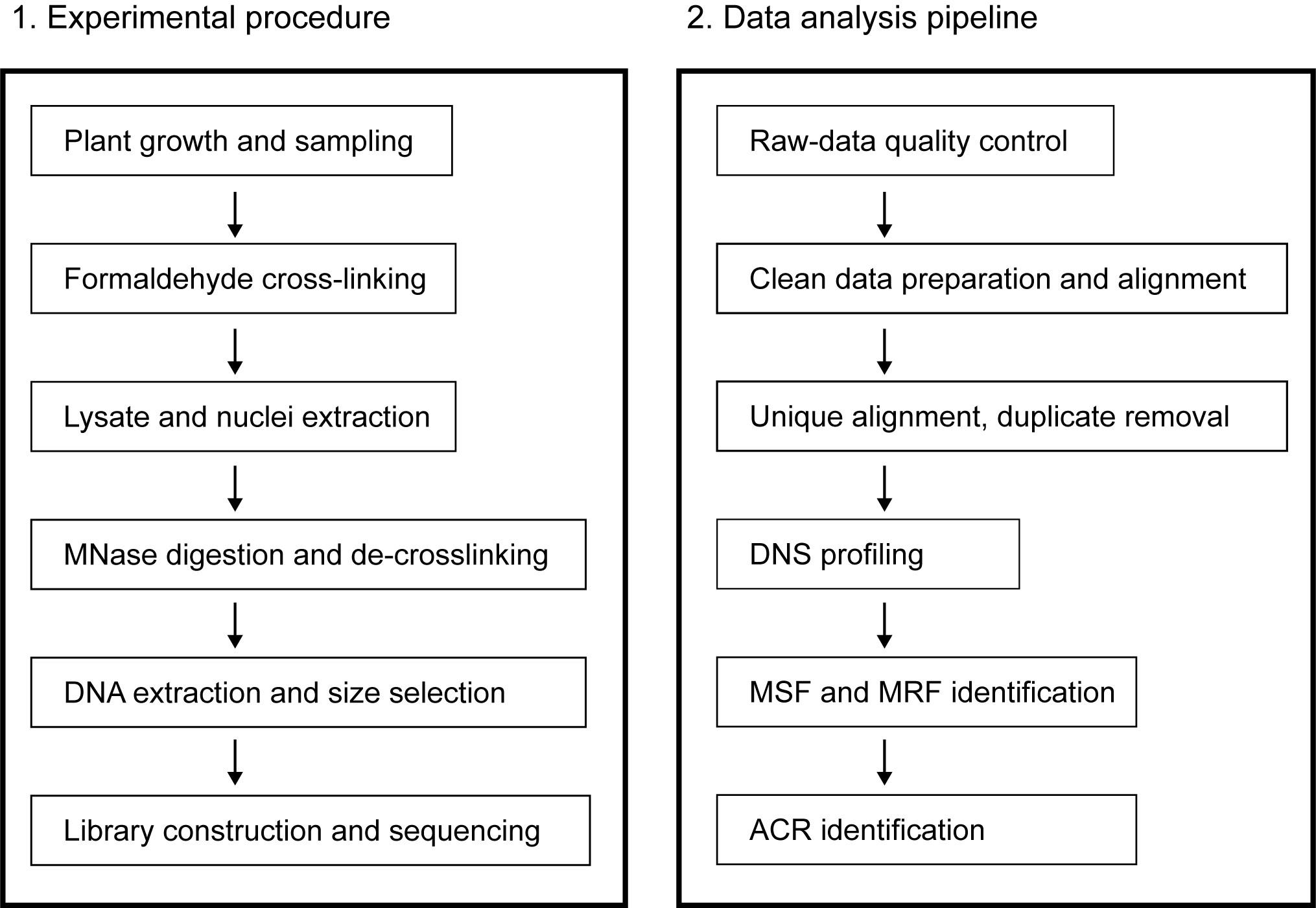
Figure 1. Schematic overview of the protocol.The experimental flow is shown on the left and the data analysis flow isshown on the right. MSF: MNase-sensitive footprint; MRF: MNase-resistantfootprint; ACR: accessible chromatin region.
Materials and reagents
Materials
Wheat seedlings at the three-leaf stage (Aikang58, CAAS)
Miracloth (Calbiochem, catalog number: 475855-1R)
50 mL centrifuge tube (Corning, catalog number: 430290)
5 mL pipette (Corning, catalog number: 4487)
PIPES (BBI, catalog number: A600719)
Sorbitol (BBI, catalog number: A610491)
EGTA (Millipore, catalog number: 324626)
DTT (Thermo Fisher, catalog number: R0861)
Spermine (Sigma-Aldrich, catalog number: S3256)
Spermidine (Sigma-Aldrich, catalog number: S2626)
37% Formaldehyde (Sigma-Aldrich, catalog number: 818708)
PMSF (Thermo Fisher, catalog number: 36978)
Glycine (Diamond, catalog number: A100167)
1 M Tris-HCl (pH 7.5) (Sangon, catalog number: B548124)
0.5 M EDTA (pH 8) (Sangon, catalog number: B540625)
Sucrose (Diamond, catalog number: A100335)
MgCl2 (Sigma-Aldrich, catalog number: M8266)
CaCl2 (Sigma-Aldrich, catalog number: C3306)
KCl (Sigma-Aldrich, catalog number: P9541)
NaCl (Sigma-Aldrich, catalog number: S3014)
SDS (Thermo Fisher, catalog number: 28364)
Phenol:Chloroform:Isoamyl alcohol 25:24:1 (Wako, catalog number: 311-90151)
RNase (Thermo Fisher, catalog number: EN0531)
Isopropanol (Sangon, catalog number: A507048)
1× TE buffer (Sangon, catalog number: B548106)
Glycerol (Diamond, catalog number: A100854)
Triton X-100 (Sigma-Aldrich, catalog number: T8787)
Percoll (GE, catalog number: 17-0891)
MNase (Thermo Fisher, catalog number: 88216)
Proteinase K (Solarbio, catalog number: 17-0891)
NEBNext UltraTM DNA Library Prep kit for Illumina (NEB, catalog number: E7645S)
Qiaex II gel extraction kit (Qiagen, catalog number: 20021)
Solutions
Nuclei isolation buffer (see Recipes)
Fixation buffer (see Recipes)
Percoll cushion solution (see Recipes)
MNase digestion buffer (see Recipes)
Recipes
Note: All concentrations listed are final concentrations.
Nuclei isolation buffer
15 mM PIPES (NaOH at pH 6.8)
0.32 M sorbitol
80 mM KCl
20 mM NaCl
0.5 mM EGTA
2 mM EDTA
1 mM DTT
0.15 mM spermine
0.5 mM spermidine
Fixation buffer
Nuclei isolation buffer, add 1% formaldehyde and 0.1 mM PMSF freshly
Percoll cushion solution
50% (vol/vol) Percoll in nuclei isolation buffer
MNase digestion buffer
50 mM Tris-HCl at pH 7.5
320 mM sucrose
4 mM MgCl2
1 mM CaCl2
Equipment
Mortar and pestle (Avantor, catalog number: HALDL55/1/G)
Beaker (30 mL) (PYREX, catalog number: 1000-30)
Magnetic stirrer (Thermo Fisher, catalog number: S194615)
Hybridization oven (Galanz, catalog number: P70J17L-V1)
4 °C centrifuge (Eppendorf, catalog number: 5804)
Nanodrop 2000 (Thermo Fisher, catalog number: 13-400-412)
Software
Deeptools v3.4.3 (Max Planck Institute for Immunobiology and Epigenetics; https://deeptools.readthedocs.io/en/latest/index.html) (February 2022)
Samtools v1.6 (Genome Research Limited; http://www.htslib.org/doc/samtools.html) (February 2022)
BEDTools v2.29.1 (University of Utah; https://bedtools.readthedocs.io/en/latest/content/bedtools-suite.html) (February 2022)
R v3.2.2 (Lucent Technologies; https://www.r-project.org/) (March 2022)
IGV v2.5.0 (University of California; http://software.broadinstitute.org/software/igv/) (March 2022)
Trimmomatic v0.36 (THE USADEL LAB; http://www.usadellab.org/cms/?page=trimmomatic) (February 2022)
Bowtie2 v2.3.4 (Johns Hopkins University; http://bowtie-bio.sourceforge.net/bowtie2/index.shtml) (February 2022)
FastQC v0.11.8 (Babraham Bioinformatics; https://www.bioinformatics.babraham.ac.uk/projects/fastqc/) (February 2022)
Procedure
Material fixation
Sampling: Harvest 10 g of leaves or roots (water rinsing) from the three-leaf-stage wheat seedlings after 21 days of seeds’ germination and immediately freeze the tissues in liquid nitrogen. Store at -80 °C.
Grinding: Ground the frozen materials under liquid nitrogen using a mortar and pestle (previously cooled with liquid nitrogen).
Fixation: Prepare 100 mL of pre-cooled fixation buffer in a beaker: add 2.78 mL of 37% formaldehyde to 1% and 102 μL of 100 mM PMSF to 0.1 mM. Pour the ground sample into the beaker and magnetically stir the sample for 10 min (100–200× g).
Termination: Stop the reaction by adding 6.87 mL of 2 M glycine stock to 125 mM and magnetically stir for another 5 min.
Nuclear extraction
Stirring: Slowly add 12 mL of 10% (vol/vol) Triton X-100 stock to 1%, gently agitate, and incubate for 10 min. Pre-cool the refrigerated centrifuge now.
Filter: Filter the solution into a beaker with two layers of Miracloth filter cloth and add 15 mL of Percoll cushion solution into a 50 mL centrifuge tube. Gently add 35 mL of the filtrate with a pipette on the top of the solution surface and ensure the liquid flows down along the tube wall without disturbing the boundary layer. Centrifuge at 3,000× g for 15 min at 4 °C (acceleration and deceleration should be slow) (see Note 1).
Transfer: The middle layer of the centrifuged Percoll filtrate contains the nuclei; transfer this layer to 50 mL centrifuge tubes (see Note 1) and add a 1-fold volume of MNase digestion buffer. Centrifuge at 2,000× g for 10 min at 4 °C.
Reconstitution: Re-dissolve the precipitate from each 35 mL in 2.5 mL of MNase digestion buffer and dispense the sample into five tubes with 500 μL each. Measure and record the DNA concentration by Nanodrop 2000 (approximately 50–150 ng/µL).
Microscopy: Observe the morphology of the nuclei with a fluorescence microscope. (The nuclei can be flash-frozen in liquid nitrogen and stored at -80 °C for up to one month.)
Digestion and de-crosslinking
Digestion: Thaw proteinase K, MNase, and five tubes of nuclei samples on ice (the nuclei can only be thawed once); then, treat two tube samples with 10 U/mL MNase (light), two tube samples with 100 U/mL MNase (heavy), and one tube sample as a control. Incubate all for 5 min at room temperature (see Note 2).
Termination: Add 10.2 μL of 0.5 M EGTA stock to 10 mM and vibrate the samples to stop the digestion reaction.
De-crosslinking: Add 57.5 μL of 10% SDS to 1% and 5.75 μL of 10 μg/μL proteinase K to 100 μg/mL, vibrate the samples, and incubate overnight in a 65 °C hybridization oven (>6.5 h).
Product extraction
DNA extraction: Add an equal volume of 600 μL of Phenol:Chloroform:Isoamyl alcohol 25:24:1 and mix thoroughly by inversion. Centrifuge at 12,000× g for 10 min at room temperature. Transfer the supernatant into new 1.5 tubes, add 5 μL of RNase to 40 μg/μL, mix by inverting, and incubate at 37 °C for 15 min. Add 400 μL of pre-cooled isopropanol and mix gently. Then, place tubes at -20 °C for 20 min to precipitate DNA. Pre-cool the centrifuge and centrifuge at 12,000× g for 10 min at 4 °C. Discard the supernatant, add 1 mL of 70% ethanol, mix by inverting, and wash twice. Dry the remaining ethanol for 20 min in a fume hood. Dissolve the precipitate in 30 μL of 1× TE buffer.
Fragment selection: Run 1% agarose gel (using single-color loading), select and extract the 100–200 bp DNA fragment (Figure 2, Note 2), and purify the DNA using the Qiaex II gel extraction kit.
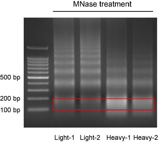
Figure 2. Ladders of MNase-digested DNA bands. The nuclei are treated with different concentrations of MNase and the DNA fraction from 100 to 200 bp is purified from the gel and sequenced.Library preparation and sequencing
Library construction: Construct the MNase-seq library using the NEBNext® UltraTM DNA Library Prep kit for Illumina® according to the instructions, where approximately 1 μg of total DNA is used.
High-throughput sequencing: Sequence the libraries on the Illumina platform HiSeq2000 system (or any Illumina sequencing instrument) to obtain 150 bp paired-end reads with 300 million reads (~90 G) for each sample of hexaploid wheat (genome size ~15 G) (see Note 3). Sequence the libraries for two biological replicates.
Data analysis
The analysis of arbitrary MNase-seq data can be achieved through the following instructions, with only minor modifications to the given code. Software used in this protocol can be easily installed via the conda command of anaconda ( https://www.anaconda.com/products/individual) or downloaded from the official website and installed by following the instructions. Make sure that the software is installed and the environment is set up normally in your Linux device before the program is executed.
Uploading data: Create a new working directory to store all the MNase-seq-related data and files and save all the raw data to a dedicated folder under that directory.
cd data1/user/path # enter your working directory
mkdir MNase_seq
cd MNase_seq
mkdir raw_data # move all your sequencing data to this directory
Quality control: Use FastQC to evaluate the quality of raw data obtained by sequencing, including basic statistics, base and sequence quality, GC content, sequence length distribution, adapter content, and other indicators of data.
mkdir ./fastqc_result
for i in ./raw_data/*.fq.gz
do
fastqc -o ./fastqc_result $i
done
Reads filtering: Use software such as Trimmomatic to filter the raw data to obtain clean data. The main goal of this step is to remove the adapter sequence, leading and trailing low-quality or N bases and sequences too short in length. When renaming the filtered data, tissue, digestion, and replicate should be considered. For example, “leaf_light_rep1” can be used to represent the first replicate with light digestion in leaves, and “root_heavy_rep2” can represent the second replicate with heavy digestion in roots.
mkdir clean_data
java -jar trimmomatic-0.36.jar PE -phred33 \
./raw_data/*.r1.fq.gz \
./raw_data/*.r2.fq.gz \
./clean_data/$name.1P.fq \
./clean_data/$name.1U.fq \
./clean_data/$name.2P.fq \
./clean_data/$name.2U.fq \
ILLUMINACLIP:data1/user/tools/Trimmomatic-0.36/adapters/\
TruSeq3-PE-2.fa:2:30:10:1:true \
LEADING:5 TRAILING:5 MINLEN:20 >trimmomatic.$name.log
Quality control: Use FastQC again to evaluate the quality of the clean data. If there is any undesirability, the parameters of the previous step can be adjusted and re-filtered until the reads can be used for the alignment in the next step.
for i in ./clean_data/*.fq.gz
do
fastqc -o ./fastqc_result $i
done
Sequence alignment: The filtered clean data is aligned to the reference genome using Bowtie2 software. Before that, library the genome with bowtie2-build and index the fasta file with Samtools faidx. Use the same parameters as suggested in maize for alignment.
bowtie2-build ref_genome.fa ref.genome
samtools faidx ref_genome.fa
bowtie2 --phred33 -p 10 --reorder -5 6 \
--no-mixed --no-discordant --no-unal --dovetail \
-x /index_path/ref.genome \
-1 ./$name.1P.fq \
-2 ./$name.2P.fq \
-S ./$name.sam >bowtie2.$name.log
Non-unique and duplicate alignments removal: Screen according to the MAPQ value in the alignment results. The larger the MAPQ value, the higher the confidence of the unique alignment. Here, we extract the part of MAPQ > 20. After that, remove the repeated reads due to PCR library amplification. Different software, like Picard, Sambamba, or Samtools, remove PCR duplicates. Here, we used Samtools markdup, before which the paired-end sequencing data were sorted by reads name and coordinates successively. A large index of the bam file should be established after that for the large genome.
function samtools_scripts(){
samtools view -q 20 -bhS $name.sam -o $name.Q20.bam
samtools sort -n $name.Q20.bam -o $name.Q20.nsort.bam
samtools fixmate -m $name.Q20.nsort.bam $name.Q20.nsort.ms.bam
samtools sort $name.Q20.nsort.ms.bam -o $name.Q20.ms.psort.bam
samtools markdup -r $name.Q20.ms.psort.bam $name.Q20.psort.markdup.bam
samtools index -c $name.Q20.psort.markdup.bam
}
samtools_scripts $name >samtools.$name.log
Differential nuclease sensitivity (DNS) identification: In the code here and later, we take “leaf_light_rep1” and “leaf_heavy_rep1” as examples for demonstration; you can replace the name when running other samples. The mapped reads of heavy digestion are subtracted from light digestion using bamCompare in the deepTools and are then normalized by the CPM method to output a DNS score file in bedgraph format. For this step, a 10-bp bin is used for division and statistics, and then a 50-bp window is used for smoothing.
bamCompare -b1 leaf_light_rep1.bam -b2 leaf_heavy_rep1.bam \
--scaleFactorsMethod None --normalizeUsing CPM --operation subtract \
--binSize 10 --smoothLength 50 --outFileFormat bedgraph \
-o leaf_diff_rep1.bdg
Bayes factor calculation: Here, reads coverage from both light-digested and heavy-digested samples is calculated, and the CPM method is used for standardizing; then, the Bayes factor is calculated for reads coverage in 10-bp intervals. You can speed up the program by running splitted files and calculating their Bayes values separately.
bamCoverage -b leaf_light_rep1.bam \
--binSize 10 --smoothLength 50 \
--normalizeUsing CPM --outFileFormat bedgraph \
-o leaf_light_rep1.bdg
bamCoverage -b leaf_heavy_rep1.bam \
--binSize 10 --smoothLength 50 \
--normalizeUsing CPM --outFileFormat bedgraph \
-o leaf_heavy_rep1.bdg
bedtools unionbedg \
-i leaf_light_rep1.bdg leaf_heavy_rep1.bdg \
-header -names light heavy \
>leaf_rep1.unionbdg
# run the R script to obtain a file named “leaf_rep1.unionbdg.bayes”
Rscript bayes_factor_caculator.R leaf_rep1.unionbdg
Accessible chromatin regions identification: Based on the Bayes values in the “leaf_rep1.unionbdg.bayes” file, identify MNase-sensitive footprints (MSFs) and MNase-resistant footprints (MRFs) in the “leaf_diff_rep1.bdg” file. Parts with DNS values greater than 0 and Bayes values greater than 0.5 are defined as significant MSFs; parts with DNS values lower than 0 and Bayes values greater than 0.5 are defined as significant MRFs (see Note 4). The significant MSF or MRF signals within 200 bp are merged into one MSF or MRF signal. The significant MSFs are also referred to as MNase-hypersensitive (MNase HS) regions or ACRs (see Note 5).
bedtools unionbedg \
-i leaf_diff_rep1.bdg leaf_rep1.unionbdg.bayes \
>leaf.diff_rep1_bayes
cat leaf.diff_rep1_bayes | awk '$4>0 && $5>0.5' | \
cut -f1-3 | bedtools merge -d 200 \
>leaf.MSF_rep1_bayes_0.5_merge_200.bed
cat leaf.diff_rep1_bayes | awk '$4<0 && $5>0.5' | \
cut -f1-3 | bedtools merge -d 200 \
>leaf.MRF_rep1_bayes_0.5_merge_200.bed
Signal visualization: The reads coverage depth of the samples obtained by different digestion treatments and the sensitivity imprint DNS values can be generated with bigwig files by deepTools and then loaded into the Integrative Genomics Viewer (IGV browser) for browsing. The MSF or MRF location files can also be loaded into the IGV browser.
bamCoverage -b leaf_light_rep1.bam \
--binSize 10 --smoothLength 50 \
--normalizeUsing CPM --outFileFormat bigwig \
-o leaf_light_rep1.bw
bamCoverage -b leaf_heavy_rep1.bam \
--binSize 10 --smoothLength 50 \
--normalizeUsing CPM --outFileFormat bigwig \
-o leaf_heavy_rep1.bw
bamCompare -b1 leaf_light_rep1.bam -b2 leaf_heavy_rep1.bam \
--scaleFactorsMethod None --normalizeUsing CPM --operation subtract \
--binSize 10 --smoothLength 50 --outFileFormat bigwig \
-o leaf_diff_rep1.bw
Attached R script for calculating Bayes factor: Upload the script to the same folder as “leaf_rep1.unionbdg” before use and then modify the working path, nh, nf, and other assignments according to your experiment.
### bayes factor caculator 1.0 ###
setwd("data1/user/path/MNase_seq")
M=100000
nh=2
nf=2
bayes_factor_caculator <- function(old, new) {
lkd.model1=function(y,n,lambda){ return(exp(-n*lambda+y*log(lambda))) }
lkd.model2=function(y1,n1,y2,n2,lambda1,lambda2){ return(exp(-n1*lambda1+y1*log(lambda1)-n2*lambda2+y2*log(lambda2))) }
BF_MC=function(a,b,y1,n1,y2,n2,M){
lambda1=rgamma(M,a,b)
m1=cumsum(lkd.model1(y1+y2,n1+n2,lambda1))/(1:M)
lambda2.1=rgamma(M,a,b)
lambda2.2=rgamma(M,a,b)
m2=cumsum(lkd.model2(y1,n1,y2,n2,lambda2.1,lambda2.2))/(1:M)
return(m2/m1)
}
con <- file(old,"rt")
line <- readLines(con,n=1)
while (length(line) > 0){
line <- unlist(strsplit(line,split = "\t"))
qh <- as.numeric(line[5])
qf <- as.numeric(line[4])
set.seed(1)
bayes <- BF_MC(10,1,qh,nh,qf,nf,M)[M]
newline=t(c(line[1],line[2],line[3],round(bayes,5)))
write.table(newline, new, col.names = F, row.names = F, sep = '\t', quote=F, append =T)
line <- readLines(con, n = 1)
}
close(con)
# BF_MC(10,1,qh,nh,qf,nf,M)[M]
# qh: total number of mapped reads for heavy-digestion
# nh: number of replicates for heavy-digestion
# qf: total number of mapped reads for light-digestion
# nf: number of replicates for light-digestion
}
args=commandArgs(T)
bayes_factor_caculator(args[1], paste0(args[1], '.bayes'))
Notes
Care should be taken when adding the filtrate to the Percoll cushion, slowly adding the filtrate along the top of the tube wall without causing violent fluctuations in the interface and mixing between liquids. When centrifuging, acceleration and deceleration must be slow. After centrifugation, a cloudy layer of liquid containing the nuclei at the interface between Percoll and the filtrate should be taken out, rather than the precipitation at the bottom of the centrifuge tube.
The timing of MNase and EGTA addition during the digestion reaction should be precisely controlled. Furthermore, the selection of the 100–200 bp fragment should be precise and consistent among different samples and replicates.
We recommend sequencing the library samples using PE150, in which case each fragment can be fully read. The sequencing depth can be determined according to the size of the genome, where the coverage of 6× is used for wheat, and the final actual performance is good. In a specific implementation, a portion of data can be preliminarily measured, and then the amount of deep sequencing data could be determined according to the effect.
When identifying significant MSF and MRF, if the background signal is too high, the threshold of the Bayes factor can be raised or the signals with too short length can be filtered directly to obtain more real and effective signals, which can be adjusted repeatedly in combination with the actual display of IGV browser.
While doing MNase-seq, we recommend performing ChIP-seq of histone modifications, such as activation modification H3K9ac, which are significant features of some ACRs and have good colocalization with ACR signals, which can be used to assist with the identification.
Acknowledgments
This protocol was applied in our open chromatin study in wheat (Kong et al., 2024), which was supported by the Central Public-interest Scientific Institution Basal Research Fund (Y2021YJ01), the National Natural Science Foundation of China (Major Program, 31991213), and the National Natural Science Foundation of China (31971882). We mainly referred to open chromatin research articles in maize (Vera et al., 2014; Rodgers-Melnick et al., 2016). In the development of this procedure, we received help from Eli Rodgers-Melnick and Daniel L. Vera. Professor Zou Cheng at Cornell University helped with our algorithms. Thanks a lot for their help!
Competing interests
There are no conflicts of interest or competing interests.
References
- Brahma, S. and Henikoff, S. (2019). RSC-Associated Subnucleosomes Define MNase-Sensitive Promoters in Yeast. Mol. Cell. 73(2): 238-249.e3.
- Chereji, R. V., Ocampo, J. and Clark, D. J. (2017). MNase-Sensitive Complexes in Yeast: Nucleosomes and Non-histone Barriers. Mol. Cell. 65(3): 565-577.e3.
- Cook, A., Mieczkowski, J. and Tolstorukov, M. Y. (2017). Single-Assay Profiling of Nucleosome Occupancy and Chromatin Accessibility. Curr. Protoc. Mol. Biol. 120, 21 34 21-21 34 18.
- Fang, Y., Wang, X., Wang, L., Pan, X., Xiao, J., Wang, X. E., Wu, Y. and Zhang, W. (2016). Functional characterization of open chromatin in bidirectional promoters of rice. Sci. Rep. 6: 32088.
- Jordan, K. W., He, F., de Soto, M. F., Akhunova, A. and Akhunov, E. (2020). Differential chromatin accessibility landscape reveals structural and functional features of the allopolyploid wheat chromosomes. Genome. Biol. 21(1): 176.
- Klein, D. C. and Hainer, S. J. (2020). Genomic methods in profiling DNA accessibility and factor localization. Chromosome. Res. 28(1): 69-85.
- Lu, Z., Marand, A. P., Ricci, W. A., Ethridge, C. L., Zhang, X. and Schmitz, R. J. (2019). The prevalence, evolution and chromatin signatures of plant regulatory elements. Nat. Plants. 5(12): 1250-1259.
- Mieczkowski, J., Cook, A., Bowman, S. K., Mueller, B., Alver, B. H., Kundu, S., Deaton, A. M., Urban, J. A., Larschan, E., Park, P. J., et al. (2016). MNase titration reveals differences between nucleosome occupancy and chromatin accessibility. Nat. Commun. 7: 11485.
- Rodgers-Melnick, E., Vera, D. L., Bass, H. W. and Buckler, E. S. (2016). Open chromatin reveals the functional maize genome. Proc. Natl. Acad. Sci. U S A. 113(22): E3177-3184.
- Schwartz, U., Nemeth, A., Diermeier, S., Exler, J. H., Hansch, S., Maldonado, R., Heizinger, L., Merkl, R. and Langst, G. (2019). Characterizing the nuclease accessibility of DNA in human cells to map higher order structures of chromatin. Nucleic. Acids. Res. 47: 1239-1254.
- Tsompana, M. and Buck, M. J. (2014). Chromatin accessibility: a window into the genome. Epigenet. Chromatin. 7(1): 33.
- Vera, D. L., Madzima, T. F., Labonne, J. D., Alam, M. P., Hoffman, G. G., Girimurugan, S. B., Zhang, J., McGinnis, K. M., Dennis, J. H. and Bass, H. W. (2014). Differential nuclease sensitivity profiling of chromatin reveals biochemical footprints coupled to gene expression and functional DNA elements in maize. Plant. Cell. 26(10): 3883-3893.
- Yan, W., Chen, D., Schumacher, J., Durantini, D., Engelhorn, J., Chen, M., Carles, C. C. and Kaufmann, K. (2019). Dynamic control of enhancer activity drives stage-specific gene expression during flower morphogenesis. Nat. Commun. 10(1): 1705.
- Zhao, H., Zhang, W., Zhang, T., Lin, Y., Hu, Y., Fang, C., and Jiang, J. (2020). Genome-wide MNase hypersensitivity assay unveils distinct classes of open chromatin associated with H3K27me3 and DNA methylation in Arabidopsis thaliana. Genome. Biol. 21(1): 24.
Supplementary information
- Data and code availability: All data and code have been deposited to GitHub: https://github.com/Bio-protocol/ACRs_by_MNase-seq.
Article Information
Copyright
© 2024 The Author(s); This is an open access article under the CC BY-NC license (https://creativecommons.org/licenses/by-nc/4.0/).
How to cite
Category
Plant Science > Plant molecular biology > DNA
Molecular Biology > DNA > Chromatin accessibility
Do you have any questions about this protocol?
Post your question to gather feedback from the community. We will also invite the authors of this article to respond.
![]() Tips for asking effective questions
Tips for asking effective questions
+ Description
Write a detailed description. Include all information that will help others answer your question including experimental processes, conditions, and relevant images.