Computational Analysis of Maize Enhancer Regulatory Elements Using ATAC-STARR-seq

Alexandre P. Marand

doi:10.21769/BioProtoc.4953

Improve Research Reproducibility A Bio-protocol resource

Submit a Protocol
Receive Our Alerts
Log in
/
Sign up
- My Bio Page
- Edit My Profile
- Change Password
- Log Out
EN
- EN - English
- CN - 中文

Peer-reviewed

Computational Analysis of Maize Enhancer Regulatory Elements Using ATAC-STARR-seq

AM Alexandre P. Marand email

Published: Mar 5, 2024 DOI: 10.21769/BioProtoc.4953 Views: 340

Reviewed by: G. Alex MasonPrashanth N Suravajhala

PDF

Ask a question

How to cite

Favorite

Cited by

Protocol Collections

Cell Imaging - A Special Collection for Cell Bio 2023

See all

Abstract

The blueprints for development, response to the environment, and cellularfunction are largely the manifestation of distinct gene expression programscontrolled by the spatiotemporal activity of cis-regulatory elements. Althoughbiochemical methods for identifying accessible chromatin—a hallmark ofactive cis-regulatory elements—have been developed, approaches capable ofmeasuring and quantifying cis-regulatory activity are only beginning to berealized. Massively parallel reporter assays coupled to chromatin accessibilityprofiling present a high-throughput solution for testing thetranscription-activating capacity of millions of putatively regulatory DNAsequences in parallel. However, clear computational pipelines for analyzingthese high-throughput sequencing-based reporter assays are lacking. In thisprotocol, I layout and rationalize a computational framework for the processingand analysis of the transposase accessible chromatin profiling followed byself-transcribed active regulatory region sequencing (ATAC-STARR-seq) data froma recent study in Zea mays. The approach described herein canbe adapted to other sequencing-based reporter assays and is largely modelorganism–agnostic with appropriate input substitutions.

Keywords: STARR-seq

ATAC-seq

ATAC-STARR-seq

Regulatory activity

cis-regulatory elements

Accessible chromatin

Transcriptional regulation

Enhancers

Background

Eukaryotic cells exhibit remarkable functional and morphological diversity despite containing a generally invariant copy of the same genomic sequence. Cellular heterogeneity arises in part due to the activities of cis-regulatory elements (CREs), short DNA-binding motifs recognized by sequence-specific transcription factors (TFs). CREs are often found in clusters termed cis-regulatory modules (CRMs) that dictate highly dynamic spatiotemporal patterns of gene expression via the cooperative activities of DNA-bound TFs (Schmitz et al., 2022). For proper activation of transcription, the cell strictly regulates CRM activity by controlling TF access of CRM sequences through nucleosome dynamics. Genome-wide approaches, such as the assay for transposase accessible chromatin sequencing (ATAC-seq), have been developed to profile accessible chromatin regions (ACRs) (Buenrostro et al., 2013; Minnoye et al., 2021). In general, CRMs that localize to accessible chromatin reflect active regulatory elements (Marand et al., 2017; Schmitz et al., 2022). Thus, activation and silencing of gene expression is effectively controlled by the relative chromatin accessibility of cognate CRMs.

CREs can be classified into distinct functional groups based on their regulatory effect on transcription, including enhancers, silencers, promoters, and insulators (Schmitz et al., 2022). Of these, enhancers are of particular interest due to their transcription-activating properties that function independently of location and orientation of their target genes, in contrast to the stereotypical locations of promoters surrounding gene transcription start sites (TSSs) (Marand et al., 2017; Schmitz et al., 2022). While analysis of chromatin accessibility in distinct tissues and cell types has been central to the identification of CRMs (Marand et al., 2021), chromatin profiling techniques are largely qualitative and lack the ability to quantitatively estimate regulatory activity. To overcome these challenges, massively parallel reporter assays (MPRAs) have been developed to quantify the transcription-activating properties of diverse sequences (Melnikov et al., 2012; Arnold et al., 2013). In particular, self-transcribing active regulatory region sequencing (STARR-seq) demonstrates the greatest potential for broad application by eliminating the need for homogenous cell lines available only in mammalian models typical of other MPRA methods (Arnold et al., 2013; Ricci et al., 2019; Sun et al., 2019; Jores et al., 2020). Although STARR-seq was originally designed to profile the entire genome for regulatory activity, recent implementations have successfully utilized ATAC-seq libraries as input (ATAC-STARR-seq), reducing the search space to potential regulatory regions and offsetting sequencing costs and library complexity requirements (Figure 1). Despite its promise as a powerful approach towards understanding cis-regulatory activity, computational analysis of ATAC-STARR-seq data remains challenging, particularly due to a lack of dedicated software and computational pipelines.

Here, I present a computational pipeline for analysis of ATAC-STARR-seq data generated in Zea mays L., cultivar B73 (Ricci et al., 2019). After processing and evaluation of data quality, I demonstrate how ATAC-STARR-seq data analysis allows for the interrogation of new biological questions. The pipeline can be run entirely from the code below or through freely available bash, perl, and R scripts hosted at https://github.com/Bio-protocol/Maize_ATAC_STARR_seq.

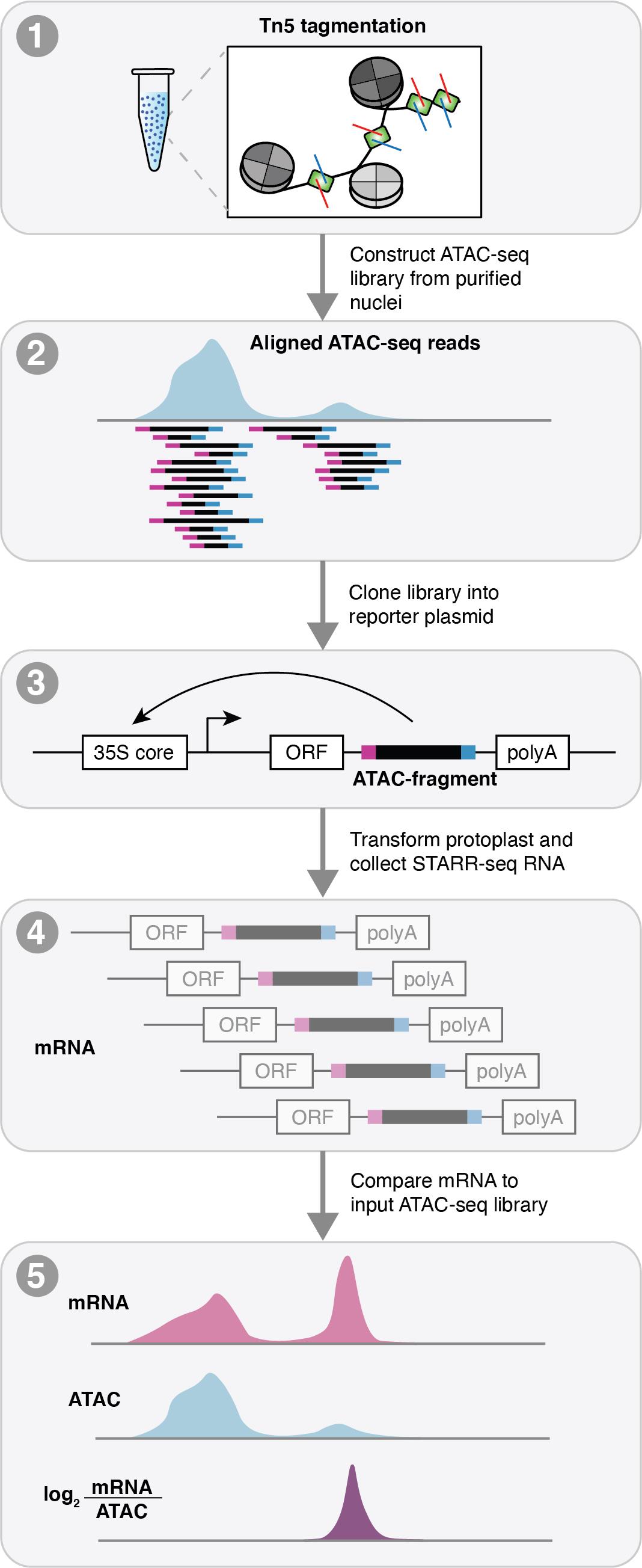
Figure 1. Schematic of assay for transposase accessible chromatin profiling followed by self-transcribed active regulatory region sequencing (ATAC-STARR-seq). ATAC-STARR-seq begins by first generating an ATAC-seq library. The ATAC fragments are then cloned into a reporter assay and transformed into maize protoplasts. Transformed protoplasts are then split into two pools: the first for sequencing the input fragments (ATAC-seq DNA) and the second for purifying transcribed (mRNA) ATAC-seq fragments that facilitate their own transcription from the reporter construct. Raw sequenced reads for the ATAC-seq input and mRNA output are processed and aligned to the maize reference genome and compared to provide estimates of cis-regulatory activity.

Equipment

This pipeline assumes that a user has knowledge of shell commands and is comfortable working on a Linux-based operating system.

Computational requirements
The following procedure can be run on any Linux-like system. However, this protocol and publicly available code is written for executing commands via a high-performance computing (HPC) cluster managed by a SLURM scheduler. Still, the code presented here can be readily converted to TORQUE or other HPC systems. The pipeline assumes a working Perl interpreter version 5.30.0 or greater and R version 3.6.2 or greater.

Software

The following analytical procedure makes use of several standard computational tools that are assumed to be available in the user’s shell environment:

BWA MEM (Li and Durbin, 2009) v0.7.17; http://bio-bwa.sourceforge.net/bwa.shtml
SAMtools (Li et al., 2009) v1.14; http://www.htslib.org
BEDtools (Quinlan and Hall, 2010) v2.27.1; https://bedtools.readthedocs.io/en/latest/
SRA-toolkit (Leinonen et al., 2011) v2.11.1; https://github.com/ncbi/sra-tools
fastp (Chen et al., 2018) v0.20.0; https://github.com/OpenGene/fastp
pigz v2.4; https://zlib.net/pigz/
MACS2 (Liu, 2014) v2.2.7.1; https://pypi.org/project/MACS2/
UCSC binaries (Kent et al., 2010) v1.04.0; http://hgdownload.soe.ucsc.edu/admin/exe/linux.x86_64/
tabix (Li, 2011) v0.2.6; http://www.htslib.org/doc/tabix.html
IGV (Thorvaldsdottir et al., 2013) v2.11.1; https://software.broadinstitute.org/software/igv
MEME (Grant et al., 2011) v5.4.1; https://meme-suite.org/meme/index.html
CrossMap (Zhao et al., 2014) v0.5.1; http://crossmap.sourceforge.net/
DeepTools (Ramirez et al., 2014) v3.5.1; https://deeptools.readthedocs.io/en/develop/index.html

Input data

The starting input for this computational pipeline uses paired-end sequencing data from an ATAC-STARR-seq experiment performed on maize protoplasts (Ricci et al., 2019). The ATAC-STARR-seq experiment consisted of a DNA input (ATAC-seq library) and a mRNA readout (self-transcribed regulatory regions) to identify genomic regions exhibiting transcription-activating regulatory activity.

Transfected ATAC-seq DNA-input FASTQ
Transcribed ATAC-seq mRNA FASTQ

Procedure

An overview of the ATAC-STARR-seq pipeline is presented in Figure 2.

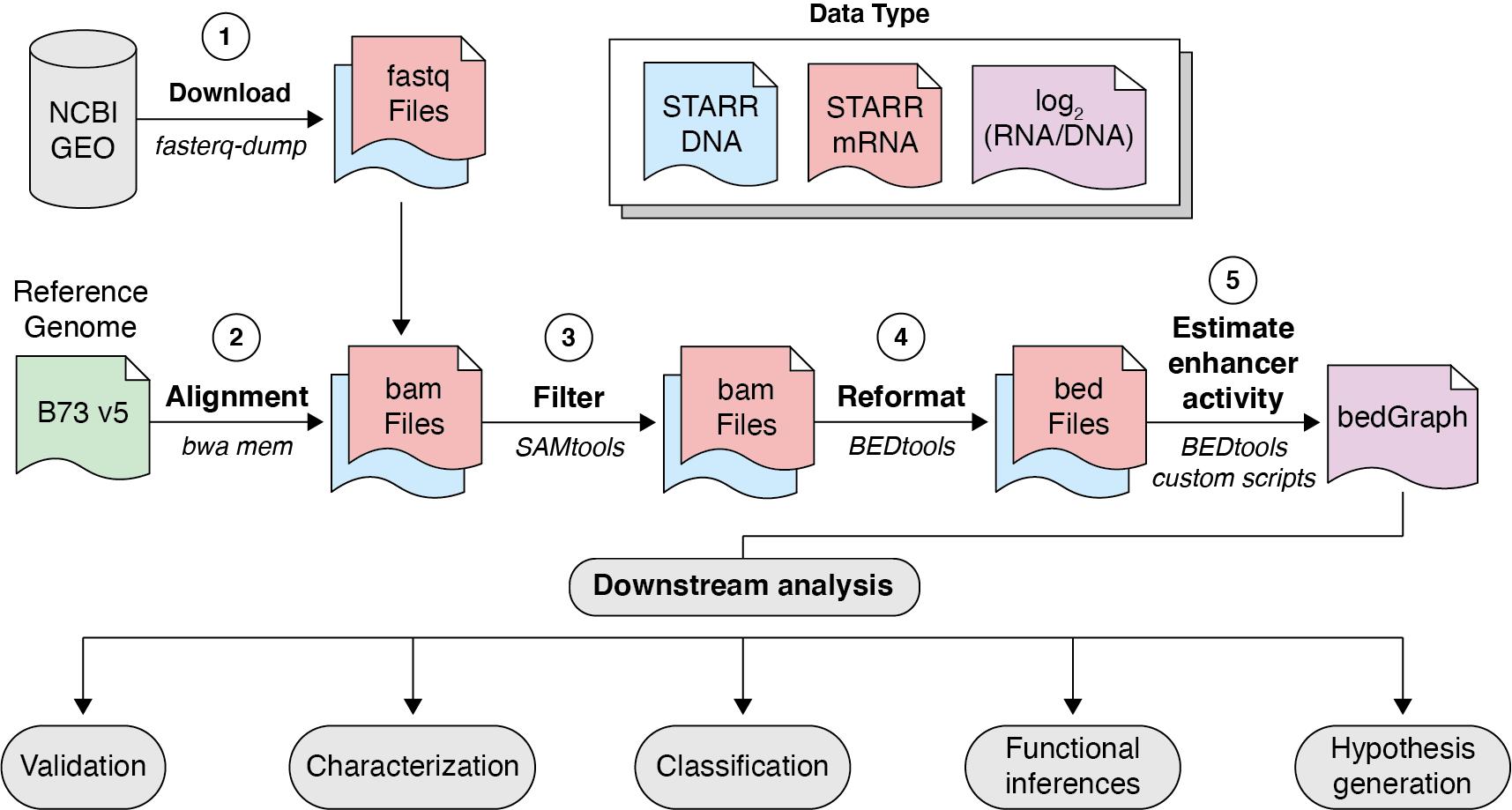
Figure 2. Computational workflow for the assay for transposase accessible chromatin profiling followed by self-transcribed active regulatory region sequencing (ATAC-STARR-seq) data. Raw sequence ATAC-STARR-seq data are first acquired from NCBI GEO, processed, and aligned to the reference genome with BWA MEM, filtered via SAMtools, reformatted as fragments with BEDtools, and compared via BEDtools and custom R scripts to provide estimates of enhancer activity for downstream analysis.

Download and prepare the requisite data and reference genome sequence
1. Raw mRNA ATAC-STARR-seq data generated from transfection of Zea mays leaf ATAC-seq fragments in Z. mays protoplasts, and the accompanying ATAC-seq input fragments, are publicly available on NCBI GEO. ATAC-STARR-seq mRNA and DNA input can be downloaded with fasterq-dump available from the SRA-toolkit package:
  
  # set variables and download FASTQ files
  mkdir FASTQ_files
  cd FASTQ_files
  fasterq-dump -o B73_maize_DNA_input.fastq SRR10964904
  fasterq-dump -o B73_maize_mRNA_output.fastq SRR10964905
2. To save disk space, we will compress the FASTQ files with pigz. By default, pigz uses all available processors or eight if the number of available processors is unknown. Alternatively, users can use the unix tool, gzip, to compress the STARR mRNA and ATAC input DNA FASTQ files.
  
  # compress fastq files
  pigz *.fastq
  
  # NOT RUN
  # Tip: gzip can be used as an alternative to pigz (parallel gzip)
  # gzip *.fastq
3. Download the B73 reference genome sequence and gene annotation. The original article mapped raw reads to version 4 of the B73 maize reference genome. In this case study, I map and analyze maize ATAC-STARR-seq data to version 5 of the B73 maize reference genome to showcase how updated reference genomes and read mapping strategies enable informative reanalysis of publicly available data sets (Hufford et al., 2021).
  
  # download reference data
  cd ../
  mkdir Genome_Reference
  cd Genome_Reference
  wget https://download.maizegdb.org/Zm-B73-REFERENCE-NAM-5.0/Zm-B73-REFERENCE-NAM-5.0.fa.gz
  wget https://download.maizegdb.org/Zm-B73-REFERENCE-NAM-5.0/Zm-B73-REFERENCE-NAM-5.0_Zm00001eb.1.gff3.gz
4. To map data to the reference genome, we first need to decompress the FASTA file. Constructing reference genome indices is a prerequisite for BWA alignment and allows for faster post-alignment processing of BAM/SAM/BED formatted files with command line tools such as SAMtools and BEDtools.
  
  # create indices for reference genome FASTA
  gunzip Zm-B73-REFERENCE-NAM-5.0.fa.gz
  samtools faidx Zm-B73-REFERENCE-NAM-5.0.fa
  bwa index Zm-B73-REFERENCE-NAM-5.0.fa
Trim adapters and remove low quality reads
1. Illumina platforms may produce reads with adapter sequences on the 3’ ends if the DNA insert is shorter than the number of cycles. Additionally, the fidelity of sequencing by synthesis deteriorates with each additional cycle due to phasing, the desynchronization of cycles that results from unremoved terminator caps ultimately leading to greater uncertainty of base calls in later cycles. Removing adapter contamination and low-quality bases increases the total number of alignable reads, particularly important when analyzing a relatively lower sequence complexity experiment, such as ATAC-STARR-seq. We will use fastp to remove sequencing adapters and low-quality reads for the mRNA output and DNA input. A script to perform read trimming can be found here: https://github.com/Bio-protocol/Maize_ATAC_STARR_seq/blob/master/workflow/step01_trim_raw_reads.sh
  
  # set variables
  cd ../
  fastqdir=$PWD/FASTQ_files
  dna=B73_maize_DNA_input
  rna=B73_maize_mRNA_output
  threads=16
  
  # trim and filter DNA input reads
  fastp -j $dna.json -h $dna.html -w $threads \
  -i $fastqdir/${dna}_1.fastq.gz -I $fastqdir/${dna}_2.fastq.gz \
  -o $fastqdir/${dna}_1.trim.fastq.gz -O $fastqdir/${dna}_2.trim.fastq.gz
  
  # trim and filter mRNA output reads
  fastp -j $rna.json -h $rna.html -w $threads \
  -i $fastqdir/${rna}_1.fastq.gz -I $fastqdir/${rna}_2.fastq.gz \
  -o $fastqdir/${rna}_1.trim.fastq.gz -O $fastqdir/${rna}_2.trim.fastq.gzbS - | samtools sort - > $outdir/B73_maize_mRNA_output.raw.bam
  
  # tidy up log files
  mkdir fastp_log_files
  mv *.json *.html fastp_log_files
Align and process sequenced reads
1. After trimming and quality filtering reads, we align the input DNA and output mRNA reads to the maize B73 version 5 reference genome. To speed up the alignment and downstream processing, we are using 24 CPUs (-t 24) to align the input and output reads. However, users should modify this value to reflect the number of available cores on their system. Additionally, we mark split hits as secondary alignments (-M) to be filtered out downstream, as the maize genome is highly repetitive. The output of BWA MEM is piped to SAMtools view for compression (SAM to BAM) and sorted by alignment coordinate prior to further processing to minimize the footprint on disk. A script to perform these steps can be found here: https://github.com/Bio-protocol/Maize_ATAC_STARR_seq/blob/master/workflow/step02_align_STARR_data.sh
  
  cd ../
  mkdir BAM_files
  outdir=$PWD/BAM_files
  refdir=$PWD/Genome_Reference
  fastqdir=$PWD/FASTQ_files
  
  # align DNA input and pipe to samtools for SAM to BAM conversion
  bwa mem -M -t 24 $refdir/Zm-B73-REFERENCE-NAM-5.0.fa $fastqdir/B73_maize_DNA_input_1.trim.fastq.gz $fastqdir/B73_maize_DNA_input_2.trim.fastq.gz | samtools view -bS - | samtools sort - > $outdir/B73_maize_DNA_input.raw.bam
  
  # align RNA output and pipe to samtools for SAM to BAM conversion
  bwa mem -M -t 24 $refdir/Zm-B73-REFERENCE-NAM-5.0.fa $fastqdir/B73_maize_mRNA_output_1.trim.fastq.gz $fastqdir/B73_maize_mRNA_output_2.trim.fastq.gz | samtools view -bS - | samtools sort - > $outdir/B73_maize_mRNA_output.raw.bam
2. To ensure that only high-quality alignments remain, here we remove non-properly paired reads (-f 3), secondary hits (-F 256), alignments with low mapping quality (-q 10), and multiple mapped reads (grep -v -E -e '\bXA:Z:’) using a combination of SAMtools and unix commands. The header, which contains information on the reference genome and the read mapping parameters, is retained in the output by setting the -h flag in the SAMtools view command.
  
  # filter DNA input alignments
  samtools view -h -q 10 -f 3 -F 256 $outdir/B73_maize_DNA_input.raw.bam
  | grep -v -E -e '\bXA:Z:' | samtools view -bSh - > $outdir/B73_maize_DNA_input.mq10.pp.unique.bam
  
  # filter mRNA output alignments
  samtools view -h -q 10 -f 3 -F 256 $outdir/B73_maize_ mRNA_output.raw.bam
  | grep -v -E -e '\bXA:Z:' | samtools view -bSh - > $outdir/B73_maize_mRNA_output.mq10.pp.unique.bam
3. A major difference between analysis of ATAC-seq and STARR-seq data is how assay information is captured by sequencing. For paired-end ATAC-seq, since Tn5 inserts sequencing adapters adjacent to its bound genomic location, chromatin accessibility is encoded as the 5’ ends of sequenced reads. In contrast, STARR-seq produces mRNA transcripts from fragments that are capable of activating their own transcription; thus, the entire STARR-seq mRNA and DNA fragment is informative for analysis. The following commands extract the coordinates of sequenced fragments by leveraging the CIGAR strings in BAM paired-end alignments for DNA input and mRNA output. A script to extract fragments can be found here: https://github.com/Bio-protocol/Maize_ATAC_STARR_seq/blob/master/workflow/step03_extract_fragments.sh
  
  # create output directory
  mkdir BED_files
  
  # variables
  outdir=$PWD/BAM_files
  beddir=$PWD/BED_files
  dna=B73_maize_DNA_input
  rna=B73_maize_mRNA_output
  
  # extract DNA input fragments (ignore the warnings from bedtools with respect to “missing” mate pairs, these reflect one of the pairs that had its mate filtered in prior steps)
  echo " extracting fragments from STARR DNA input ..."
  samtools sort -n $outdir/$dna.mq10.pp.unique.bam \
  | bedtools bamtobed -bedpe -i - \
  | sort -k1,1 -k2,2n - \
  | cut -f1,2,6 - > $beddir/$dna.fragments.bed
  
  # extract mRNA output fragments
  echo " extracting fragments from STARR mRNA output ..."
  samtools sort -n $outdir/$rna.mq10.pp.unique.bam \
  | bedtools bamtobed -bedpe -i - \
  | sort -k1,1 -k2,2n - \
  | cut -f1,2,6 - > $beddir/$rna.fragments.bed
Identify regions with enriched activity over background
1. To identify regions of the genome with the capacity to activate transcription, we assess enrichment of mRNA reads relative to the input ATAC-seq fragments using MACS2. As MACS2 is a general peak caller, we need to adjust the default settings to tailor the analysis specifically for ATAC-STARR-seq data. Since this experiment did not use unique molecular identifiers, and the number of transcripts from fragment is a direct reflection of its regulatory activity, duplicate mRNA fragments are retained (--keep-dup all). To directly use coverages determined by the input fragment coordinates, we turn off the default fragment shifting model (--nomodel) and set the input type to BEDPE (-f BEDPE). Additionally, we reduce the maximum gap size between candidate peaks to allow for the identification of fine-mapped regulatory elements within a broader regulatory region (--max-gap 50) by setting the minimum peak size to 300 (--min-length 300). Finally, we use the background coverage rates in place of the local bias, which aids in peak detection (--nolambda). A script to perform peak calling can be found here: https://github.com/Bio-protocol/Maize_ATAC_STARR_seq/blob/master/workflow/step04_call_peaks.sh
  
  # prepare output directory and input files
  mkdir Peak_data
  
  # generate input files
  uniq $beddir/$rna.fragments.bed > $beddir/$rna.fragments.uniq.bed
  uniq $beddir/$dna.fragments.bed > $beddir/$dna.fragments.uniq.bed
  cat $beddir/$rna.fragments.uniq.bed $beddir/$dna.fragments.uniq.bed | sort -k1,1 -k2,2n - > $beddir/ALL.fragments.uniq.bed
  
  # find regulatory regions
  echo " calling regulatory regions without duplicate removal ..."
  macs2 callpeak -t $beddir/$rna.fragments.bed \
  -c $beddir/ALL.fragments.uniq.bed \
  --keep-dup all \
  --max-gap 50 \
  --min-length 300 \
  --nolambda \
  --nomodel \
  -f BEDPE \
  -g 1.6e9 \
  --bdg \
  -n STARR_wdups
  
  # find regulatory regions
  echo " calling regulatory regions with duplicate removal ..."
  macs2 callpeak -t $beddir/$rna.fragments.uniq.bed \
  -c $beddir/$dna.fragments.uniq.bed \
  --keep-dup all \
  --max-gap 50 \
  --min-length 300 \
  --nolambda \
  --nomodel \
  -f BEDPE \
  -g 1.6e9 \
  --bdg \
  -n STARR_nodups
  
  # find regulatory regions using all unique fragments
  echo " calling regulatory regions by aggregating all unique fragments ..."
  macs2 callpeak -t $beddir/ALL.fragments.uniq.bed \
  --keep-dup all \
  --max-gap 50 \
  --min-length 300 \
  --nolambda \
  --nomodel \
  -f BEDPE \
  -g 1.69e9 \
  --bdg \
  -n STARR_ALL
  
  # clean-up output
  mv STARR_* Peak_data
  
  # merge peaks
  cd Peak_data
  cat STARR_wdups_peaks.narrowPeak STARR_nodups_peaks.narrowPeak STARR_ALL_peaks.narrowPeak | sort -k1,1 -k2,2n - | bedtools merge -i - > STARR_merged_peaks.bed
2. To estimate regulatory activity at fine scale, first we need to create a list of unique intervals based on mRNA and DNA fragments. Next, we count the intersection of mRNA and DNA fragments for each unique interval. Finally, we remove all the temporary files to reduce the footprint on disk. A script to estimate enhancer activity can be found here: https://github.com/Bio-protocol/Maize_ATAC_STARR_seq/blob/master/workflow/step05_estimate_enhancer_activity.sh
  
  # variables
  beddir=$PWD/BED_files
  dna=B73_maize_DNA_input
  rna=B73_maize_mRNA_output
  ref=./Genome_Reference/Zm-B73-REFERENCE-NAM-5.0.fa.fai
  
  # sort the reference
  sort -k1,1 -k2,2n $ref > $ref.sorted
  
  # merge RNA/DNA
  cat $beddir/$rna.fragments.uniq.bed $beddir/$dna.fragments.uniq.bed \
  | sort -k1,1 -k2,2n - \
  | bedtools genomecov -i - -bga -g $ref.sorted \
  | sort -k1,1 -k2,2n - \
  | cut -f1-3 - > $beddir/Unique_genomic_intervals.bed
  
  # count fragments
  bedtools intersect -a $beddir/Unique_genomic_intervals.bed \
  -b $beddir/$rna.fragments.bed \
  -c -sorted -g $ref.sorted > $beddir/$rna.activity.raw.bed
  
  bedtools intersect -a $beddir/$rna.activity.raw.bed \
  -b $beddir/$dna.fragments.bed \
  -c -sorted -g $ref.sorted > $beddir/B73_maize_mRNA_DNA.activity.raw.bed
  
  # clean up temporary files
  rm $beddir/Unique_genomic_intervals.bed
  rm $beddir/$rna.activity.raw.bed
3. We and others define enhancer activity as the enrichment of mRNA transcripts that are produced by DNA fragments in the assay in terms of log₂(mRNA/DNA) at unique fragment intervals. Prior to taking the log₂ ratio of mRNA to DNA, we normalize both the input and output to per million to account for differences in sequencing depth and complexity. A pseudocount of one is added to any interval with at least one RNA or DNA fragment. The following code can also be run from the command line using >Rscript Estimate_Enhancer_Activity.R with the following script: https://github.com/Bio-protocol/Maize_ATAC_STARR_seq/blob/master/workflow/bin/Estimate_Enhancer_Activity.R
  
  # open an interactive R session to estimate enhancer activity
  cd $beddir
  R
  
  # load data
  a <- read.table("B73_maize_mRNA_DNA.activity.raw.bed")
  
  # reformat
  rownames(a) <- paste(a$V1,a$V2,a$V3,sep="_")
  a[,1:3] <- NULL
  a <- as.matrix(a)
  colnames(a) <- c("mRNA", "DNA")
  a <- a[rowSums(a)!=0,]
  a <- a + 1
  
  # normalize
  a <- a %*% diag(x=1e6/colSums(a))
  colnames(a) <- c("mRNA", "DNA")
  a <- as.data.frame(a)
  
  # estimate enhancer activity
  a$enhancer_activity <- log2(a$mRNA/a$DNA)
  
  # reformat output
  rownames(a) <- gsub("scaf_","scaf", rownames(a))
  df <- data.frame(do.call(rbind, strsplit(rownames(a), "_")))
  df$X1 <- gsub("scaf", "scaf_", as.character(df$X1))
  mrna <- df
  dna <- df
  df$X4 <- a$enhancer_activity
  mrna$X4 <- a$mRNA
  dna$X4 <- a$DNA
  
  # cap negative activity at 0
  df$X4 <- ifelse(df$X4 < 0, 0, df$X4)
  
  # save enhancer activity BEDGRAPH file to disk
  write.table(df, file="B73_maize.enhancer_activity.bdg",quote=F, row.names=F, col.names=F, sep="\t")
  write.table(mrna, file="B73_maize.mRNA.bdg",quote=F, row.names=F, col.names=F, sep="\t")
  write.table(dna, file="B73_maize.DNA.bdg",quote=F, row.names=F, col.names=F, sep="\t")
  
  # exit interactive mode
  q()
4. To visualize enhancer activity and the normalized mRNA and DNA fragments at any given locus, per million coverage values in bedGraph format from the previous step can be converted into bigwig files (using bedGraphToBigWig from UCSC Utils) for facile visualization using the Integrated Genomics Viewer (IGV) or JBrowse instances.
  
  bedGraphToBigWig
  B73_maize.enhancer_activity.bdg ../Genome_Reference/Zm-B73-REFERENCE-NAM-5.0.fa.fai.sorted B73_maize.enhancer_activity.bw
  
  bedGraphToBigWig
  B73_maize.mRNA.bdg ../Genome_Reference/Zm-B73-REFERENCE-NAM-5.0.fa.fai.sorted B73_maize.mRNA.bw
  
  bedGraphToBigWig
  B73_maize.DNA.bdg ../Genome_Reference/Zm-B73-REFERENCE-NAM-5.0.fa.fai.sorted B73_maize.DNA.bw
5. To view the enhancer activity, mRNA, and DNA fragment bigwig files, download and install IGV ( https://software.broadinstitute.org/software/igv/download) on your local machine.
6. Unpack, bgzip, and index the gene product annotation. Then, load all bigwig, narrowPeak, and genome annotation files using File > Load from File… in IGV. An example of an IGV screenshot is shown in Figure 3.
  
  # change directory
  cd ../Genome_Reference
  
  # unzip
  gunzip Zm-B73-REFERENCE-NAM-5.0_Zm00001eb.1.gff3.gz
  
  # sort by coordinate and remove whole chromosome intervals
  sort -k1,1 -k4,4n Zm-B73-REFERENCE-NAM-5.0_Zm00001eb.1.gff3 | grep -v assembly - > Zm-B73-REFERENCE-NAM-5.0_Zm00001eb.1.sorted.gff3
  
  # compress with bgzip
  bgzip Zm-B73-REFERENCE-NAM-5.0_Zm00001eb.1.sorted.gff3
  
  # index with tabix
  tabix -p gff Zm-B73-REFERENCE-NAM-5.0_Zm00001eb.1.sorted.gff3.gz
  
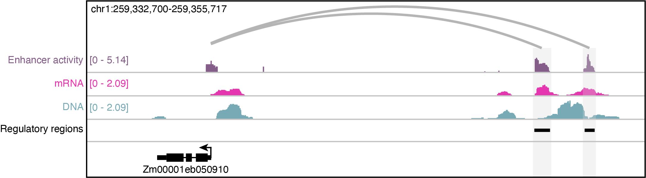
  Figure 3. Visualization of the assay for transposase accessible chromatin profiling followed by self-transcribed active regulatory region sequencing (ATAC-STARR-seq) data in Zea mays. Normalized (reads per million) coverages of the DNA ATAC-seq input (blue), self-transcribed mRNA fragments (pink), and enhancer activity [purple; log₂(mRNA/DNA)] of a 23 kb window. Regulatory regions are shown as black bars, while the grey loops reflect predicted enhancer-gene links.
Create a list of control regions
To assess enrichment of STARR regulatory regions determined by MACS2 relative to random control regions, we first need to identify regions of the genome that can be uniquely mapped given the sequencing output and read lengths. Although there are numerous methods for estimating mappability, I illustrate a simple approach using synthetic reads tailored to the sequencing parameters of the present experiment. First, we generate the same number of random read pairs with the same sequencing length (36 nucleotides) for mRNA and DNA input using the wgsim tool that is supplied to SAMtools. The synthetic reads are then remapped and uniformly processed as the original STARR-seq sequencing experiments to identify regions that are uniquely mappable. By constraining randomized control region selection to uniquely mappable genomic intervals, we ensure that downstream comparisons will not be biased by mappability and repeat composition. A script to construct control regions can be found here: https://github.com/Bio-protocol/Maize_ATAC_STARR_seq/blob/master/workflow/step06_create_control_regions.sh

# move into the “Genome_Reference” directory
cd ./Genome_Reference

# estimate read counts
mRNA_counts=$(samtools view -c ./BAM_files/B73_maize_mRNA_output.raw.bam)
DNA_counts=$(samtools view -c ./BAM_files/B73_maize_DNA_input.raw.bam)

# generate simulated reads matching the mRNA output using wgsim from the SAMtools package
wgsim -1 36 -2 36 -d 300 -N $mRNA_counts Zm-B73-REFERENCE-NAM-5.0.fa simulated_STARR_mRNA_r1.fq simualted_STARR_mRNA_r2.fq

# generate simulated reads matching the DNA input
wgsim -1 36 -2 36 -d 300 -N $DNA_counts Zm-B73-REFERENCE-NAM-5.0.fa simulated_STARR_DNA_r1.fq simualted_STARR_DNA_r2.fq

# compress synthetic fastq files
pigz *.fq
1. Remap the synthetic reads using the same pipeline as for the original STARR-seq data.
  
  # variables
  outdir=$PWD/BAM_files
  refdir=$PWD/Genome_Reference
  ref=$refdir/Zm-B73-REFERENCE-NAM-5.0.fa.fai.sorted
  fastqdir=$refdir
  
  # align synthetic mRNA output and pipe to samtools for SAM to BAM conversion
  bwa mem -M -t 24 $refdir/Zm-B73-REFERENCE-NAM-5.0.fa \
  $fastqdir/simulated_STARR_mRNA_r1.fq.gz \
  $fastqdir/simualted_STARR_mRNA_r2.fq.gz \
  | samtools view -bS - \
  | samtools sort - > $outdir/simulated_STARR_mRNA.raw.bam
  
  # align synthetic DNA input and pipe to samtools for SAM to BAM conversion
  bwa mem -M -t 24 $refdir/Zm-B73-REFERENCE-NAM-5.0.fa \
  $fastqdir/simulated_STARR_DNA_r1.fq.gz \
  $fastqdir/simulated_STARR_DNA_r2.fq.gz \
  | samtools view -bS - \
  | samtools sort - > $outdir/simulated_STARR_DNA.raw.bam
2. Process and filter reads using the original STARR-seq pipeline.
  
  # filter synthetic mRNA alignments
  echo " filtering synthetic STARR mRNA alignments ..."
  samtools view -h -q 10 -f 3 $outdir/simulated_STARR_mRNA.raw.bam \
  | grep -v -E -e '\bXA:Z:' \
  | samtools view -bSh - > $outdir/simulated_STARR_mRNA.mq10.pp.unique.bam
  
  # filter synthetic DNA alignments
  echo " filtering STARR DNA alignments ..."
  samtools view -h -q 10 -f 3 $outdir/simulated_STARR_DNA.raw.bam \
  | grep -v -E -e '\bXA:Z:' \
  | samtools view -bSh - > $outdir/simulated_STARR_DNA.mq10.pp.unique.bam
3. Identify uniquely mappable regions.
  
  # extract mRNA output fragments
  echo " extracting fragments from simulated STARR mRNA output ..."
  samtools sort -n $outdir/simulated_STARR_mRNA.mq10.pp.unique.bam \
  | bedtools bamtobed -bedpe -i - \
  | sort -k1,1 -k2,2n - \
  | cut -f1,2,6 - > $refdir/simulated_STARR_mRNA.fragments.bed
  
  # extract DNA input fragments
  echo " extracting fragments from simulated STARR DNA input ..."
  samtools sort -n $outdir/simulated_STARR_DNA.mq10.pp.unique.bam \
  | bedtools bamtobed -bedpe -i - \
  | sort -k1,1 -k2,2n - \
  | cut -f1,2,6 - > $refdir/simulated_STARR_DNA.fragments.bed
  
  # merge all fragments (sorting by coordinate at this step may take a while)
  cat $refdir/simulated_STARR_mRNA.fragments.bed $refdir/simulated_STARR_DNA.fragments.bed \
  | sort -k1,1 -k2,2n \
  | bedtools merge -i - > $refdir/mappable_genomic_regions.bed
4. Construct control regions using only mappable regions and excluding putative regulatory regions output by MACS2.
  
  # create controls
  peaks=$PWD/Peak_data/STARR_merged_peaks.bed
  bedtools shuffle -i $peaks \
  -g $ref \
  -incl $refdir/mappable_genomic_regions.bed \
  -excl $peaks \
  | sort -k1,1 -k2,2n - > $PWD/Peak_data/STARR_CONTROL.bed
Compare enhancer activity
1. Determine enhancer activity for predicted enhancers output by MACS2 as well as the negative control regions.
  
  # create directory to contain analysis
  cd ../
  mkdir 01_Peak_Analysis
  cd 01_Peak_Analysis
  
  # map maximum enhancer activity to putative regulatory regions (wdups)
  bedtools map -a ../Peak_data/STARR_merged_peaks.bed -b ../BED_files/B73_maize.enhancer_activity.bdg -o max -c 4 > STARR_merged_peaks.enhancer_activity.bed
  
  # map maximum enhancer activity to control
  bedtools map -a ../Peak_data/STARR_CONTROL.bed -b ../BED_files/B73_maize.enhancer_activity.bdg -o max -c 4 > STARR_CONTROL.enhancer_activity.bed
2. To remove regulatory regions with enhancer activity similar to background, we filter STARR regulatory regions using an empirical false discovery rate (eFDR) based on the matched control regions. A user-specified eFDR threshold identifies the enhancer activity value in the control set that removes 1-eFDR percent of control regions. In this example, we set the FDR to a widely used rate of 0.05. The following code performs and plots eFDR filtering and enhancer activity distributions and can be run from the command line using >Rscript eFDR_Filter_STARR_Peaks.R. Filtering STARR peaks based on eFDR thresholds derived from the control regions is visualized in Figure 4A. An R script of the following code can be found here: https://github.com/Bio-protocol/Maize_ATAC_STARR_seq/blob/master/workflow/bin/eFDR_Filter_STARR_Peaks.R
  
  # start an interactive R session
  > R
  
  # load libraries
  library(scales)
  
  # load data
  starr <- read.table("STARR_merged_peaks.enhancer_activity.bed")
  con <- read.table(”STARR_CONTROL.enhancer_activity.bed")
  
  # set missing to 0
  starr$V4[starr$V4=='.'] <- 0
  con$V4[con$V4=='.'] <- 0
  
  # convert to numeric
  starr$V4 <- as.numeric(as.character(starr$V4))
  con$V4 <- as.numeric(as.character(con$V4))
  
  # get empirical thresholds
  fdr <- 0.05
  threshold <- quantile(con$V4, (1-fdr))
  
  # filter STARR regulatory regions
  filtered <- subset(starr, starr$V4 >= threshold)
  
  # estimate fraction of retained regions
  frac <- signif(nrow(filtered)/nrow(starr), digits=4)
  
  # set up multipanel plot area
  pdf("Density_eFDR_STARR_Peak_Filtering.pdf", width=5, height=5)
  
  # plot control/observed enhancer activities for STARR peaks with duplicates
  den.starr <- density(starr$V4)
  den.con <- density(con$V4)
  plot(NA,
  xlab="Enhancer Activity",
  ylab="Density",
  xlim=c(range(range(den.starr$x), range(den.con $x))),
  ylim=c(range(range(den.starr$y), range(den.con$y))))
  polygon(x=c(min(den.starr$x), den.starr$x, max(den.starr$x)),
  y=c(0, den.starr$y, 0), col=alpha("darkorchid4", 0.5), border=NA)
  polygon(x=c(min(den.con$x), den.con$x, max(den.con$x)),
  y=c(0, den.con$y, 0), col=alpha("grey80", 0.5), border=NA)
  abline(v=threshold, col="red", lty=2)
  mtext(paste0("STARR peaks pass = ",frac," (", nrow(filtered), "/", nrow(starr),")"))
  
  legend("right", legend=c("STARR Peaks", "Control Peaks", paste0("eFDR = ", fdr)), col=c("darkorchid4", "grey75", "red"), border=c(NA, NA, "red"), pch=c(16, 16, NA), lty=c(NA, NA, 2))
  
  # close device
  dev.off()
  
  # save filtered STARR regulatory regions
  write.table(filtered, file="STARR_merged_peaks.enhancer_activity.eFDR05.bed", quote=F, row.names=F, col.names=F, sep="\t")
  
  # exit R
  q()
  
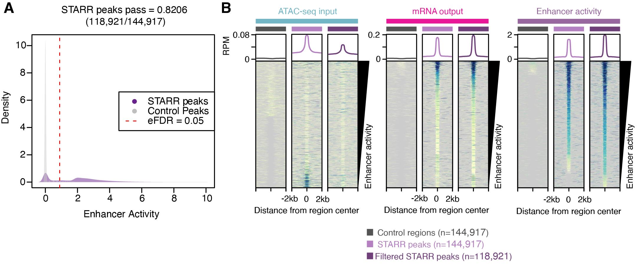
  Figure 4. Analysis of self-transcribed active regulatory region (STARR) regulatory region enhancer activity. A. Distribution of enhancer activity for STARR peaks (purple) and random control regions (grey). Dashed red line indicates the 95% quantile of enhancer activity of random control regions. B. Average (top) and individual site heatmaps of reads per million (RPM) for ATAC-seq input (left), mRNA output (middle), and enhancer activity (right) for control regions, all STARR peaks, and the filtered STARR peak set.
3. We can now assess the relative enhancer activities across all regions for the filtered and unfiltered STARR peaks and controls using DeepTools (Figure 4B). A script to plot heatmaps via DeepTools can be found here: https://github.com/Bio-protocol/Maize_ATAC_STARR_seq/blob/master/workflow/step07_plot_enhancer_activity.sh
  
  # load function
  getmaps(){
  
  # input
  ina=$1
  id=$2
  dat=../BED_files/*.bw
  
  # output
  outa=$id.mat.gz
  outm=$id.mat.txt
  fig=$id.pdf
  
  # parameters
  threads=48
  window=2000
  bin=20
  cols=YlGnBu
  
  # create matrix
  computeMatrix reference-point --referencePoint center \
  -S $dat \
  -b $window -a $window \
  -R $ina \
  --missingDataAsZero \
  -o $outa \
  --outFileNameMatrix $outm \
  -p $threads --binSize $bin
  
  # plot heatmap
  plotHeatmap --matrixFile $outa \
  --colorMap YlGnBu \
  -out $id.heatmap.pdf
  }
  export -f getmaps
  
  # run for each file
  getmaps STARR_merged_peaks.enhancer_activity.bed STARR_peaks
  getmaps STARR_merged_peaks.enhancer_activity.eFDR05.bed STARR_peaks_filtered
  getmaps STARR_CONTROL.enhancer_activity.bed control_regions
Identification of large regulatory domains in the maize genome
1. One question these data allow us to ask is whether a relationship exists between the size of a regulatory region and its enhancer activity. The so called super enhancers in mammalian systems describe hyperactive transcription-activating regulatory domains associated with cell identity that exhibit increased density of TF binding sites compared to typical enhancers (Hnisz et al., 2013). Integration of the STARR peaks and enhancer activities with other datasets allows us to determine whether similar hyperactive regulatory domains exist in maize. To query TF binding site density, we first download the position weight matrices of known TFs from the MEME database and identify putative TF binding sites using fimo (also from the MEME suite) conditioning on a P-value threshold less than 1^-5. A script to identify large regulatory domains can be found here: https://github.com/Bio-protocol/Maize_ATAC_STARR_seq/blob/master/workflow/step08_identify_large_regulatory_domains.sh
  
  # make a new directory for the TFBS analysis
  cd ../
  mkdir 02_Hyperactive_Regulatory_Region_Analysis
  cd ./02_Hyperactive_Regulatory_Region_Analysis
  
  # download and decompress motif databases
  wget https://meme-suite.org/meme/meme-software/Databases/motifs/motif_databases.12.23.tgz
  tar -xvzf motif_databases.12.23.tgz
  rm motif_databases.12.23.tgz
  
  # variables
  threads=16
  ref=../Genome_Reference/Zm-B73-REFERENCE-NAM-5.0.fa
  peaks=../01_Peak_Analysis/STARR_merged_peaks.enhancer_activity.eFDR05.bed
  controls=../01_Peak_Analysis/STARR_CONTROL.enhancer_activity.bed
  motifs=./motif_databases/ARABD/ArabidopsisDAPv1.meme
  
  # extract fasta sequences
  bedtools getfasta -bed $peaks -fi $ref -fo $peaks.fasta
  bedtools getfasta -bed $controls -fi $ref -fo $controls.fasta
  
  # identify putative TFBS
  fimo --oc TFBS_peaks $motifs $peaks.fasta
  fimo --oc TFBS_controls $motifs $controls.fasta
  
  # reformat fimo output (filtering p-value > 1e-5) using the perl script provided in the github repository (https://github.com/Bio-protocol/Maize_ATAC_STARR_seq/blob/master/workflow/bin/convertMotifCoord.pl )
  perl convertMotifCoord.pl TFBS_peaks/fimo.gff | sed -e 's/_tnt//g' - | sort -k1,1 -k2,2n - > TFBS_peaks.motifs.bed
  perl convertMotifCoord.pl TFBS_controls/fimo.gff | sed -e 's/_tnt//g' - | sort -k1,1 -k2,2n - > TFBS_controls.motifs.bed
  
  # annotate motif coverage/counts for STARR and control peaks
  bedtools annotate -i ../01_Peak_Analysis/STARR_merged_peaks.enhancer_activity.eFDR05.bed -files TFBS_peaks.motifs.bed -both | sort -k1,1 -k2,2n - > STARR_merged_peaks.enhancer_activity.eFDR05.ann.bed
  bedtools annotate -i ../01_Peak_Analysis/STARR_CONTROL.enhancer_activity.bed -files TFBS_controls.motifs.bed -both | sort -k1,1 -k2,2n - > STARR_CONTROL.enhancer_activity.ann.bed
  
  # extract genes
  perl -ne 'if($_ =~ /^#/){next;}chomp;my@col=split("\t",$_);if($col[2] eq 'gene'){print"$_\n";}' ../Genome_Reference/Zm-B73-REFERENCE-NAM-5.0_Zm00001eb.1.gff3 | sort -k1,1 -k4,4n - > ../Genome_Reference/Zm-B73-REFERENCE-NAM-5.0_Zm00001eb.1.genes.gff3
  
  # classify genomic context of STARR and control peaks (you can ignore the warnings from bedtools about inconsistent naming conventions, you can thank the genome assembly team for these annoying, but harmless warnings)
  bedtools closest -a STARR_merged_peaks.enhancer_activity.eFDR05.ann.bed -b ../Genome_Reference/Zm-B73-REFERENCE-NAM-5.0_Zm00001eb.1.genes.gff3 -D b > STARR_merged_peaks.enhancer_activity.eFDR05.ann2.bed
  bedtools closest -a STARR_CONTROL.enhancer_activity.ann.bed -b ../Genome_Reference/Zm-B73-REFERENCE-NAM-5.0_Zm00001eb.1.genes.gff3 -D b > STARR_CONTROL.enhancer_activity.ann2.bed
  
  # clean up
  mv STARR_merged_peaks.enhancer_activity.eFDR05.ann2.bed STARR_merged_peaks.enhancer_activity.eFDR05.ann.bed
  mv STARR_CONTROL.enhancer_activity.ann2.bed STARR_CONTROL.enhancer_activity.ann.bed
2. We can now investigate the relationship among regulatory region size, motif density, and enhancer activity to identify putative regulatory domains (Figure 5A–5F). To do so, we will start an interactive R session and load the annotated peak and control files from above. A script to automate the following code can be found here: https://github.com/Bio-protocol/Maize_ATAC_STARR_seq/blob/master/workflow/bin/Characterize_Regulatory_Regions.R
  
  # open R
  > R
  # Analyze regulatory regions
  
  # load libraries
  library(vioplot)
  library(dplyr)
  library(MASS)
  library(RColorBrewer)
  library(scales)
  
  # load data
  starr <- read.table("STARR_merged_peaks.enhancer_activity.eFDR05.ann.bed")
  control <- read.table("STARR_CONTROL.enhancer_activity.ann.bed")
  
  # select random control regions to match the filtered STARR peaks
  control <- control[sample(nrow(starr)),]
  
  # rename columns for clarity (frac_RR_motif = fraction of regulatory region covered by motifs)
  starr[,7:15] <- NULL
  control[,7:15] <- NULL
  colnames(starr)[4:7] <- c("activity", "motif_counts", "frac_RR_motif", "gene_distance")
  colnames(control)[4:7] <- c("activity", "motif_counts", "frac_RR_motif", "gene_distance")
  
  # classify
  starr$class <- ifelse((starr$gene_distance < 0 & starr$gene_distance > -200), "TSS", ifelse(starr$gene_distance < -200 & starr$gene_distance > -2000, "promoter", ifelse(starr$gene_distance > 0 & starr$gene_distance < 1000, "TTS", ifelse(starr$gene_distance == 0, "genic", "intergenic"))))
  
  control$class <- ifelse((control$gene_distance < 0 & control$gene_distance > -200), "TSS", ifelse(control$gene_distance < -200 & control$gene_distance > -2000, "promoter", ifelse(control$gene_distance > 0 & control$gene_distance < 1000, "TTS", ifelse(control$gene_distance == 0, "genic", "intergenic"))))
  
  # plot distribution
  pdf("STARR_peak_control_genomic_distribution.pdf", width=10, height=5)
  layout(matrix(c(1:2), nrow=1))
  pie(table(starr$class))
  pie(table(control$class))
  dev.off()
  
  # estimate regulatory region size (in log10 scale)
  starr$size <- log10(starr$V3-starr$V2)
  control$size <- log10(control$V3-control$V2)
  
  # compare sizes between peaks and controls (sanity check)
  pdf("STARR_peak_control_sizes.pdf", width=5, height=6)
  vioplot(starr$size, control$size,
  ylab="Interval size (log10)",
  col=c("dodgerblue", "grey75"),
  names=c(paste0("STARR peaks \n (n=",nrow(starr),")"),
  paste0("Control regions \n (n=",nrow(control),")")))
  dev.off()
  
  # compare motif counts
  pval <- wilcox.test(starr$motif_counts, control$motif_counts)$p.value
  pval <- ifelse(pval==0, 2.2e-16, pval)
  mean.peak <- mean(starr$motif_counts)
  mean.cont <- mean(control$motif_counts)
  
  # find 95% quantile for control motif count
  upper.threshold <- quantile(control$motif_counts, 0.95)
  
  # plot
  pdf("STARR_peak_control_motif_counts.pdf", width=5, height=6)
  vioplot(log1p(starr$motif_counts), log1p(control$motif_counts),
  ylab="log2(Motif counts + 1)",
  col=c("dodgerblue", "grey75"),
  names=c(paste0("STARR peaks \n (n=",nrow(starr),")"),
  paste0("Control regions \n (n=",nrow(control),")")),
  ylim=c(0,8),
  areaEqual=T,
  h=0.25)
  mtext(paste0("Wilcoxon Rank Sum P-value = ", signif(pval, digits=3)))
  text(1, 7.5, labels=paste0("Mean = ", signif(mean.peak, digits=3)))
  text(2, 7.5, labels=paste0("Mean = ", signif(mean.cont, digits=3)))
  points(1, log1p(upper.threshold), col="red", pch="-")
  points(2, log1p(upper.threshold), col="red", pch="-")
  dev.off()
  
  # split STARR regions by motif counts based on 95% quantile control dist
  starr$group <- ifelse(starr$motif_counts >= upper.threshold, "high", "low")
  pval <- kruskal.test(starr$activity, starr$group)$p.value
  pdf("STARR_peak_activity_vs_group.pdf", width=5, height=6)
  vioplot(starr$activity~starr$group,
  ylab="Enhancer activity",
  col=c("dodgerblue4", "dodgerblue"),
  names=c(paste0("Motif-enriched \n STARR peaks \n (n=", nrow(starr[starr$group=="high",]),")"),
  paste0("Motif-depleted \n STARR peaks \n (n=", nrow(starr[starr$group=="low",]),")")),
  areaEqual=F,
  xlab="",
  h=0.25)
  mtext(paste0("Kruskal-Wallis rank sum P-value = ", signif(pval, digits=3)))
  dev.off()
  
  # compare STARR region size
  pval <- kruskal.test(starr$size, starr$group)$p.value
  pval <- ifelse(pval==0, 2.2e-16, pval)
  pdf("STARR_peak_size_vs_group.pdf", width=5, height=6)
  vioplot(starr$size~starr$group,
  ylab="Interval size (log10)",
  col=c("dodgerblue4", "dodgerblue"),
  names=c(paste0("Motif-enriched \n STARR peaks \n (n=", nrow(starr[starr$group=="high",]),")"),
  paste0("Motif-depleted \n STARR peaks \n (n=", nrow(starr[starr$group=="low",]),")")),
  areaEqual=F,
  xlab="",
  h=0.25)
  mtext(paste0("Kruskal-Wallis rank sum P-value = ", signif(pval, digits=3)))
  dev.off()
  
  # compare motif coverage
  pval <- kruskal.test(starr$frac_RR_motif, starr$group)$p.value
  pval <- ifelse(pval==0, 2.2e-16, pval)
  pdf("STARR_peak_motif_coverage_vs_group.pdf", width=5, height=6)
  vioplot(starr$frac_RR_motif~starr$group,
  ylab="Fraction motif coverage",
  col=c("dodgerblue4", "dodgerblue"),
  names=c(paste0("Motif-enriched \n STARR peaks \n (n=", nrow(starr[starr$group=="high",]),")"),
  paste0("Motif-depleted \n STARR peaks \n (n=", nrow(starr[starr$group=="low",]),")")),
  areaEqual=F,
  xlab="")
  mtext(paste0("Kruskal-Wallis rank sum P-value = ", signif(pval, digits=3)))
  dev.off()
  
  # split by group
  starr.me <- subset(starr, starr$group=="high")
  starr.md <- subset(starr, starr$group=="low")
  write.table(starr.me, file="STARR_starrs_peaks.enhancer_activity.eFDR05.ann.high_motif.bed",
  quote=F, row.names=F, col.names=F, sep="\t")
  write.table(starr.md, file="STARR_starrs_peaks.enhancer_activity.eFDR05.ann.low_motif.bed",
  quote=F, row.names=F, col.names=F, sep="\t")
  
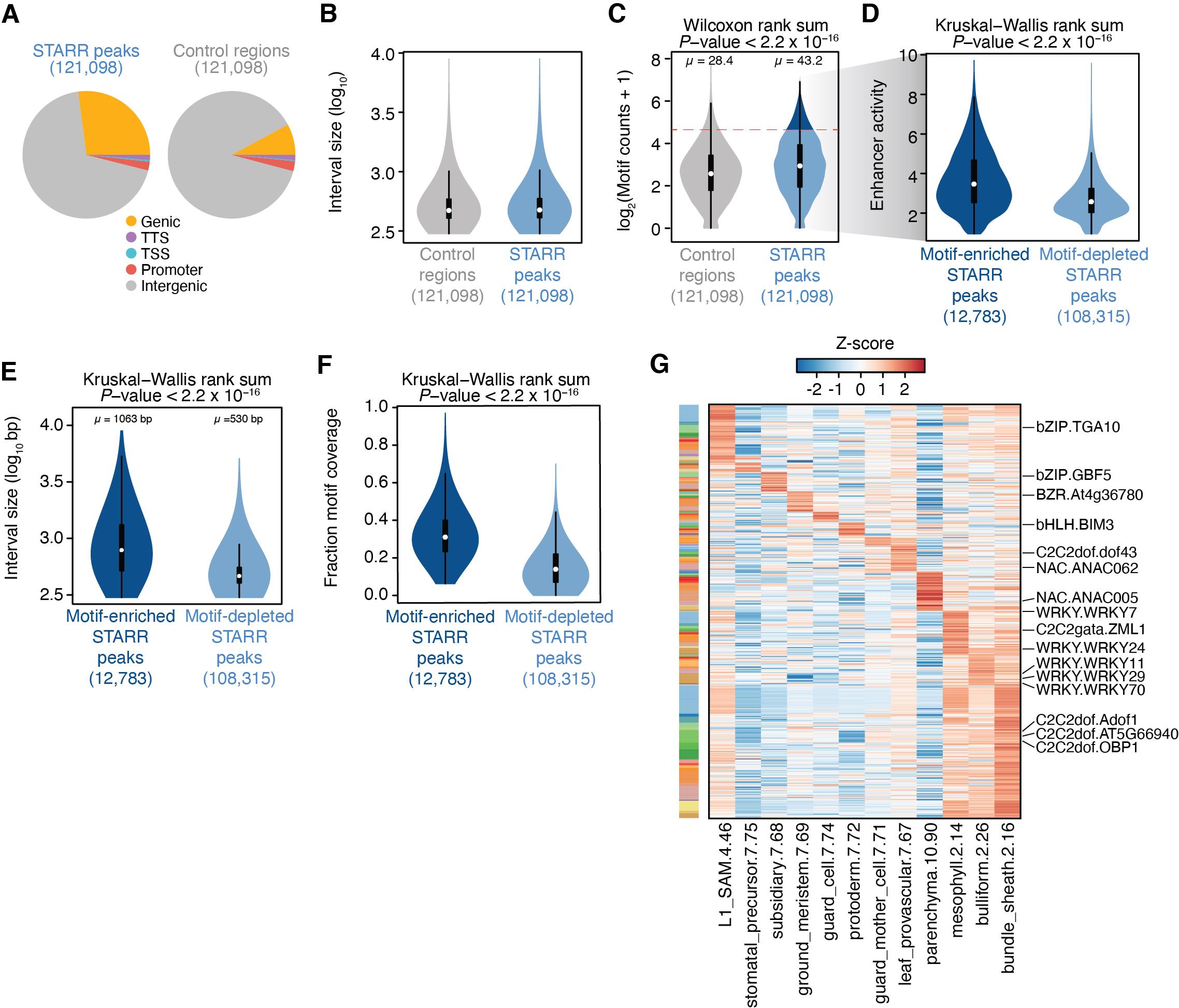
  Figure 5. Identification of motif-dense enhancer regulatory domains. A. Genomic distribution of self-transcribed active regulatory region (STARR) peaks (left) and control regions (right). B. Distribution of control region (grey) and STARR peak (blue) interval lengths. C. Distribution of motif counts in control regions (grey) and STARR peaks (blue). The dashed red line indicates the 95% quantile of motif counts from control regions used to classify STARR peaks into high- and low-motif count classes. D. Distribution of enhancer activity for STARR peaks with enriched (dark blue) and depleted (light blue) motif counts. E. Distribution of interval lengths for motif-enriched (dark blue) and motif-depleted (light blue) STARR peaks. F. Distribution of fraction of STARR peaks covered by motif for motif-enriched (dark blue) and motif-depleted (light blue) STARR peaks. G. Heatmap illustrating Z-score-transformed motif-enhancer activities across intergenic motif-enriched STARR peaks scaled by the relative chromatin accessibility in various maize cell types.
  
  3. To determine if the large intergenic regulatory domain regions are associated with cell identity, we will compare enhancer activities vs. various cell type–specific ACRs leveraging a recent single-cell ATAC-seq (scATAC-seq) dataset from multiple maize organs (Marand et al., 2021). First, download the matrix containing normalized accessibility counts across accessible chromatin regions for each profiled cell type. We then extract ACR genomic coordinates (which are in version 4 of the B73 reference genome) and convert them to version 5 of the B73 reference genome using the CrossMap tool and chain file.
  
  # download the counts matrix
  wget -O maize_scATAC_atlas_ACR_celltype_CPM.txt.gz https://www.ncbi.nlm.nih.gov/geo/download/\?acc\=GSE155178\&format\=file\&file\=GSE155178%5Fmaize%5FscATAC%5Fatlas%5FACR%5Fcelltype%5FCPM%2Etxt%2Egz
  
  # unzip
  gunzip maize_scATAC_atlas_ACR_celltype_CPM.txt.gz
  
  # download chain file
  wget https://download.maizegdb.org/Zm-B73-REFERENCE-NAM-5.0/chain_files/B73_RefGen_v4_to_Zm-B73-REFERENCE-NAM-5.0.chain
  
  # extract coordinates and conform chromosome names to V4 reference
  cut -f1 maize_scATAC_atlas_ACR_celltype_CPM.txt \
  | grep '^chr' - \
  | perl -ne 'chomp;my@col=split("_",$_);print"$col[0]\t$col[1]\t$col[2]\n";' - \
  | sed -e 's/chrB73V4ctg/B73V4_ctg/g' - \
  | sed -e 's/chr//g' - \
  | sort -k1,1 -k2,2n - > maize_scATAC_atlas_ACRs.bed
  
  # convert ACR coordinates from V4 to V5
  CrossMap.py bed B73_RefGen_v4_to_Zm-B73-REFERENCE-NAM-5.0.chain maize_scATAC_atlas_ACRs.bed > maize_scATAC_atlas_ACRs.V4_to_V5.txt
  
  # discard unmapped and split projections
  grep -v 'Unmap\|split' maize_scATAC_atlas_ACRs.V4_to_V5.txt \
  | perl -ne 'chomp; my@col=split("\t",$_); print"chr$col[0]_$col[1]_$col[2]\tchr$col[4]_$col[5]_$col[6]\n";' - \
  | sort -k1,1 -k2,2n - \
  | sed -e 's/chrscaf/scaf/g' - \
  | sed -e 's/chrB73V4_ctg/chrB73V4ctg/g' - > maize_scATAC_atlas_ACRs.V4_to_V5.clean.txt
  
  # update ACR coordinates in matrix file using R
  > R
  
  # read into data frames
  conv <- read.table("maize_scATAC_atlas_ACRs.V4_to_V5.clean.txt")
  mat <- read.table("maize_scATAC_atlas_ACR_celltype_CPM.txt")
  
  # subset mat rows by retained ACRs after projection
  shared <- intersect(rownames(mat), as.character(conv$V1))
  mat <- mat[shared,]
  rownames(conv) <- conv$V1
  conv <- conv[shared,]
  
  # update mat rowIDs
  rownames(mat) <- conv$V2
  
  # save output
  write.table(mat, file="maize_scATAC_atlas_ACR_celltype_CPM.V5.txt", quote=F, row.names=T, col.names=T, sep="\t")
  
  # exit R
  q()
  
  # remove temporary files
  rm maize_scATAC_atlas_ACR_celltype_CPM.txt maize_scATAC_atlas_ACRs.bed maize_scATAC_atlas_ACRs.V4_to_V5.txt maize_scATAC_atlas_ACRs.V4_to_V5.clean.txt
  
  4. Intersect the scATAC-seq ACRs with the STARR peaks with enriched motif counts. Load the scATAC-seq matrix and intersected ACRs/STARR peaks files into R to estimate enhancer activity enrichment scaled by relative accessibilities across cell types. As the STARR-seq data was derived from maize seedlings, we further restrict the analysis of scATAC-seq cell types to those derived primarily from maize seedlings. The following code written in R can be executed with the script named “motif_enhancer_activity_maize_celltypes.R” and provides estimates of enhancer activity over various motifs scaled by the relative cell type accessibility, allowing insights into cell type–specific transcription factor regulation of active enhancers (Figure 5G).
  
  # extract ACR coordinates
  cut -f1 maize_scATAC_atlas_ACR_celltype_CPM.V5.txt| grep -v 'unknown.5.50' | sed -e 's/scaf_/scaf/g' | perl -ne 'chomp;my@col=split("_",$_);print"$col[0]\t$col[1]\t$col[2]\n";' - | sed -e 's/scaf/scaf_/g' - | sort -k1,1 -k2,2n - > maize_scATAC_atlas_ACRs.V5.bed
  
  # intersect scATAC ACRs with high motif counts STARR peaks
  bedtools intersect -a STARR_starrs_peaks.enhancer_activity.eFDR05.ann.high_motif.bed -b maize_scATAC_atlas_ACRs.V5.bed -wa -wb > STARR_starrs_peaks.enhancer_activity.eFDR05.ann.high_motif.scATAC_ACRs.bed
  
  # map enhancer activity over motifs
  bedtools map -a TFBS_peaks.motifs.bed -b ../BED_files/B73_maize.enhancer_activity.bdg -c 4 -o max > TFBS_peaks.motifs.enhancer_activity.bed
  
  # motifs to large regulatory regions
  bedtools intersect -a TFBS_peaks.motifs.enhancer_activity.bed -b STARR_starrs_peaks.enhancer_activity.eFDR05.ann.high_motif.scATAC_ACRs.bed -wa -wb > TFBS_peaks.motifs.enhancer_activity.bed
  
  # open R (alternatively, a script to automate the following code can be found here: https://github.com/Bio-protocol/Maize_ATAC_STARR_seq/blob/master/workflow/bin/motif_enhancer_activity_maize_celltypes.R)
  > R
  
  # estimate enhancer activity cell type specificity
  
  # load libraries
  library(RColorBrewer)
  library(gplots)
  library(edgeR)
  
  # load data
  enh <- read.table("STARR_starrs_peaks.enhancer_activity.eFDR05.ann.high_motif.scATAC_ACRs.bed")
  acrs <- read.table("maize_scATAC_atlas_ACR_celltype_CPM.V5.txt")
  motifs <- read.table("TFBS_peaks.motifs.ENRICHED.enhancer_activity.bed")
  
  # subset for representative leaf-derived clusters
  keep <- c("bulliform.2.26",
  "bundle_sheath.2.16",
  "ground_meristem.7.69",
  "guard_cell.7.74",
  "guard_mother_cell.7.71",
  "L1_SAM.4.46",
  "leaf_provascular.7.67",
  "mesophyll.2.14",
  "parenchyma.10.90",
  "protoderm.7.72",
  "stomatal_precursor.7.75",
  "subsidiary.7.68")
  all.acrs <- acrs
  
  # rescale acrs
  acrs <- cpm(acrs, log=F)
  acrs <- acrs[,keep]
  
  # subset enhancers by genomic feature
  enh <- subset(enh, enh$V8=="intergenic")
  
  # get overlapping regions from the scATAC matrix
  enh$ids <- paste(enh$V11,enh$V12,enh$V13,sep="_")
  enh <- enh[order(enh$V11, decreasing=T),]
  enh <- enh[!duplicated(enh$ids),]
  shared <- intersect(enh$ids, rownames(acrs))
  rownames(enh) <- enh$ids
  enh <- enh[shared,]
  enh$starrIDs <- paste(enh$V1, enh$V2, enh$V3,sep="_")
  
  # filter motifs
  motifs$starrIDs <- paste(motifs$V5, motifs$V6, motifs$V7, sep="_")
  motifs <- motifs[motifs$starrIDs %in% unique(enh$starrIDs),]
  
  # normalize acrs
  acrs <- t(apply(acrs, 1, function(x){x/max(x)}))
  
  # iterate over each cell type
  cts <- colnames(acrs)
  outs <- lapply(cts, function(x){
  access <- acrs[rownames(enh),x]
  names(access) <- enh$starrIDs
  motif.scores <- access[motifs$starrIDs] * as.numeric(as.character(motifs$V15))
  mtf <- data.frame(motif=motifs$V4, score=motif.scores)
  aves <- aggregate(score~motif, data=mtf, FUN=mean)
  score <- aves$score
  names(score) <- aves$motif
  return(score)
  })
  outs <- do.call(cbind, outs)
  colnames(outs) <- cts
  vars <- apply(outs, 1, var)
  outs <- outs[vars > 0,]
  z <- as.matrix(t(scale(t(outs))))
  
  # # cluster columns
  co <- hclust(dist(t(outs)))$order
  
  # reorder rows
  z <- z[,co]
  row.o <- apply(z, 1, which.max)
  z <- z[order(row.o, decreasing=F),]
  
  # cap
  z[z < -3] <- -3
  z[z > 3] <- 3
  
  # get family
  tfs <- data.frame(do.call(rbind, strsplit(rownames(z), "\\.")))
  cols2 <- colorRampPalette(brewer.pal(12, "Paired"))(length(unique(tfs$X1)))
  tfs$cols2 <- cols2[factor(tfs$X1)]
  
  # visualize
  pdf("celltype_starr_motif_activity.pdf", width=10, height=10)
  heatmap.2(z, scale="none", trace='none',
  RowSideColors=tfs$cols,
  col=colorRampPalette(rev(brewer.pal(9, "RdBu")))(100),
  useRaster=T, Colv=F, Rowv=F, dendrogram="none", margins=c(9,9))
  dev.off()

Acknowledgments

This study was funded by support from the National Science Foundation (DBI-1906869) and the National Institute of Health (1K99GM144742) to A.P.M. The ATAC-STARR-seq data analyzed in this study was originally generated by Ricci, Lu, Ji, and colleagues (Ricci et al., 2019).

Competing interests

A.P.M. declares no competing interests.

References

Arnold, C. D., Gerlach, D., Stelzer, C., Boryn, L. M., Rath, M. and Stark, A. (2013). Genome-wide quantitative enhancer activity maps identified by STARR-seq. Science 339(6123): 1074-1077.
Buenrostro, J. D., Giresi, P. G., Zaba, L. C., Chang, H. Y. and Greenleaf, W. J. (2013). Transposition of native chromatin for fast and sensitive epigenomic profiling of open chromatin, DNA-binding proteins and nucleosome position. Nat Methods 10(12): 1213-1218.
Chen, S., Zhou, Y., Chen, Y. and Gu, J. (2018). fastp: an ultra-fast all-in-one FASTQ preprocessor. Bioinformatics 34(17): i884-i890.
Grant, C. E., Bailey, T. L. and Noble, W. S. (2011). FIMO: scanning for occurrences of a given motif. Bioinformatics 27(7): 1017-1018.
Hnisz, D., Abraham, B. J., Lee, T. I., Lau, A., Saint-Andre, V., Sigova, A. A., Hoke, H. A. and Young, R. A. (2013). Super-enhancers in the control of cell identity and disease. Cell 155(4): 934-947.
Hufford, M. B., Seetharam, A. S., Woodhouse, M. R., Chougule, K. M., Ou, S., Liu, J., Ricci, W. A., Guo, T., Olson, A., Qiu, Y., et al. (2021). De novo assembly, annotation, and comparative analysis of 26 diverse maize genomes. Science 373(6555): 655-662.
Jores, T., Tonnies, J., Dorrity, M. W., Cuperus, J. T., Fields, S. and Queitsch, C. (2020). Identification of Plant Enhancers and Their Constituent Elements by STARR-seq in Tobacco Leaves^[OPEN]. The Plant Cell 32(7): 2120-2131.
Kent, W. J., Zweig, A. S., Barber, G., Hinrichs, A. S. and Karolchik, D. (2010). BigWig and BigBed: enabling browsing of large distributed datasets. Bioinformatics 26(17): 2204-2207.
Leinonen, R., Sugawara, H., Shumway, M. and International Nucleotide Sequence Database, C. (2011). The sequence read archive. Nucleic Acids Res 39(Database issue): D19-21.
Li, H. (2011). Tabix: fast retrieval of sequence features from generic TAB-delimited files. Bioinformatics 27(5): 718-719.
Li, H. and Durbin, R. (2009). Fast and accurate short read alignment with Burrows-Wheeler transform. Bioinformatics 25(14): 1754-1760.
Li, H., Handsaker, B., Wysoker, A., Fennell, T., Ruan, J., Homer, N., Marth, G., Abecasis, G., Durbin, R. and Genome Project Data Processing, S. (2009). The Sequence Alignment/Map format and SAMtools. Bioinformatics 25(16): 2078-2079.
Liu, T. (2014). Use model-based Analysis of ChIP-Seq (MACS) to analyze short reads generated by sequencing protein-DNA interactions in embryonic stem cells. Methods Mol Biol 1150: 81-95.
Marand, A. P., Chen, Z., Gallavotti, A. and Schmitz, R. J. (2021). A cis-regulatory atlas in maize at single-cell resolution. Cell 184(11): 3041-3055. e21.
Marand, A. P., Zhang, T., Zhu, B. and Jiang, J. (2017). Towards genome-wide prediction and characterization of enhancers in plants. Biochim Biophys Acta Gene Regul Mech 1860(1): 131-139.
Melnikov, A., Murugan, A., Zhang, X., Tesileanu, T., Wang, L., Rogov, P., Feizi, S., Gnirke, A., Callan, C. G., Kinney, J. B., et al. (2012). Systematic dissection and optimization of inducible enhancers in human cells using a massively parallel reporter assay. Nature Biotechnology 30(3): 271-277.
Minnoye, L., Marinov, G. K., Krausgruber, T., Pan, L., Marand, A. P., Secchia, S., Greenleaf, W. J., Furlong, E. E. M., Zhao, K., Schmitz, R. J., et al. (2021). Chromatin accessibility profiling methods. Nature Reviews Methods Primers 1(1): 10.
Quinlan, A. R. and Hall, I. M. (2010). BEDTools: a flexible suite of utilities for comparing genomic features. Bioinformatics 26(6): 841-842.
Ramirez, F., Dundar, F., Diehl, S., Gruning, B. A. and Manke, T. (2014). deepTools: a flexible platform for exploring deep-sequencing data. Nucleic Acids Res 42(Web Server issue): W187-191.
Ricci, W. A., Lu, Z., Ji, L., Marand, A. P., Ethridge, C. L., Murphy, N. G., Noshay, J. M., Galli, M., Mejia-Guerra, M. K., Colome-Tatche, M., et al. (2019). Widespread long-range cis-regulatory elements in the maize genome. Nat Plants 5(12): 1237-1249.
Schmitz, R. J., Grotewold, E. and Stam, M. (2022). Cis-regulatory sequences in plants: Their importance, discovery, and future challenges. Plant Cell 34(2): 718-741.
Sun, J., He, N., Niu, L., Huang, Y., Shen, W., Zhang, Y., Li, L. and Hou, C. (2019). Global Quantitative Mapping of Enhancers in Rice by STARR-seq. Genomics Proteomics Bioinformatics 17(2): 140-153.
Thorvaldsdottir, H., Robinson, J. T. and Mesirov, J. P. (2013). Integrative Genomics Viewer (IGV): high-performance genomics data visualization and exploration. Brief Bioinform 14(2): 178-192.
Zhao, H., Sun, Z. F., Wang, J., Huang, H. J., Kocher, J. P. and Wang, L. G. (2014). CrossMap: a versatile tool for coordinate conversion between genome assemblies. Bioinformatics 30(7): 1006-1007.

Supplementary information

Data and code availability: All data and code have been deposited to GitHub: https://github.com/Bio-protocol/Maize_ATAC_STARR_seq

Article Information

Copyright

How to cite

Marand, A. P. (2024). Computational Analysis of Maize Enhancer Regulatory Elements Using ATAC-STARR-seq. Bio-101: e4953. DOI: 10.21769/BioProtoc.4953.

Download Citation in RIS Format