- Protocols

- Articles and Issues
- For Authors
- About
- Become a Reviewer

Resolving the In Situ Three-Dimensional Structure of Fly Mechanosensory Organelles Using Serial Section Electron Tomography
(*contributed equally to this work) Published: Vol 14, Iss 4, Feb 20, 2024 DOI: 10.21769/BioProtoc.4940 Views: 3162
Reviewed by: Xiaokang WuRama Reddy GoluguriChen Fan
Original research article
The authors used this protocol in:

Aug 2023
Advertisement


Protocol Collections
Comprehensive collections of detailed, peer-reviewed protocols focusing on specific topics


Abstract
Mechanosensory organelles (MOs) are specialized subcellular entities where force-sensitive channels and supporting structures (e.g., microtubule cytoskeleton) are organized in an orderly manner. The delicate structure of MOs needs to be resolved to understand the mechanisms by which they detect forces and how they are formed. Here, we describe a protocol that allows obtaining detailed information about the nanoscopic ultrastructure of fly MOs by using serial section electron tomography (SS-ET). To preserve fine structural details, the tissues are cryo-immobilized using a high-pressure freezer followed by freeze-substitution at low temperature and embedding in resin at room temperature. Then, sample sections are prepared and used to acquire the dual-axis tilt series images, which are further processed for tomographic reconstruction. Finally, tomograms of consecutive sections are combined into a single larger volume using microtubules as fiducial markers. Using this protocol, we managed to reconstruct the sensory organelles, which provide novel molecular insights as to how fly mechanosensory organelles work and are formed. Based on our experience, we think that, with minimal modifications, this protocol can be adapted to a wide range of applications using different cell and tissue samples.
Key features
• Resolving the high-resolution 3D ultrastructure of subcellular organelles using serial section electron tomography (SS-ET).
• Compared with single-axis tilt series, dual-axis tilt series provides a much wider coverage of Fourier space, improving resolution and features in the reconstructed tomograms.
• The use of high-pressure freezing and freeze-substitution maximally preserves the fine structural details.
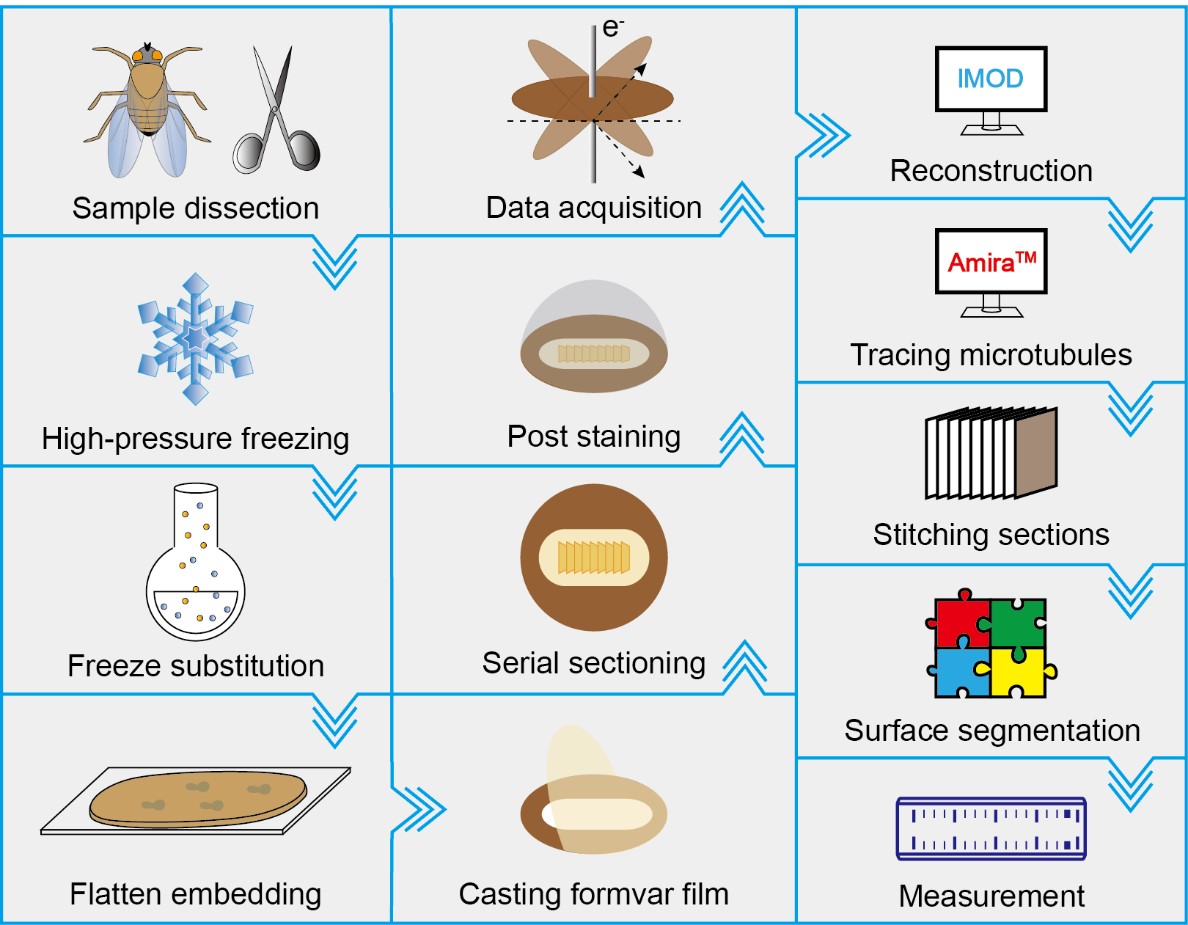
Graphical overview
Background
Drosophila type I sensory cells serve as a model for the study of mechanosensation, neuronal cell biology, and ciliogenesis due to their compatibility with functional, imaging, and structural assays [1–3]. In particular, the convenience of performing ultrastructural analysis has facilitated mechanistic studies on the above-mentioned topics, especially for understanding the molecular mechanisms of neurosensory transduction.
Mechanotransduction is the process by which mechanoreceptor cells convert physical signals in the environment into cellular signals [1,2,4]. Mechanoreceptors form a specialized functional entity called mechanosensory organelles (MOs) [5–11]. Because MOs are essentially mechanosensors, they possess a dedicated structural architecture that facilitates the detection of mechanical stimuli. To suit this purpose, MOs develop a delicate intracellular structure [5,7,8,11]. Information regarding this structure is required to understand how mechanosensory cells encode mechanical signals and are formed.
We and others have previously studied the ultrastructure of fly external mechanosensory cells using conventional transmission electron microscopy (TEM)[8,9,12–15]. These studies made a clear presentation of nanoscopic ultrastructures and provided molecular insights. However, the 3D structure of mechanosensory organelles and organization of the sensory molecules are absent. This information allows molecular interpretation of how the force-sensitive molecules transduce mechanical signals and how the specialized structures are formed. To solve these issues, we recently established a protocol for serial section electron tomography (SS-ET) [11,16,17]. Using this protocol, we successfully resolved the delicate structure and molecular organization of the MOs. Together with cell biological and modeling analysis, the structural analysis has been useful in understanding the working mechanism of fly MOs and how they are formed.
Electron tomography (ET) acquires a series of 2D projection images, known as tilt series, by incrementally varying the orientation of the sample relative to the incident electron beam. Using computational methods, the set of 2D images can be processed to yield a tomographic volume reconstruction at nanometer resolution [18,19]. However, the imaging depth of ET is restricted to a few hundred nanometers due to the limited penetration depth of electrons. Therefore, it is recommended that the thickness of plastic samples should be less than 300 nm for the most widely used TEMs. SS-ET, which merges the tomographic volume constructions from consecutive sections, compensates for this limitation to some extent [20,21].
Materials and reagents
Biological materials
Drosophila flies, maintained on a standard medium at 23 to 25 °C
Reagents
Carbon dioxide (CO2) (any supplier)
Sodium dihydrogen phosphate dihydrate (NaH2PO4 ·2H2O) (analytical grade) (e.g., Sinopharm Chemical Reagent Co., Ltd., catalog number: 20040718)
Disodium hydrogen phosphate dodecahydrate (Na2HPO4 ·12H2O) (analytical grade) (e.g., Sinopharm Chemical Reagent Co., Ltd., catalog number: 10020318)
Albumin bovine serum (BSA) (Sigma-Aldrich, catalog number: A9647)
Liquid nitrogen (any supplier)
Osmium tetroxide (Electron Microscopy Sciences, catalog number: 19110)
Glutaraldehyde (25% aqueous solution) (Electron Microscopy Sciences, catalog number: 16220)
Uranyl acetate (Polysciences, catalog number: 21447 or Electron Microscopy Sciences, catalog number: 22400)
Lead citrate (Electron Microscopy Sciences, catalog number: 17800)
Anhydrous acetone (analytical grade) (e.g., Electron Microscopy Sciences, catalog number: 10015)
Sodium hydroxide (NaOH) (Sigma-Aldrich, catalog number: 221465)
Araldite/embed-812 embedding kit (Electron Microscopy Sciences, catalog number: 13940), including embed-812, araldite, DDSA, and DMP-30
Teflon (Miller-Stephenson Chemical Co., Inc., U.S.A.)
Cyanoacrylic adhesive (any supplier)
Chloroform (analytical grade) (e.g., Electron Microscopy Sciences, catalog number: 12540)
Formvar 15/95 resin (Electron Microscopy Sciences, catalog number: 15800)
Methanol (analytical grade) (e.g., RHAWN, catalog number: R007542-4L)
Gold colloid (BBI Solutions, catalog number: EM. GC15)
Solutions
Phosphate buffer (0.1 mol/L, pH 7.2) (see Recipes)
20% BSA solution (see Recipes)
10% osmium tetroxide (see Recipes)
20% uranyl acetate (see Recipes)
Freeze-substitution solution (see Recipes)
30%, 50%, 70% aqueous methanol (see Recipes)
2% uranyl acetate (see Recipes)
10 mol/L NaOH (see Recipes)
0.4% lead citrate (see Recipes)
Araldite/embed-812 embedding media (see Recipes)
1%–3% formvar casting solution (see Recipes)
Recipes
Phosphate buffer (0.1 mol/L, pH 7.2)
Reagent Final concentration Quantity or volume NaH2PO 4·2H2O 0.437% (w/v) 0.437 g Na2HPO4·12H2O 2.579% (w/v) 2.579 g Ultrapure water n/a 100.0 mL Total n/a 100.0 mL 20% BSA (wt/vol) solution
Reagent Final concentration Quantity or volume BSA 20% (w/v) 0.2 g Phosphate buffer (0.1 mol/L, pH 7.2) n/a 0.8 mL Total n/a 1.0 mL 10% osmium tetroxide
Reagent Final concentration Quantity or volume Osmium tetroxide 10% (w/v) 1.0 mg Anhydrous acetone n/a 10 mL Total n/a 10 mL Caution: Osmium tetroxide is highly toxic and fatal. Handle it in a fume hood and wear personal protective equipment.
20% uranyl acetate
Reagent Final concentration Quantity or volume Uranyl acetate 20% (w/v) 0.2 mg Anhydrous methanol n/a 1.0 mL Total n/a 1.0 mL Caution: Uranyl acetate is toxic and slightly radioactive. Handle it in a fume hood and wear personal protective equipment.
Freeze-substitution solution
Reagent Final concentration Quantity or volume 10% osmium tetroxide 1% (w/v) 1.0 mL 20% uranyl acetate 0.1% (w/v) 50 μL 25% aqueous glutaraldehyde 0.5% (w/v) 200 μL Ultrapure water 4% (v/v) 250 μL Anhydrous acetone n/a 8.5 mL Total n/a 10 mL Caution: Freeze-substitution solution contains toxic and radioactive compounds. Handle them inside a fume hood and wear personal protective equipment.
30%, 50%, 70% aqueous methanol
Add 30, 50, and 70 mL of anhydrous methanol into 70, 50, and 30 mL of ultrapure water, respectively. Then, mix each aqueous methanol thoroughly by vortexing. Leave them at room temperature overnight or shake them in an ultrasonic cleaner for ~10 min to remove all air bubbles inside the aqueous methanol.
2% uranyl acetate
Note: Filter the solution using a 0.22 μm syringe filter unit or centrifuge the solution at 10,625× g for 10 min and then collect the filtrate or supernatant to use.
Reagent Final concentration Quantity or volume Uranyl acetate 2% (w/v) 0.2 g 70% aqueous methanol n/a 10 mL Total n/a 10 mL 10 mol/L NaOH
Note: Boil the ultrapure water for 15–30 min and then cool it to room temperature before use.
Reagent Final concentration Quantity or volume NaOH 10 mol/L 4.2 g Cooled boiled water n/a 10 mL Total n/a 10 mL 0.4% lead citrate
Note: Add 0.2 g of lead citrate into 50 mL of cooled boiled water in a 50 mL centrifuge tube. Immediately turn the tubes upside down several times and add 500 μL of 10 mol/L NaOH in it. Shake the tubes on an orbital shaker for at least 30 min and place them in the fume hood for at least two days before use.
Reagent Final concentration Quantity or volume Lead citrate 0.4% (w/v) 0.2 g 10 mol/L NaOH n/a 500 μL Cooled boiled water n/a 50 mL Total n/a 50 mL Araldite/embed-812 embedding media
Reagent Final concentration Quantity or volume Embed-812 n/a 62.0 g Araldite 502 n/a 44.4 g DDSA n/a 122.0 g DMP-30 n/a 5.5 mL Total n/a n/a Caution: Unpolymerized embedding media are toxic. Handle them in a fume hood and wear personal protective equipment.
1%–3% formvar casting solution
Reagent Final concentration Quantity or volume Formvar 15/95 resin 1%–3% (w/v) 1–3 g Chloroform n/a 100 mL Total n/a 100 mL
Laboratory supplies
Microcentrifuge tubes (0.2, 0.5, 1.5, and 2.0 mL) (e.g., Eppendorf, catalog number: 0030124332, 0030121023, 0030120086, and 0030120094, respectively)
Centrifuge tubes (15 and 50 mL) (e.g., Corning, catalog number: 430052 and 430290, respectively)
Petri dishes (30 and 100 mm) (e.g., Corning, catalog number: CLS430165 and CLS430167, respectively)
2 mL screwcap microtubes (Sarstedt AG & Co. KG, catalog number: 72.694.005)
0.22 μm syringe filter unit (Merck Millipore Ltd. catalog number: SLGPR33RS)
Aluminum foil (any supplier)
Pipette tips (0.1–20, 2–200, and 50–1,000 μL) (e.g., Eppendorf, catalog number: 0030000838, 0030000870, and 0030000919, respectively)
Cellulose capillary tubes (Leica Microsystems, catalog number: 16706869)
100 μm deep membrane carriers (Leica Microsystems, catalog number: 16707898)
Stainless steel surgical blades #23 (any supplier)
Surgical blade handles #3 (any supplier)
Plastic beakers (any supplier)
Plastic droppers (any supplier)
Amber glass bottles (any supplier)
Parafilm (Bemis, catalog number: PM996)
Fine tip needle (any supplier)
Glass slides (any supplier)
Slide storage boxes (any supplier)
Single-edge razor blades (any supplier)
Double-edge razor blades (any supplier)
Copper slot grids (Gilder Grids, catalog number: GS2X1-C3)
Filter papers (any supplier)
Cylindrical funnel (any supplier)
ACLAR® 33C film (Electron Microscopy Sciences, catalog number: 50425-10)
Kimwipes tissue (Kimberly-Clark, catalog number: 34155)
Grid storage box (any supplier)
Equipment
Fly anesthesia pad (e.g., Genesee Scientific, catalog number: 59-114)
Tabletop centrifuge (Beckman Coulter, model: Microfuge® 16)
Water purification system for ultrapure water (Merck Millipore, model: Milli-QTM Advantage A10TM)
Superfine vannas scissors (World Precision Instruments, catalog number: 501778)
Sharp forceps (Fine Science Tools, catalog number: 11251-30)
Forceps (Zhongjingkeyi Technology Co. Ltd., catalog number: EZ3-SA)
Pipettes (0.1–2.5, 2–20, 20–200, and 100–1,000 μL) (e.g., Eppendorf, catalog number: 3123000217, 3123000292, 3123000250, and 3123000268, respectively)
Ultrasonic cleaner (e.g., Shenzhen Sweep Technology Co., Ltd., model: SWP-DTP045)
Orbital shaker (e.g., Corning, catalog number: 6780-FP)
Analytical balance (e.g., Mettler-Toledo, catalog number: ME104E)
Stereoscope (Olympus Corporation, catalog number: SZ61)
High-pressure freezer (Leica Microsystems, catalog number: EM HPM100 or EM PACT2)
Automatic freeze-substitution device (Leica Microsystems, catalog number: EM AFS2)
Knifemaker (Leica Microsystems, catalog number: EM KMR3)
Ultramicrotome (Leica Microsystems, catalog number: EM UC7)
35° diamond knife (Diatome, catalog number: DU3530)
Magnetic stirrer (e.g., Heidolph, catalog number: MR3002)
Vortex mixer (e.g., Scientific Industries, model: Vortex-Genie2)
Tube revolver (e.g., Thermo Fisher Scientific, catalog number: 88881002)
Oven (any supplier)
Casting film device (Electron Microscopy Sciences, catalog number: 71305-01)
Grid staining matrix system (Electron Microscopy Sciences, catalog number: 71179-01), including a matrix body with handle and cover, a red staining vessel, and a blue staining vessel
FEI Tecnai F20 TEM equipped with a Gatan US4000 (895) CCD camera and controlled with FEI automated tomography software Xplore 3D
Software and datasets
TEM User Interface software is used in conjunction with TEM Imaging and Analysis controlling software and Digital Micrograph controlling software to acquire micrographs with the TEM
Xplore3D (TEM Tomography Version 3.0) is used for automated tilt series acquisitions
IMOD software package is used to build 3D reconstruction from the raw tilt series [22]
Amira ZIB edition 2016.16 is used for tracing microtubules, stitching consecutive sections, surface segmentation, and measurement
Procedure
Sample preparation using high pressuring and freeze-substitution
Sample dissection
Maintain all flies on standard medium at 23–25 °C.
Anesthetize flies with CO2 on a fly anesthesia pad and cut the fly′s head, wings, and legs off with superfine vannas scissors under a stereoscope.
Immediately immerse the remainder of the fly carcass into a big drop of phosphate buffer on a glass slide and remove the air bubbles around the haltere with the tip of sharp forceps.
Dissect the haltere in phosphate buffer and immediately transfer the haltere into a new drop of phosphate buffer on another slide.
High pressuring and freeze-substitution
Aspirate the sample into the cellulose capillary tube and use the back of the stainless-steel surgical blades (installed on the surgical blade handles when using) to press the cellulose capillary tube at both sides of the sample without damaging the sample. By doing so, a small compartment is created to trap the sample (Figure 1A).
Critical: Tissues with a hydrophobic surface do not have a strong affinity with the BSA aqueous solution. Therefore, the transparent, porous cellulose capillary tubes with an inner diameter of 200 μm can be used as special containers to help the samples (diameter lower than 200 μm) immerse into the cryoprotectant.
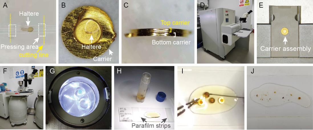
Figure 1. Sample preparation using high pressuring and freeze-substitution. A. A haltere is aspirated into the cellulose capillary tube. B. A sample capsule is transferred into the cavity of the membrane carrier filled up with cryoprotectant. C. A carrier assembly is formed by two membrane carriers with the sample in between. D. Side view of a Leica EM HPM100 high-pressure freezer. E. A carrier assembly is placed in a high-pressure freezer for cryo-fixation. F. Side view of a Leica EM AFS2 freeze-substitution device. G. A microtube containing freeze-substitution solution and samples is placed into an automatic freeze-substitution device for substitution. H. A Teflon-coated slide is wrapped with parafilm strips at both its sides. I. The samples are separated apart from the membrane carriers using forceps and a fine tip needle. J. After polymerization, the samples are flat embedded in the resin layer.Cut along the cutting line to produce a small sample capsule (<1.4 mm long) to fit the membrane carrier.
Place a 100 μm deep membrane carrier onto a filter paper with the flat side down and add 20% BSA as cryoprotectant into the cavity of the carrier. Immediately transfer the sample capsule into the cavity and immerse it into the cryoprotectant (Figure 1B).
Place another carrier with the flat side down onto the first carrier and carefully press the top carrier down to close the carrier assembly (Figure 1C). The overflow of cryoprotectant is carefully soaked away using a wedge of absorbent paper.
Critical: Air bubbles will affect pressure transmission and compromise the freezing quality. Ensure that the membrane carrier is slightly overloaded with cryoprotectant to prevent any air inclusion inside the carrier.
Once the top carrier is in place, immediately transfer the carrier assembly to a high-pressure freezer like Leica EM HPM100 to freeze the sample (Figure 1D and E).
Note: The operating manual of this machine provides a complete, detailed freezing process and we will not describe it here. Be sure to read the operating manual carefully and be trained before use.
Pause point: The frozen samples can be stored in liquid nitrogen for several months.
Under liquid nitrogen, transfer the carriers into 2 mL screwcap microtubes (<10 carriers per microtube) containing 1 mL of liquid nitrogen–precooled freeze-substitution solution and immerse the microtubes into the liquid nitrogen.
Transfer these microtubes to the precooled (-90 °C) automatic freeze-substitution device (Figure 1F and G).
Critical: The freeze-substitution solution will expand during the process of freeze-substitution as the temperature will rise. In order to relieve pressure, be sure to loosen the microtube cap or poke a hole on the cap.
Perform freeze-substitution using the following program: incubate at -90 °C for 40 h, warm gradually from -90 °C to -30 °C at a rate of 5 °C per hour, incubate at -30 °C for 8 h, warm up to 0 °C at the rate of 5 °C per hour, and keep at 0 °C for 1–6 h.
Infiltration and flat embedding
Freshly prepare a mixture of embedding media and anhydrous acetone with the ratio of 1:3, 1:1, and 3:1 (vol/vol) at room temperature and mix until homogeneous.
When the substitution program comes to 0 °C, transfer the microtubes on ice.
Wash the samples in ice-cold anhydrous acetone three times for 3 min and in anhydrous acetone at room temperature three times for 3 min.
After washing, infiltrate the samples with 1:3, 1:1, and 3:1 embedding media/acetone mixture and infiltrate for 1 h at each step at room temperature.
Replace the mixture with pure embedding media and infiltrate for overnight.
Change the pure embedding media and infiltrate for another 5–8 h on a tube revolver at room temperature.
During infiltration, prepare Teflon-coated slides, which are made by dipping the glass slides into Teflon solution for seconds, allowing them to dry in the air, and cleaning with Kimwipe tissues for use.
Critical: Be sure to use the Teflon-coated slides as they are easier to break from the polymerized embedding media.
Wrap both sides of the Teflon-coated slide with a stack of two thin strips of parafilm and flatten the parafilm strips with the fingers (Figure 1H).
Add a big drop of pure embedding media onto the center of the Teflon-coated slide and transfer all the carriers and samples into the resin drop under a stereoscope.
With a firm clamp on the carriers by forceps, slowly scrape the rim of the carrier cavity and separate the samples from the cavity using a fine tip needle (Figure 1I).
Remove all the empty carriers and place another Teflon-coated slide onto the first slide with the parafilm strips as spacer.
Critical: The Teflon-coated slides can be replaced by ACLAR® 33C film. Note that the aclar film easily bends and causes the non-uniform thickness of the layer of the embedding media. Therefore, be sure to place the aclar film onto a glass slide to avoid bending.
Transfer the sandwiched slides in an oven to polymerize the embedding media at 60 °C for at least 48 h.
After polymerization, separate the sandwiched slides using a single-edge razor blade and store the slides in a slide storage box (Figure 1J).
Pause point: After polymerization, the samples are stable indefinitely under moisture-free conditions at room temperature.
Serial sectioning
Casting formvar-coated grids
Prepare 1%–3% formvar casting solution before use.
Wash copper slot grids with anhydrous acetone and transfer these grids to a new 100 mm Petri dish lined with filter paper. Let these grids air dry and then cover the dish with its lid.
Use a cylindrical funnel with a velocity controller or a casting film device to cast formvar.
Close the velocity controller and fill casting solution nearly to the top (Figure 2A).
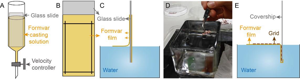
Figure 2. Casting formvar-coated grids. A. A glass slide is placed into a cylindrical funnel almost filled with formvar casting solution. B. Four cutting lines on formvar film coating are made using a single-edge razor blade. C. The formvar film coating on the glass slide detaches from the glass slide and then floats onto the water surface. D. The grids are placed onto the formvar film with the light-colored side facing up. E. The formvar film along with grids adheres to the coverslip when the coverslip is plunged into the water.Clean a glass slide with Kimwipe tissue and place it inside the cylindrical funnel.
Open the velocity controller and allow the formvar casting solution to drain with a steady flow.
Leave the glass slide in the cylindrical funnel for a few seconds and then air dry. Finally, the surface of the glass slide is coated with a thin layer of formvar film (Figure 2B).
Critical: For a selected cylindrical funnel and prepared formvar casting solution, the faster the drainage rate, the thicker the formvar film, and vice versa. Therefore, we recommend adjusting the drainage rate to control the thickness of the formvar film.
Fill up a big container with ultrapure water and clean the water surface by spreading out a Kimwipe tissue on the water surface and then dragging it across the water surface.
Use a single-edge razor blade to cut four lines parallel to the four edges of the slide on the formvar film coating (Figure 2B).
Blow a breath on the rectangle and slowly dip the slide into the ultrapure water. The formvar film coating on the rectangle comes off the glass slide and floats on the water surface (Figure 2C).
Critical: The formvar film shows a difference in color under an incandescent light when floating on the water surface. A purple, blue, or green color signifies that the formvar film is too thick and will affect the contrast of tilt-series images. Silver or grey color suggests that the formvar film is too thin and breaks easily while acquiring tilt series under a TEM. In order to meet the imaging requirements, we recommend using formvar film coating with light-gold or dark-gold color.
Use forceps to place the washed grids onto the formvar film with the light-colored side (rough side) facing up (Figure 2D).
Place a clean glass coverslip or a sheet of parafilm against the edge of the formvar film and plunge the coverslip or parafilm vertically into the water (Figure 2E). The formvar film along with grids is stuck to the surface of coverslip or parafilm.
Slowly lift the coverslip or parafilm out of the water and transfer it into a 100 mm Petri dish with grid-covered side facing up. Cover the dish with its lid and let the grids dry before use.
Poke a few holes around the outer rim of the grids and then scratch carefully along the outer rim using the tip of the forceps. Finally, pick up the formvar-coated grids with forceps and transfer the grids into a grid storage box.
Serial sectioning
Cut the sample out from the polymerized embedding media and mount the sample block onto a blank resin block using cyanoacrylic adhesive.
Note: Serial sectioning technique involves a great deal of skill. Users unfamiliar with this technique are advised to work with a skilled operator.
Under an ultramicrotome (Figure 3A and B), roughly trim the sample block to a pyramid frustum using a double-edge razor blade (Figure 3C).
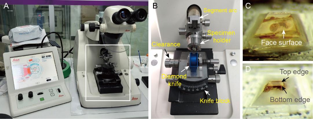
Figure 3. Sample trimming. A and B. Side view of an ultramicrotome (A); the white box in (A) indicates the enlarged region shown in (B). C. The sample block is roughly trimmed to a pyramid frustum. D. The pyramid frustum is finely trimmed to a smaller one with parallel top and bottom edges on the block face surface.Set the angle of the segment arc to 0°, clearance angle to 6°, and knife block to 0°.
Smooth the block face surface by repeated removal of 200 nm sections from the surface using a glass knife.
Finely trim the pyramid frustum to a smaller one using a double-edge razor blade (Figure 3D).
Critical: Straight section ribbons are ideal for pickup. Therefore, ensure that the top and bottom edges on the face surface are as parallel as possible because this is a must to produce a straight section ribbon.
Install a 35° diamond knife on knife block and manually move the knife block northward until the knife edge is very close to the block face surface.
Switch on the backlight of the ultramicrotome only.
Carefully move the diamond knife in east-west and north-south directions and move the sample block up and down until a band of reflected light appears on the block face surface (Figure 4A ).
Orientate the angle of the knife block until the top and bottom edges of the band of reflected light are parallel (Figure 4A).
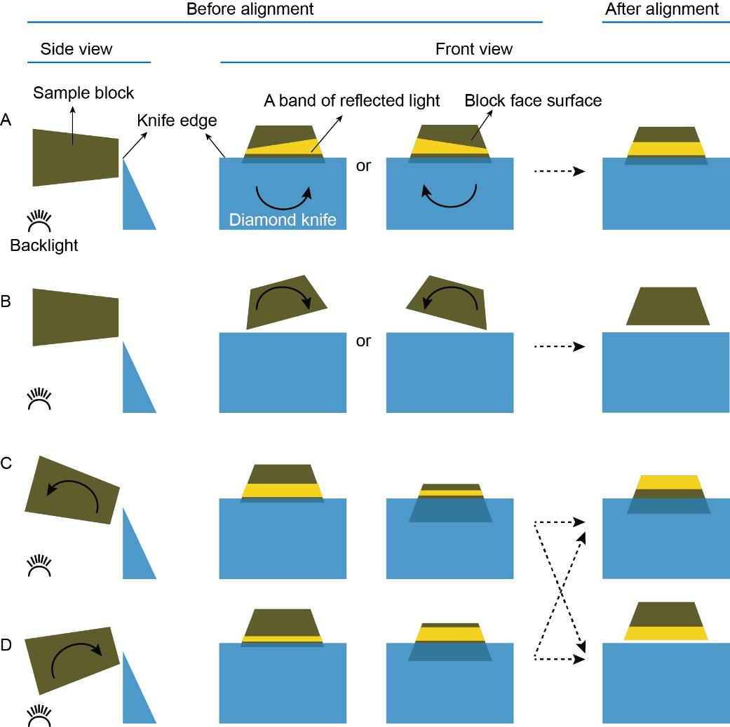
Figure 4. Schematic drawing of the alignment process between the sample block and diamond knife. A. When the sample block is very close to the knife edge, a band of reflected light appears on the block face surface under the illumination of the backlight. Orientate the knife block (the knife is accordingly rotated in the direction indicated by the curved arrows) until the top and bottom edges of the band of reflected light are exactly parallel with each other. B. When the sample block is slightly higher than the knife edge, there is a gap between the bottom edge of the block face and the knife edge. Orientate the specimen holder (the sample block is accordingly rotated in the direction as indicated by the curved arrows) until the bottom edge of the block face surface is exactly parallel to the knife edge. C and D. Move the sample block to the positions so that a band of reflected light appears again and orientate the segment arc (the sample block is accordingly rotated in the direction as indicated by the curved arrows) until the band of reflected light remains the same width as the sample moves up and down.Move the sample above the diamond knife and orientate the specimen holder until the bottom edge of the block face surface is parallel to the knife edge (Figure 4B).
Move the sample down until a band of reflected light appears on the block face surface again and orientate the segment arc until the width of the band of reflected light does not change when moving the sample up and down (Figures 4C and D).
Repeat the alignment steps until both the block face surface and its top and bottom edges are exactly parallel to the edge of the diamond knife.
Set cut start and cut end positions and switch on the top light.
Fill the knife reservoir with ultrapure water and adjust the water level until it becomes silvery.
Set feed at 300 nm and start cutting at a high cutting speed, e.g., 20 mm/s.
As soon as the first section is cut, reduce the speed to ~1 mm/s and remain at that speed for the entire cutting process. When the length of the section ribbon is suitable for the grid slot, stop cutting and use an eyelash tool to gently touch the knife edge to separate the section ribbon from the knife edge (Figure 5A).
Critical: As soon as the section ribbon is separated, immediately begin to cut the next ribbon. Otherwise, the first one or two sections of the next ribbon will be too thin or too thick.
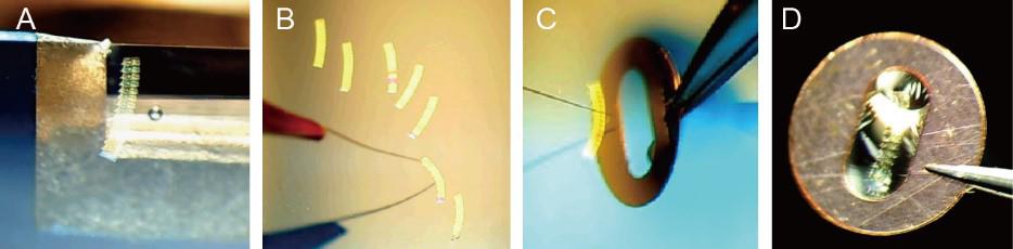
Figure 5. Pickup of section ribbons. A. A section ribbon is separated from the knife edge. B. The section ribbons float on the water surface in the knife reservoir. C. A section ribbon is picked up onto the formvar-coated grid with the help of an eyelash tool. D. A section ribbon lays flat on a formvar-coated grid.Arrange all the ribbons in the knife reservoir using an eyelash tool (Figure 5B).
Pick up the section ribbons onto formvar-coated grids (Figures 5C and D) and store the grids in a grid storage box. For pickup, clamp the grid bar with forceps, vertically dip the grid into the water with the dark-colored side (smooth side) facing to the section ribbon, and move the grid toward the ribbon or move the ribbon to the grid with the help of an eyelash tool. Once the section ribbon touches the formvar film at the center of the grid slot, slowly lift the grid and let the ribbon lay flat on the grid.
Pause point: Sections can be stored in the grid storage box for several months in dry conditions at room temperature.
Post-staining with heavy metals
Prepare 30%, 50%, and 70% aqueous methanol, 2% uranyl acetate, and 0.4% lead citrate before use.
Load the grids into the wells of the matrix body (one grid per well, up to 25 grids) of the grid-staining matrix system.
Place the matrix body into one staining vessel, add 70% aqueous methanol to completely cover all the grids for a few seconds, and replace it with 2% uranyl acetate to stain for ~10 min (Figure 6A).
Critical: At the beginning of each staining, be sure to move the matrix body back and forth several times inside the staining vessel to remove air bubbles wrapped within the wells. Otherwise, it will cause contamination of the sections.
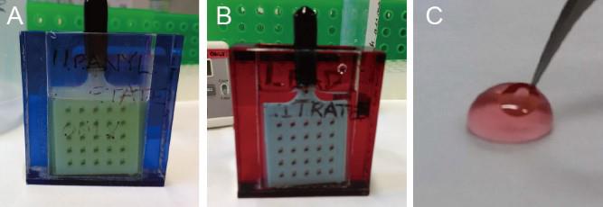
Figure 6. Post-staining. A and B. Post-staining is performed using a grid staining matrix system. The red and blue staining vessel are used for uranyl acetate or lead citrate staining, respectively. C. Gold nanoparticles are added on both sides of the sections by immersing the grid into the drop of gold nanoparticle colloid.Sequentially replace the staining solution with 70%, 50%, and 30% aqueous methanol for washing. Wash three times for each step, followed by washing with ultrapure water three times in the staining vessel and another three times in plastic beakers.
Transfer the matrix body into the other staining vessel and immediately add 0.4% lead citrate to stain for ~5 min (Figure 6B). Then, wash with ultrapure water three times in the staining vessel and another three times in plastic beakers.
Take the matrix body out, dry it with Kimwipe tissues, and carefully transfer the grids back into the grid storage box.
Critical: The application of post staining with soluble heavy metal–containing negative staining salts before imaging is indispensable for significantly improving the image contrast.
Pipette 100 μL of gold colloid into a 0.2 mL tube, vortex for a few seconds, centrifuge at ~295× g for 30 s at room temperature, and pipette the supernatant into a new 30 mm Petri dish.
Clamp the grid bar with forceps, dip the grid into the drop of supernatant for 10–30 s (Figure 6C), slowly lift the grid, carefully absorb the residual solution with a wedge of absorbent paper, and place the grid back into the grid storage box.
Critical: The gold nanoparticles serve as fiducial markers for subsequent image alignment. Be sure to check the density and distribution of gold nanoparticles in the area of interest under TEM before investing time in electron tomography. We recommend staining several times for 10 s each time until 40–100 gold particles are distributed on the surface of the area of interest.
Pause point: Sections can be stored in the grid storage box for several months in dry conditions at room temperature.
Acquisition of dual-axis tilt series
Check general conditions of TEM (Figure 7A). Here, we only describe the acquisition process using the FEI Tecnai F20 TEM equipped with Xplore3D.
Note: The tilt series in the protocol are acquired using a FEI Tecnai F20 or FEI Tecnai F30 TEM. Laboratories without this equipment can use existing TEMs equipped with automated acquisition software to achieve this purpose.
Critical: Microscope training is required before users are allowed to perform TEM. Please contact microscopists for training or assisted use.
Make sure that the vacuum level of the gun, column, and camera is reasonable and that the column valves are closed (yellow is closed, gray is open).
Fill up the Dewar flask with liquid nitrogen to cool down the Cold Trap.
Start the TEM User Interface, Digital Micrograph, and TEM Imaging and Analysis software if they are closed.
Make sure high tension is on and the value of the high tension is at 200 kV.
Make sure the FEG Control parameters are set correctly (e.g., extraction voltage is 3950 V and gun lens is 3).
Load the grid on the tomography single-tilt holder and insert the holder into the microscope.
Critical: Dual-axis tilt series are collected by tilting the object around two approximately orthogonal tilt axes (x- and y-axis, respectively) [22,23]. Be sure to load the grid on the holder with a constant orientation (Figures 7B, C, and D). Otherwise, data processing about stitching consecutive sections is going to be a problem.
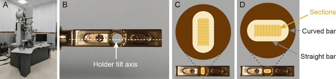
Figure 7. The grid loaded on the tomographic holder with a constant orientation. A. Side view of a transmission electron microscope (TEM). B. The tip of a tomographic holder. C and D. The grid loaded on holder with a constant orientation. There are grid sides, grid bars, and sections that can be used as orientation indicators. To acquire first tilt series, for example, the grid is loaded on the holder with the dark-colored side (smooth side) facing up, the straight bar perpendicular to the long axis of the holder (holder tilt axis), and the top edges of sections facing forward (C). Rotate the grid 90° clockwise for acquisition of second tilt series (D).Select a lower magnification (e.g., ~2,000×) and set spot size 1.
Click the Col. Valves Closed button to open the column. The beam should now be visible on the main screen. Adjust the intensity to spread the beam over the screen.
Scan across the grid to locate an area of interest and then center the beam.
Go to a higher magnification (e.g., 100,000×) and bring the area of interest to eucentric height.
Insert a selected condenser aperture and center it.
Correct condenser astigmatism to ensure the beam is round and expands concentrically.
Align gun tilt (optional), gun shift, beam tilt pp X/Y, beam shift, and rotation center.
Insert a selected objective aperture and center it.
Correct the objective astigmatism and focus the image.
Go back to a lower magnification (e.g., ~2,000×) and spread the beam out to fill the screen.
Center the area of interest and expose the sample to the beam for 2 min.
Critical: The plastic section will shrink in each dimension when viewed in electron microscope. Before data acquisition, be sure to bake the area of interest with an electron beam for inducing the rapid phase of the shrinkage so that the tilt series is recorded over the slow phase, which is tolerable for SS-ET.
Choose a working magnification (e.g., SA 29,000× resulting in a pixel size of ~1 nm).
Tilt to high angle to check what tilt range can be used without shielding the area of interest. A tilt-range of ±60° is needed for good tomography results.
Go back to zero tilt degree and use the Digital Micrograph to record images with 1 s of exposure time, binning 2 (an image has 2048 × 2048 pixels), and full image frame.
Adjust the beam intensity and defocusing until the image has good contrast and appearance. The optimal beam intensity and defocusing values are going to be used for acquiring the tilt series.
Start the Xplore 3D software; the Tomography Tasks panel comes out.
Critical: The application instructions of Xplore 3D provide a step-by-step guide for microscope users and the help file offers a detailed description of all parameter settings. Here, we just depict a typical procedure and parameters needed to acquire a good TEM tilt series at medium-high magnification.
In the Tomography Tasks panel, click the Holder Calibration and the Select View panel turn to Holder Calibration Data.
Click the button Load and load the selected hold calibration file specially created for plastic sample from the save directory into the system.
Go back to the Tomography Tasks panel, click the Acquire Tilt Series, and the Select View panel turns to Camera Acquisition Parameters.
Adjust the settings for Search, Focus, Exposure, and Tracking if necessary. For exposure mode, we recommend using full image size, binning 2, and 1 s of exposure time.
Press Apply to activate the changes and press the Proceed button to continue.
The Select View panel turns to Tilt Series Parameters. Set the parameters. Generally, Max. Negative Angle and Max. Positive angle are -60° and +60° and Start angle is -60°. Check the Continuous for the plastic section, which allows the object to be tilted from -60° to +60°. Stage relaxation time is 4–6 s, which is needed to stabilize the sample stage before focusing and exposure are performed. Choose MRC Series format for tilt series dataset and put the Series Name; note that the names of first and second tilt series are distinguished by adding the letter a or b to the same common name (e.g., “*a” for first tilt series and “*b” for second tilt series). Uncheck the Start At Eucentric Height and Start with AutoFocus since eucentric height and focus were done before. The 1° Tilt Step allows more image information to be obtained for tomographic reconstruction. Let the software do an autofocus every 4–6° at Low Tilt angle and every one degree at High Tilt (above 50–55°) for taking well-focused images. Set the Applied defocus value (e.g., -1 μm) to enhance the contrast of images. Check Track Before Acquisition to manually keep the feature of interest well centered throughout the whole tilt series.
Press Apply to activate the changes and press Proceed to automatically acquire tilt series.
Critical: The first few images at high tilts are normally of poor quality; be sure to manually center or focus the region of interest if necessary.
Wait until the acquisition of first tilt series is finished.
Go to the save directory and check the tilt series stored in a file with the suffix .mrc. Also, keep the log files (only a few kB in size) as they might help you in the future if data acquisition was not satisfactory.
Collect first tilt series for the other sections at the same working magnification.
After data acquisition, set the magnification to the lowest “M” setting, spread the beam to cover the screen, close the column valves, and pull the holder out of the microscope.
Rotate the grid by 90° clockwise and collect the second tilt series for each section at the same working magnification.
Build a dual-axis tomogram reconstruction with the Etomo program in the IMOD software package [22]. The IMOD software package and a detailed Etomo tutorial can be downloaded at the IMOD homepage. Therefore, we do not provide a comprehensive tutorial for reconstruction.
Tracing microtubules from tomographic reconstructions
Start the Amira ZIB edition 2016.16.
Click the Project button in the workroom toolbars to arrive at the Project workroom.
Load a reconstruction result with the suffix .rec into the system. Once the data object has been loaded, it is represented by a green icon in the Project View.
Click on the green data icon with the right mouse button and a popup menu appears containing all modules, which can be used to process this type of data. Choose the Slice module to display the data object in the 3D view window.
Soften the image object with a smoothing module or/and crop it using the Crop Editor module if needed.
Compute normalized cross-correlation for the image data. For computing, attach the Cylinder Correlation module to the image data, define the microtubules by setting the parameters in the Properties area, and finally press the Apply button.
After several hours of computation, two objects, i.e., “*CorrelationField.am” and “*OrientationField.am,” are produced.
Trace centerlines of microtubules. To trace, attach a Trace Correlation Lines module to the “*CorrelationField.am” object and, in the Properties area of Trace Correlation Lines module, select “*CorrelationField.am” object at the Data port and “*OrientationField.am” object in Orientation Field port to connect the two objects to the Trace Correlation Lines module.
Set all other parameters in the Properties area of Trace Correlation Lines module and finally press Apply button to proceed.
Just a few minutes later, a new object, “*CorrelationLines.am” for centerlines of microtubule, is produced and can be displayed with LineRaycast module.
Switch into the Filament workroom and edit the traced centerlines until they match exactly to the real microtubules.
Trace microtubules for the other tomographic reconstructions.
Stitching consecutive tomographic reconstructions to form a single larger volume
In the Amira ZIB edition 2016.16, switch to the Project workroom.
Right-click in the blank of the Project View area and select the Create Object. A dialog box then appears; enter and select the SerialSectionStack module in the drop-down menu. A green icon of SerialSectionStack appears in the Project view area.
Click Add Files in the Properties area of SerialSectionStack module, choose the tomographic reconstructions named “*.rec” and their corresponding microtubule objects named “*CorrelationLines.am,” and press the Open button to load these files.
Critical: After loading, ensure that the tomographic reconstructions are in the same order as their sectioning sequence and no changes are made to these reconstruction results and their corresponding microtubule objects. Otherwise, the process of stitching adjacent tomographic reconstructions cannot be performed.
Add the SerialSectionAligner module to SerialSectionStack and the 3D view window is separated into four panels. In the lower-right panel, each bar represents a tomographic reconstruction, and the blue and yellow bars represent the two working reconstructions, whose microtubules are displayed as blue or yellow dots in the upper and lower left panels and whose slices, together with these dots, are displayed in the upper-right panel.
Click the slide bars in the lower-right panel to choose the two working reconstructions.
Left-click twice in the upper-left panel and red solid circles appear on the upper- and lower-left panels.
Drag these red solid circles until the blue dots are well matched with the yellow dots.
Check Matching in the Properties area of SerialSectionAligner module.
Hold down the Ctrl key on the keyboard and left-click the matched blue and yellow dots, in the upper-right panel, to connect the two microtubule segments.
After connection, check the Alignment in the Properties area of SerialSectionAligner module and choose another two working reconstructions to complete the connection of microtubule segments in the same way mentioned above.
After all the microtubule segments are connected, press the Create button. A few minutes later, two Objects are produced, and their icons appear in the Project View area: one is an image object of stitched consecutive reconstructions and the other is a line object of connected microtubule segments.
Surface segmentation
Load the image object from the directory into the Amira ZIB edition 2016.16.
Go to the Segmentation workroom and a new green icon named “*labels.am” is created in the Project View area.
Set an appropriate magnification by pressing the zoom in and out buttons in the Zoom and Data Window region.
Draw the outlines of the same structure through all the slices using the brush. If the structure has little change among slices, draw the structure every few slices and click the Interpolate from the Selection menu bar to select the structure in between marked slices.
Note: The brush is one of the basic segmentation tools. Other segmentation tools can also be used for this job.
Select a Material in the material list and click the plus sign in the Selection region. The selected pixels in all slices are now assigned to the selected Material. Of course, more meaningful names or colors can be used to the material. The new Material can be added by pressing the New button or from the right-button menu.
Go to slices and assign the other structures into different Materials.
After drawing, add the Generate Surface module to “*labal.am” object in the Project workroom and press the Apply button. A dialog comes out; press Continue.
A few minutes later, a new icon named “*surf.am” is created and the segmentation result can be displayed with the Surface View module.
Add the Animate Ports to the Slice or other display modules and further adhere the Movie Maker module to Animate Ports.
Right-click in the blank of the Project View area to create the Camera-Orbit.
Adjust the setting of Animate Ports, Movie Maker, and Camera-Orbit to generate a movie of the segmentation results.
Measurement
In Amira ZIB edition 2016.16, left-click the Measuring Tool button at the top of the 3D view window and choose the 3D Length from the pull-down menu.
Note: There are several tools for measurement, including 2D Length, 2D Angle, 3D Angle, 3D Box, and 3D circle. Which one is selected depends on the structures that users want to measure.
Left-click one point on the object and then drag the mouse to another point in 3D space. The length of the line is shown on the 3D view window and a new icon named Measurement is created in the Project view area.
Measure all geometrical parameters of the fly MOs. These parameters can be used for further analysis.
Data analysis
In this protocol, SS-ET is used to resolve the 3D structures of fly MOs. The dual-axis tilt series are captured to reconstruct the tomogram (Figures 8A and B). Then, microtubules are traced and applied as fiducial markers to stitch the sections in z-axis (Figures 8C and D). Finally, tomograms of ten consecutive sections are combined into a single larger volume (Figure 8E). From the lateral view, the morphology of the modified cilium can be recognized (Figure 8F). In the modified cilium, the basal body is located at the base and the cilium extend from the basal body to the tubular body, which is nearly spherical. Above the distal end of the tubular body is the MO. Of note, the material loss induced by knife sectioning and distortions caused by electrons irradiation, while tolerable, are visible at the connection between sections. From the cross-sectional view of the MO, the smooth membrane, the microtubules arranged in two rows with electron-dense materials in between, and the high density of the regularly spaced membrane-microtubule connectors are all recognized (Figure 8G).
All structural measurements in 3D reconstruction were performed in Amira as described above.
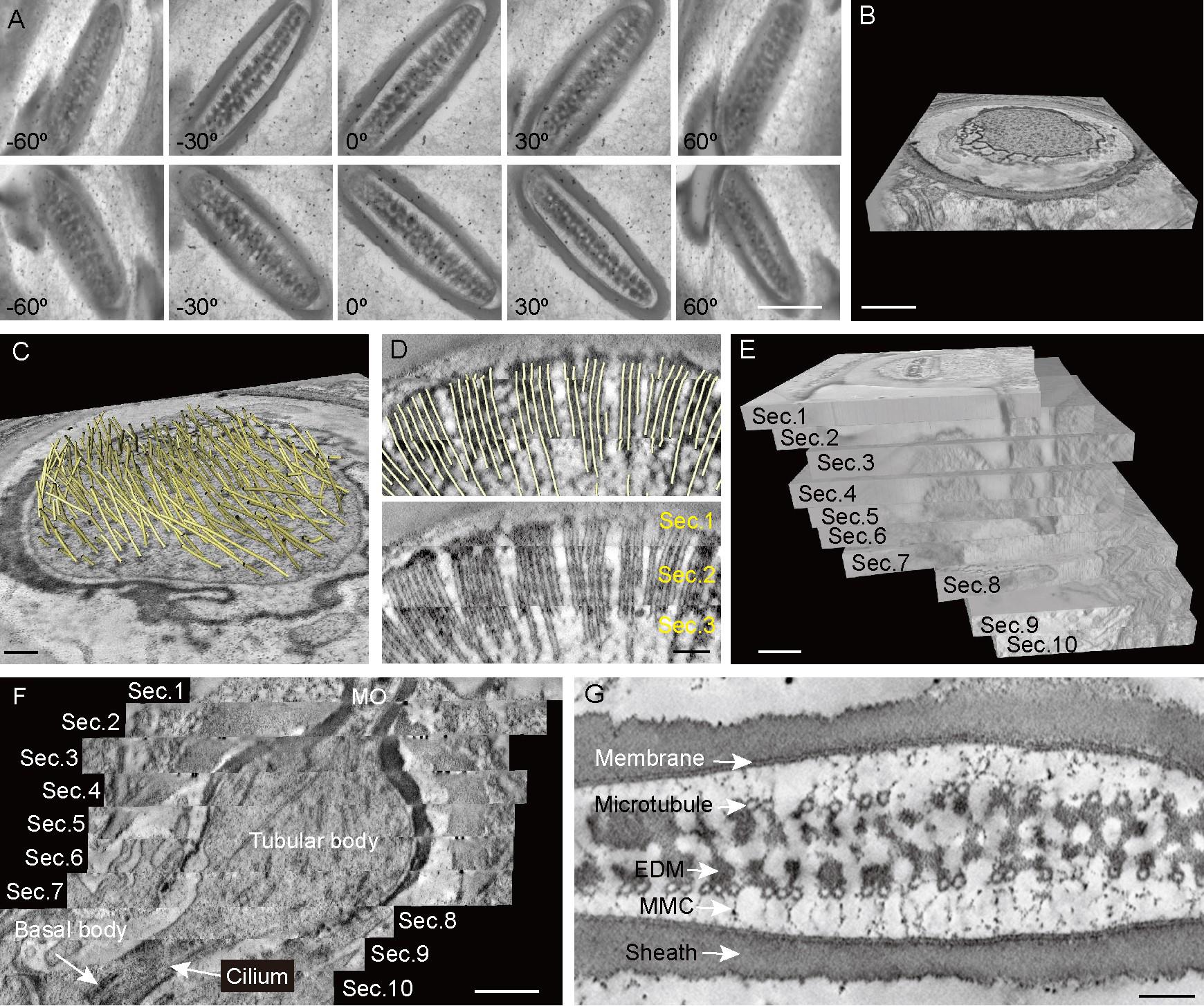
Figure 8. Representative data using the protocol. A. Several individual images at different tilt angles are from the first tilt series (upper) and second tile series (lower). Scale bar: 0.5 μm. B. Tomogram reconstructed from dual-axis tilt series. Scale bar: 0.5 μm. C. Microtubules were traced from the tomographic reconstruction. Scale bar: 100 nm. Each microtubule was shown as a yellow rod. D. Microtubules were used as fiducial markers (upper) to stitch the sections (lower) in z-axis. Scale bar: 100 nm. E. Ten consecutive sections are combined into a single larger volume. Scale bar: 0.5 μm. F. Representative lateral view of a modified cilium generated from the single larger volume. Scale bar: 0.5 μm. G. Representative cross-sectional view of a mechanosensory organelle (MO) and its internal architectures. EDM, electron-dense materials. MMC, membrane-microtubule connector. Scale bar: 100 nm.
Validation of protocol
This protocol has been used and validated in the following published articles:
Song, X. et al. (2023). DCX-EMAP is a core organizer for the ultrastructure of Drosophila mechanosensory organelles. J Cell Biol 222(10): e202209116, DOI: 10.1083/jcb.202209116.
Sun, L. D. et al. (2021). Katanin p60-like 1 sculpts the cytoskeleton in mechanosensory cilia. J Cell Biol 220(1): e202004184, DOI: 10.1083/jcb.202004184.
Sun, L. D. et al. (2019). Ultrastructural organization of NompC in the mechanoreceptive organelle of Drosophila campaniform mechanoreceptors. Proc Natl Acad Sci USA 116(15): 7343–7352, DOI: 10.1073/pnas.1819371116.
General notes and troubleshooting
General notes
We suggest that scientists implementing the protocol described here should have extensive knowledge of TEM techniques. Also, scientists should already be familiar with manipulations of preparing and handling specimens and 3D tomographic image processing software.
This protocol, with minimal adaptive modifications, could also be applied to the studies on other sensory processes, like olfaction, gustation, vision, etc. Moreover, 3D structural analysis is helpful to understand non-sensory processes, such as neuronal cytoskeleton regulations, synaptic remodeling, membrane-bound vesicle dynamics, intracellular trafficking, etc.
This protocol is still a time-consuming approach for ultramicrotomy, microscopy, and data processing; therefore, the choice of the technology must be made based on the specific biological questions.
Troubleshooting (Table 1)
Table 1. TroubleshootingIssue Possible reason Solution Failure of aspirating the sample into the cellulose capillary tube Sample with hydrophobic cuticle easily floats on the surface of aqueous solution, which, in turn, leads to the failure. Press the sample to the bottom of the droplet with forceps and make sure there are no air bubbles around the sample. Samples become black Osmium tetroxide in freeze-substitution solution forms osmium black at room temperature. Wash the samples several times with ice-cold anhydrous acetone to thoroughly remove the fixatives. Section ribbon is not formed, or section ribbons easily break into short ribbons The trimmed sample block does not meet the requirements for serial sectioning. Retrim the sample block until the top and bottom edges of block face surface are parallel. Improper alignment between block face surface and diamond knife. Repeat the alignment process to make the alignment perfect. Diamond knife is contaminated with hydrophobic substances such as oil from hands. Thoroughly clean the knife with 70% alcohol. Poor contrast after post-staining Different sources of heavy metals. Select the optimal staining time for 2% uranyl acetate and 0.4% lead citrate. Contamination of sections Precipitates occur in the heavy metal solution. Filter or centrifuge the solution, then collect the filtrate or supernatant to use.
Acknowledgments
The authors thank members of the Cell Biology Facility and Electron Microscopy Facility of Tsinghua University for technical support. This work was supported by National Natural Sciences Foundation of China (32370730, 32070704 and 32350029).
Competing interests
The authors declare that they have no competing interests.
References
- Gillespie, P. G. and Walker, R. G. (2001). Molecular basis of mechanosensory transduction. Nature 413(6852): 194–202. https://doi.org/10.1038/35093011
- Lumpkin, E. A., Marshall, K. L. and Nelson, A. M. (2010). The cell biology of touch. J. Cell Biol. 191(2): 237–248. https://doi.org/10.1083/jcb.201006074
- Singhania, A. and Grueber, W. B. (2014). Development of the embryonic and larval peripheral nervous system of Drosophila. WIREs Dev. Biol. 3(3): 193–210. https://doi.org/10.1002/wdev.135
- Chalfie, M. (2009). Neurosensory mechanotransduction. Nat. Rev. Mol. Cell Biol. 10(1): 44–52. https://doi.org/10.1038/nrm2595
- Cueva, J. G., Mulholland, A. and Goodman, M. B. (2007). Nanoscale organization of the MEC-4 DEG/ENaC sensory mechanotransduction channel in Caenorhabditis elegans touch receptor neurons. J. Neurosci. 27(51): 14089–14098. https://doi.org/10.1523/jneurosci.4179-07.2007
- Effertz, T., Nadrowski, B., Piepenbrock, D., Albert, J. T. and Göpfert, M. C. (2012). Direct gating and mechanical integrity of Drosophila auditory transducers require TRPN1. Nat. Neurosci. 15(9): 1198–1200. https://doi.org/10.1038/nn.3175
- Gillespie, P. G. and Müller, U. (2009). Mechanotransduction by hair cells: models, molecules, and mechanisms. Cell 139(1): 33–44. https://doi.org/10.1016/j.cell.2009.09.010
- Keil, T. A. (1997). Functional morphology of insect mechanoreceptors. Microsc. Res. Tech. 39(6): 506–531. https://doi.org/10.1002/(sici)1097-0029(19971215)39:6<506::aid-jemt5>3.0.co;2-b
- Liang, X., Madrid, J., Gärtner, R., Verbavatz, J. M., Schiklenk, C., Wilsch-Bräuninger, M., Bogdanova, A., Stenger, F., Voigt, A., Howard, J., et al. (2013). A NOMPC-dependent membrane-microtubule connector is a candidate for the gating spring in fly mechanoreceptors. Curr. Biol. 23(9): 755–763. https://doi.org/10.1016/j.cub.2013.03.065
- Liang, X., Sun, L. and Liu, Z. (2017). Mechanosensory transduction in drosophila melanogaster. SpringerBriefs in Biochemistry and Molecular Biology: e1007/978–981–10–6526–2. https://doi.org/10.1007/978-981-10-6526-2
- Sun, L., Gao, Y., He, J., Cui, L., Meissner, J., Verbavatz, J. M., Li, B., Feng, X. and Liang, X. (2019). Ultrastructural organization of NompC in the mechanoreceptive organelle of Drosophila campaniform mechanoreceptors. Proc. Natl. Acad. Sci. U.S.A. 116(15): 7343–7352. https://doi.org/10.1073/pnas.1819371116
- Keil, T. A. (2012). Sensory cilia in arthropods. Arthropod Structure & Development 41(6): 515–534. https://doi.org/10.1016/j.asd.2012.07.001
- Liang, X., Madrid, J. and Howard, J. (2014). The microtubule-based cytoskeleton is a component of a mechanical signaling pathway in fly campaniform receptors. Biophys J. 107(12): 2767-2774. https://doi.org/10.1016/j.bpj.2014.10.052
- Thurm, U., Erler, G., Godde, J., Kastrup, H., Keil, T., Volker, W. and Vohwinkel, B. (1983). Cilia specialized for mechanoreception. J. Submicrosc. Cytol. Pathol. 15(1): 151-155. https://royalsocietypublishing.org/doi/10.1098/rstb.2019.0376
- Zhang, W., Cheng, L. E., Kittelmann, M., Li, J., Petkovic, M., Cheng, T., Jin, P., Guo, Z., Göpfert, M. C., Jan, L. Y., et al. (2015). Ankyrin repeats convey force to gate the NOMPC mechanotransduction channel. Cell 162(6): 1391–1403. https://doi.org/10.1016/j.cell.2015.08.024
- Song, X., Cui, L., Wu, M., Wang, S., Song, Y., Liu, Z., Xue, Z., Chen, W., Zhang, Y., Li, H., et al. (2023). DCX-EMAP is a core organizer for the ultrastructure of Drosophila mechanosensory organelles. J. Cell Biol. 222(10): e202209116. https://doi.org/10.1083/jcb.202209116
- Sun, L., Cui, L., Liu, Z., Wang, Q., Xue, Z., Wu, M., Sun, T., Mao, D., Ni, J., Pastor-Pareja, J. C., et al. (2020). Katanin p60-like 1 sculpts the cytoskeleton in mechanosensory cilia. J. Cell Biol. 220(1): e202004184. https://doi.org/10.1083/jcb.202004184
- Baumeister, W. (2002). Electron tomography: towards visualizing the molecular organization of the cytoplasm. Curr. Opin. Struct. Biol. 12(5): 679–684. https://doi.org/10.1016/s0959-440x(02)00378-0
- Lučić, V., Förster, F. and Baumeister, W. (2005). Structural studies by electron tomography: From Cells to Molecules. Annu. Rev. Biochem. 74(1): 833–865. https://doi.org/10.1146/annurev.biochem.73.011303.074112
- Soto, G. E., Young, S. J., Martone, M. E., Deerinck, T. J., Lamont, S., Carragher, B. O., Hama, K. and Ellisman, M. H. (1994). Serial section electron tomography: A method for three-dimensional reconstruction of large structures. NeuroImage 1(3): 230–243. https://doi.org/10.1006/nimg.1994.1008
- Toyooka, K. and Kang, B. H. (2013). Reconstructing plant cells in 3D by serial section electron tomography. Methods Mol. Biol. : 159–170. https://doi.org/10.1007/978-1-62703-643-6_13
- Mastronarde, D. N. (1997). Dual-axis tomography: An approach with alignment methods that preserve resolution. J. Struct. Biol. 120(3): 343–352. https://doi.org/10.1006/jsbi.1997.3919
- Penczek, P., Marko, M., Buttle, K. and Frank, J. (1995). Double-tilt electron tomography. Ultramicroscopy 60(3): 393–410. https://doi.org/10.1016/0304-3991(95)00078-x
Article Information
Copyright
© 2024 The Author(s); This is an open access article under the CC BY-NC license (https://creativecommons.org/licenses/by-nc/4.0/).
How to cite
Readers should cite both the Bio-protocol article and the original research article where this protocol was used:
- Sun, L., Meissner, J., He, J., Cui, L., Fürstenhaupt, T. and Liang, X. (2024). Resolving the In Situ Three-Dimensional Structure of Fly Mechanosensory Organelles Using Serial Section Electron Tomography. Bio-protocol 14(4): e4940. DOI: 10.21769/BioProtoc.4940.
- Song, X., Cui, L., Wu, M., Wang, S., Song, Y., Liu, Z., Xue, Z., Chen, W., Zhang, Y., Li, H., et al. (2023). DCX-EMAP is a core organizer for the ultrastructure of Drosophila mechanosensory organelles. J. Cell Biol. 222(10): e202209116. https://doi.org/10.1083/jcb.202209116
Category
Biophysics > Electron cryotomography > 3D image reconstruction
Cell Biology > Cell structure > Cell organelle
Do you have any questions about this protocol?
Post your question to gather feedback from the community. We will also invite the authors of this article to respond.