CoCoNat: A Deep Learning–Based Tool for the Prediction of Coiled-coil Domains in Protein Sequences

Matteo  Manfredi; Castrense  Savojardo; Pier Luigi  Martelli; Rita  Casadio

doi:10.21769/BioProtoc.4935

Improve Research Reproducibility A Bio-protocol resource

Submit a Protocol
Receive Our Alerts
EN
- EN - English
- CN - 中文

Peer-reviewed

CoCoNat: A Deep Learning–Based Tool for the Prediction of Coiled-coil Domains in Protein Sequences

MM Matteo Manfredi

CS Castrense Savojardo

PM Pier Luigi Martelli email

RC Rita Casadio

Published: Vol 14, Iss 4, Feb 20, 2024 DOI: 10.21769/BioProtoc.4935 Views: 1531

Reviewed by: Prashanth N SuravajhalaAnonymous reviewer(s)

Download PDF

Ask a question

How to cite

Favorite

Cited by

Original research article

The authors used this protocol in:

Cover of Bioinformatics, featuring study using the protocol.

Aug 2023

Protocol Collections

Cell Imaging - A Special Collection for Cell Bio 2023

See all

Abstract

Coiled-coil domains (CCDs) are structural motifs observed in proteins in all organisms that perform several crucial functions. The computational identification of CCD segments over a protein sequence is of great importance for its functional characterization. This task can essentially be divided into three separate steps: the detection of segment boundaries, the annotation of the heptad repeat pattern along the segment, and the classification of its oligomerization state. Several methods have been proposed over the years addressing one or more of these predictive steps. In this protocol, we illustrate how to make use of CoCoNat, a novel approach based on protein language models, to characterize CCDs. CoCoNat is, at its release (August 2023), the state of the art for CCD detection. The web server allows users to submit input protein sequences and visualize the predicted domains after a few minutes. Optionally, precomputed segments can be provided to the model, which will predict the oligomerization state for each of them. CoCoNat can be easily integrated into biological pipelines by downloading the standalone version, which provides a single executable script to produce the output.

Key features

• Web server for the prediction of coiled-coil segments from a protein sequence.

• Three different predictions from a single tool (segment position, heptad repeat annotation, oligomerization state).

• Possibility to visualize the results online or to download the predictions in different formats for further processing.

• Easy integration in automated pipelines with the local version of the tool.

Graphical overview

Keywords: Coiled-coil segments

Oligomerization

Deep learning

Prediction

Protein Language Models

Web server

Background

Coiled-coil domains (CCDs) are structural motifs where α‐helices pack together in an arrangement called knobs-into-holes [1], by which residues from one helix (the knobs) pack into holes formed by side chains in the other helices participating in the domain. CCDs have been observed in different kinds of proteins sequenced from all the kingdoms of life [2] and perform a great number of diverse functions.

Canonical CCDs include the interaction of two or more α‐helices, each characterized by the repetition of a seven-residue motif called heptad repeat. The positions of the heptad repeat are referred to as registers and are labeled with the letters a–g. CCDs can be classified into different oligomerization states, depending on the number (dimers, trimers, tetramers, and higher orders) and orientation (parallel or antiparallel) of the involved α‐helices.

Methods such as SOCKET [3] or SamCC-Turbo [4] can annotate CCDs starting from the experimental 3D structure of a protein. In the absence of structural information, several tools have been proposed over the years to perform automatic annotations on protein sequences, each addressing different tasks of CCD prediction (i.e., segment localization, heptad repeat annotation, oligomerization state classification).

Recently, the development of protein language models (PLMs) introduced a novel way of generating embeddings to encode protein sequences for downstream predictive tasks. We proposed CoCoNat [5], a deep learning–based approach that exploits two different and complementary PLMs, ProtT5 [6] and ESM2 [7], to produce a predictive pipeline for the complete ab initio annotation of CCDs.

CoCoNat processes input sequences with three cascading networks, each trained independently to solve a specific task. The first step adopts a deep architecture based on convolutional and recurrent layers to identify the presence of coil-coiled segments along the sequence. The second step adopts a probabilistic graphical model to assign registers to each residue in the segment. Finally, the third step adopts a neural network to predict the oligomerization state of each segment. Each prediction is also complemented with the probabilities computed by the network, allowing users to assess their reliability.

CoCoNat is trained on a dataset comprising 2,198 proteins annotated with 4,342 helices and 9,062 proteins without CCD. When tested on a non-redundant benchmark dataset, comprising 400 proteins annotated with 863 helices and 318 proteins without CCD, CoCoNat outperforms other methods on all three predictive tasks included in the pipeline. Specifically, it achieves a 0.54 per-residue F1 score and a 0.49 per-segment F1 score on the identification of segment boundaries over the sequence (first step in the Graphical overview), a Matthew's Correlation Coefficient (MCC) between 0.83 and 0.84 for each type of register in the annotation of the heptad repeats (second step in the Graphical overview), and an average MCC of 0.58 for the 4-class classification of the oligomerization state (third step in the Graphical overview).

Moreover, the adoption of PLMs to encode the input allows CoCoNat to be extremely time efficient. When tested on the virtual machine hosting the web server (AMD EPYC 7301 12-Core Processor, 48 GB RAM, no GPU), CoCoNat requires an average running time of 330 s (5.5 min) to predict 100 sequences of length comprised between 100 and 200 residues. The same computation takes approximately 2.5 h with CoCoPRED [8], a similar tool based on canonical multiple sequence alignments.

Here, we illustrate in detail how CoCoNat can be adopted as a web server or as a standalone tool, allowing for easy integration into any computational pipeline. As a test case, we select one of the proteins belonging to our benchmark dataset, the Mating-type switching protein swi5 from the organism Schizosaccharomyces pombe (UniProt accession: Q9UUB7). This protein presents two coiled-coil segments organized as a parallel dimer that CoCoNat identifies. Both the registers and the oligomerization classes are correctly assigned. The only difference between the putative and the real annotations is the length of the segments.

Supplementary File S1 reports a schema of the web server compliant with the Minimum Information About Bioinformatics investigation (MIABi) guidelines [9].

Equipment

Computer with internet access and a web browser
(Only for online execution) CoCoNat web server (https://coconat.biocomp.unibo.it/)
(Only for local execution) Machine with a macOS or Linux operating system and at least 4 CPU cores and 48 GB of RAM
The local release is not suitable to be executed directly on a machine with a Windows operating system. In this case, the adoption of a virtual machine or the Windows Subsystem for Linux (WSL) is recommended.

Software and datasets

Docker Engine, installed (https://docs.docker.com/engine/install/debian/)
Miniconda, installed (https://docs.conda.io/projects/miniconda/en/latest/miniconda-install.html)
As long as Miniconda is installed, Python 3 and pip (both mentioned in the protocol) do not need to be installed separately, as they will be included in the environment generated by Miniconda.

Procedure

Online single sequence prediction
1. Prepare your sequence in FASTA format.
2. Open the homepage of the web server (https://coconat.biocomp.unibo.it/).
3. Paste your sequence in the form or upload the FASTA file.
4. The web server will validate the format of your input. If the limitations are too strict for your target sequence, we suggest following Procedure C and running CoCoNat locally.
  1. Valid FASTA format.
  2. Sequence length between 40 and 700 residues.
  3. Contains only 20 standard amino acids, 3 non-standard residues (UZB), or undetermined character (X).
5. (Optional) Provide precomputed coiled-coil segments.
  1. Tick the box Provide precomputed coiled-coil segments (predict only oligomerization state).
  2. Paste sequence of states. Use the letter i to indicate a residue that is not part of a coiled-coil segment; use the letters a–g to indicate the registers of the residues in the coiled-coil segment.
  3. If you only know the segments but not the registers, skip this step and run the full prediction.
6. Press Submit (Figure 1).
  
  Figure 1. Online single sequence submission page. Homepage of the CoCoNat web server, where users can submit a target sequence in FASTA format. It is possible to load an example sequence (1) or to upload a file from the computer (2). Optionally, it is possible to provide precomputed coiled-coil segments. A button loads an example (3) showing the correct format. At the end of the page, it is possible to clear the forms (4) or to submit the job to start the prediction (5).
7. Bookmark the page that loads after job submission. This page will be updated with the results as soon as they are ready.
8. Graphically visualize the results (Figure 2).
  1. Under Predicted coiled-coil segments, you will see a list of all predicted segments, including the following information:
    i. Segment start.
    ii. Segment end.
    iii. Length of segment.
    iv. Predicted registers.
    v. Predicted oligomerization state.
    
    Figure 2. Online single sequence result page (full prediction). Results are visualized after submitting the example input to the web server, without precomputed segments. From the results page, it is possible to copy the link (1) to access them at a later date and to download the results in tab-separated values (TSV) format (2) or in JSON format (3). For each predicted segment, clicking on the magnifying glass (4) will zoom in the corresponding region on the sequence feature viewer. The viewer itself offers the possibility to change visualization by zooming in or out, resetting the zoom, and moving along the sequence length (5). Finally, it is possible to save a screenshot of the selected portion of the sequence (6).
  2. Under Sequence feature view, you will see four lines visualizing from top to bottom the following data:
    i. Residue sequence.
    ii. Predicted coiled-coil regions (colored depending on the predicted oligomerization state).
    iii. Predicted registers (colored depending on the register type).
    iv. Coiled-coil probability, showing how confident the model is at each position.
  3. (Optional) If you provided precomputed coiled-coil segments (see step A5), the coiled-coil probabilities (see steps A8b–8d) will be all equal to 1, and only the oligomerization state will be predicted by the web server (Figure 3).
  4. If needed, a button is available to take screenshots of the selected region of the sequence.
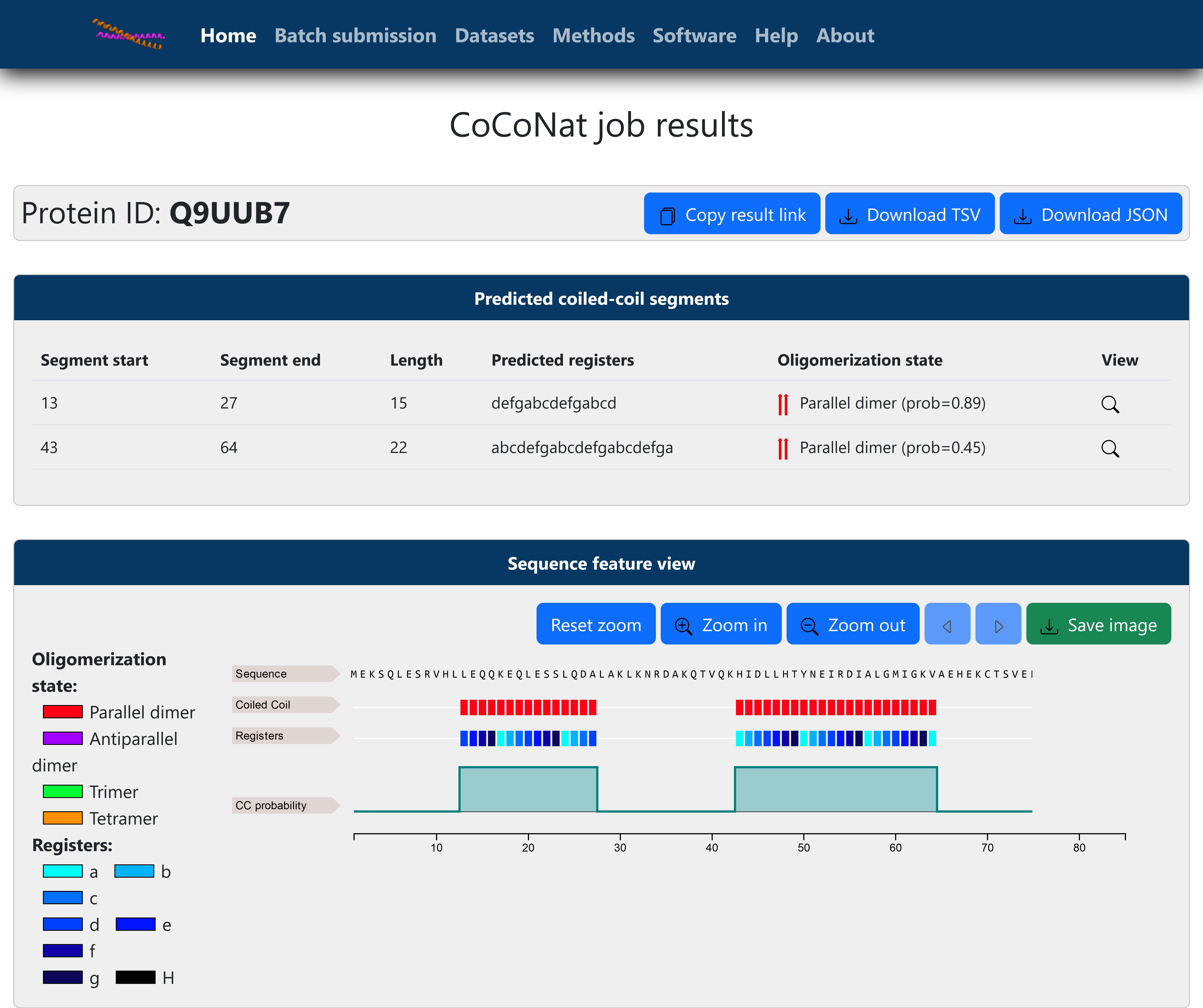
  Figure 3. Online single sequence result page (precomputed segments). Results are visualized after submitting the example input to the web server. In this case, only the oligomerization state was predicted, and the precomputed segments are visualized with an associated probability equal to 100%. The functionalities of the web server are the same as detailed in Figure 2.
9. Download results with the buttons at the top of the page.
  1. If you select the tab-separated format (TSV), the generated file will contain a line for each residue (plus the header) organized in 14 columns, containing information about:
    i. ID: ID of the protein.
    ii. RES: Residue type.
    iii. CC_CLASS: Predicted coiled-coil class. The coiled-coil class is i if the residue does not belong to a coiled-coil segment; otherwise, it is a letter from a to g that indicates the predicted register.
    iv. OligoState: Predicted oligomerization state (P, A, 3, or 4 for parallel dimer, antiparallel dimer, trimer, or tetramer, respectively).
    v. Pi, Pa-Pg, PH: nine columns for the computed probabilities for each possible coiled-coil class (the higher probability will determine the content of the third column).
    vi. pOligo: Computed probability of the predicted oligomerization state reported in point iv (the higher the probability, the higher the confidence of the model).
  2. If you select the JSON format, the generated file will contain one entry with 10 fields:
    i. accession: ID of the protein.
    ii. res: FASTA sequence.
    iii. labels: Sequence of predicted coiled-coil classes (see step A9a.iii).
    iv. prob: List of probabilities assigned by the predictor to the most likely coiled-coil class for each residue.
    v. oligo: Sequence of predicted oligomerization classes (see step A9a.iv).
    vi. prob_oligo: List of probabilities assigned by the predictor to the most likely oligomerization class for each residue.
    vii. segments: List with one item for each predicted segment reporting summary information about it.
    viii. length: Length of the protein.
10. A typical computation for a single sequence prediction will require approximately 90 s (1.5 min).
11. For further help and details, please reference the Help page of the web server (https://coconat.biocomp.unibo.it/help/).

Online batch prediction
1. Prepare your sequences in FASTA format.
2. Open the Homepage of the web server and go to the tab batch submission (https://coconat.biocomp.unibo.it/batch/).
3. Upload the FASTA file.
4. (Optional) Provide an email address. When results are ready, the link to access them will be sent to you.
5. The web server will validate the format of your input. If the limitations are too strict for your target sequences, we suggest following Procedure C and running CoCoNat locally.
  1. Valid FASTA format.
  2. No more than 500 sequences.
  3. All sequences with length between 40 and 700 residues and total number of residues not greater than 80,000.
  4. Each sequence contains only 20 standard amino acids, 3 non-standard residues (UZB), or undetermined character (X).
6. Press Submit.
7. Bookmark the page that loads upon job submission. This page will be updated with the results as soon as they are ready. If you have provided an email address, you will receive the link to this page via email once the results are ready.
8. Download results with the buttons at the top of the page.
  1. See Procedure A, step 9a for a description of the TSV format.
  2. See Procedure A, step 9b for a description of the JSON format. Mind that, in this case, the JSON file will contain one entry for each sequence in the input file.
9. The time needed for computing the outputs will depend on the number and length of the input sequences. A job containing 100 sequences with lengths between 100 and 200 residues should take approximately 330 s (5.5 min).
10. For further help and details please reference the Help page of the web server (https://coconat.biocomp.unibo.it/help/).

Local prediction
Note: All lines of code reported in this section are meant to be executed inside a terminal.
1. Prepare the environment (see Figure 4).
  1. Create a conda environment with Python 3.
    
    conda create -n coconat python
    conda activate coconat
  2. Install dependencies using pip.
    
    pip install docker absl-py
  3. Clone locally the GitHub repository in your current working directory; then, cd (change directory) to the newly created package directory.
    
    git clone https://github.com/BolognaBiocomp/coconat
    cd coconat
  4. Build the Docker image.
    
    docker build -t coconat:1.0.
  5. Download the required PLMs (e.g., in the Home directory).
    
    cd
    wget https://coconat.biocomp.unibo.it/static/data/coconat-plms.tar.gz
    tar xvzf coconat-plms.tar.gz
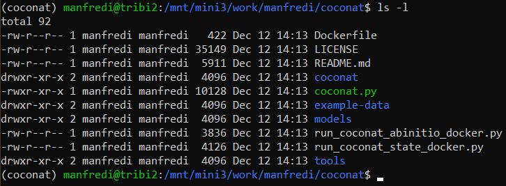
  Figure 4. Configuration of local installation. The screenshot displays the content of the CoCoNat folder after downloading the GitHub repository in a local folder. The word “coconat” between parenthesis at the beginning of the prompt (in white) appears only if the conda environment is properly set up.
2. Run CoCoNat (see Figure 5).
  1. Prepare your sequences in FASTA format. Input requirements are the same as the online predictions but without limits on the number and length of the sequences. Please remember that the maximal number of sequences and the maximal length of each sequence that the model will be able to process together will depend on the specifics of your machine.
  2. Run the run_coconat_abinitio_docker.py script, providing paths to the input FASTA file, the output TSV file, and the models downloaded at step C1e.
    
    cd coconat
    python run_coconat_abinitio_docker.py \
    --fasta_file=example-data/example.fasta \
    --output_file=example-data/example.tsv --plm_dir=${HOME}/coconat-plms
  3. (Optional) Run instead the run_coconat_state_docker.py script, providing an additional input file, to run predictions with precomputed coiled-coil segments. The input segment file must be a TSV containing a row for each precomputed segment and four columns:
    i. ID of the protein containing the segment.
    ii. Segment start.
    iii. Segment end.
    iv. Registers sequence of the segment.
    
    cd coconat
    python run_coconat_state_docker.py \
    --fasta_file=example-data/example.fasta \
    --seg_file=example-data/example-seg.tsv
    --output_file=example-data/example.tsv --plm_dir=${HOME}/coconat-plms
    
    See step A9a for a description of the output file generated by the program.
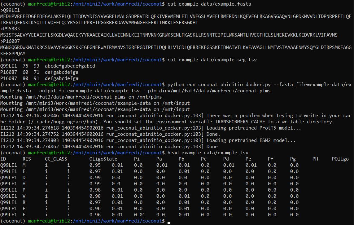
  Figure 5. Local execution. The screenshot displays the execution of an example contained in the GitHub repository. At the top, the content of the input files is displayed, including a FASTA file and a segment file. The third command is the execution of the CoCoNat script, followed by the expected messages given during a normal execution. Finally, the last command shows the first 10 lines of the output file in tab-separated format. The meaning of each column is detailed in step A9a.
3. For further help and details please reference the README provided in the GitHub repository (https://github.com/BolognaBiocomp/coconat).

Validation of protocol

This protocol or parts of it has been used and validated in the following research article(s):

Madeo et al. (2023). CoCoNat: a novel method based on deep learning for coiled-coil prediction. Bioinformatics (Tables 3, 4, 5).

Acknowledgments

The work was supported by the European Union—NextGenerationEU through the Italian Ministry of University and Research under the projects “Consolidation of the Italian Infrastructure for Omics Data and Bioinformatics” (ElixirxNextGenIT)” (Investment PNRR-M4C2-I3.1, Project IR_0000010, CUP B53C22001800006) and "HEAL ITALIA" (Investment PNRR-M4C2-I1.3, Project PE_00000019, CUP J33C22002920006).

This protocol describes the method presented in Madeo et al. (2023).

Competing interests

There are no conflicts of interest or competing interests.

References

Crick, F. H. C. (1952). Is α-Keratin a Coiled Coil? Nature 170(4334): 882–883. https://doi.org/10.1038/170882b0
Truebestein, L. and Leonard, T. A. (2016). Coiled-coils: The long and short of it. Bioessays 38(9): 903–916. https://doi.org/10.1002/bies.201600062
Walshaw, J. and Woolfson, D. N. (2001). Socket: a program for identifying and analysing coiled-coil motifs within protein structures. J. Mol. Biol. 307(5): 1427–1450. https://doi.org/10.1006/jmbi.2001.4545
Szczepaniak, K., Bukala, A., da Silva Neto, A. M., Ludwiczak, J. and Dunin-Horkawicz, S. (2021). A library of coiled-coil domains: from regular bundles to peculiar twists. Bioinformatics 36(22–23): 5368–5376. https://doi.org/10.1093/bioinformatics/btaa1041
Madeo, G., Savojardo, C., Manfredi, M., Martelli, P. L. and Casadio, R. (2023). CoCoNat: a novel method based on deep learning for coiled-coil prediction. Bioinformatics 39(8). https://doi.org/10.1093/bioinformatics/btad495
Elnaggar, A., Heinzinger, M., Dallago, C., Rihawi, G., Wang, Y., Jones, L., Gibbs, T., Feher, T., Angerer, C., Steinegger, M., et al. (2020). ProtTrans: Towards Cracking the Language of Life’s Code Through Self-Supervised Deep Learning and High Performance Computing. arXiv. Retrieved from http://arxiv.org/abs/2007.06225
Lin, Z., Akin, H., Rao, R., Hie, B., Zhu, Z., Lu, W., Smetanin, N., Verkuil, R., Kabeli, O., Shmueli, Y., et al. (2022). Evolutionary-scale prediction of atomic level protein structure with a language model. bioRxiv https://doi.org/10.1101/2022.07.20.500902
Feng, S.-H., Xia, C.-Q. and Shen, H.-B. (2022). CoCoPRED: coiled-coil protein structural feature prediction from amino acid sequence using deep neural networks. Bioinformatics 38(3): 720–729. https://doi.org/10.1093/bioinformatics/btab744
Tan, T., Tong, J., Khan, A. M., de Silva, M., Lim, K. and Ranganathan, S. (2010). Advancing standards for bioinformatics activities: persistence, reproducibility, disambiguation and Minimum Information About a Bioinformatics investigation (MIABi). BMC Genomics 11: S27. https://doi.org/10.1186/1471-2164-11-s4-s27

Supplementary information

The following supporting information can be downloaded here:

File S1.

Article Information

Copyright

How to cite

Manfredi, M., Savojardo, C., Martelli, P. L. and Casadio, R. (2024). CoCoNat: A Deep Learning–Based Tool for the Prediction of Coiled-coil Domains in Protein Sequences. Bio-protocol 14(4): e4935. DOI: 10.21769/BioProtoc.4935.

Download Citation in RIS Format