- Protocols

- Articles and Issues
- For Authors
- About
- Become a Reviewer

A Protocol to Retrieve and Curate Spatial and Climatic Data from Online Biodiversity Databases Using R
Published: Vol 13, Iss 20, Oct 20, 2023 DOI: 10.21769/BioProtoc.4847 Views: 1897
Reviewed by: Prashanth N SuravajhalaJeff W Bizzaro
Original research article
The authors used this protocol in:
Aug 2022
Advertisement


Protocol Collections
Comprehensive collections of detailed, peer-reviewed protocols focusing on specific topics


Abstract
Ecological and evolutionary studies often require high quality biodiversity data. This information is readily available through the many online databases that have compiled biodiversity data from herbaria, museums, and human observations. However, the process of preparing this information for analysis is complex and time consuming. In this study, we have developed a protocol in R language to process spatial data (download, merge, clean, and correct) and extract climatic data, using some genera of the ginseng family (Araliaceae) as an example. The protocol provides an automated way to process spatial and climatic data for numerous taxa independently and from multiple online databases. The script uses GBIF, BIEN, and WorldClim as the online data sources, but can be easily adapted to include other online databases. The script also uses genera as the sampling unit but provides a way to use species as the target. The cleaning process includes a filter to remove occurrences outside the natural range of the taxa, gardens, and other human environments, as well as erroneous locations and aspatial correction for misplaced occurrences (i.e., occurrences within a distance buffer from the coastal boundary). Additionally, each step of the protocol can be run independently. Thus, the protocol can begin with data cleaning, if the database has already been compiled, or with climatic data extraction, if the database has already been parsed. Each line of the R script is commented so that it can also be run by users with little knowledge of R.
Keywords: EcologyBackground
Our knowledge of species distributions is central to biogeographers but also to phylogeneticists and ecologists. Indeed, species distributions are needed to perform phylogenetic climate reconstructions, species niche characterizations, or species distribution models, and to address many evolutionary questions. However, obtaining accurate spatial information on species distributions requires occurrence databases of good quality, with high geographical coverage, which are difficult to obtain.
The main sources of geographical information are field inventories and biodiversity collections (museums and herbaria), for which accessibility has been a serious limitation until recently. The digitization efforts of recent decades have facilitated access to vast amounts of biodiversity data previously scattered in different institutions around the world, through online databases such as the Global Biodiversity Information Facility (GBIF; GBIF.org, 2021). As a result, we now have an unprecedented opportunity to benefit from centuries worth of naturalist observations from all over the world. However, the use of this valuable information is limited by persistent knowledge gaps and technical limitations. On the one hand, our knowledge of species distributions is still poor, biased, or imprecise (Hortal et al., 2007), and this is reflected in the information collected in biodiversity databases, which is not consistent across lineages or across regions. These biases result in some groups of organisms and regions of the world having scarce information while others have large amounts of data (Hortal and Lobo, 2005). On the other hand, the complexity of the process of parsing and preparing online data for analysis is high. For example, it is common for online repositories to contain records with imprecise or erroneous spatial information (such as terrestrial organisms with records in the sea) or with outdated taxonomic nomenclature (Soberón and Peterson, 2004). Therefore, every study based on online data requires a first step of cleaning and parsing to remove or minimize the impact of these sources of uncertainty (persistent knowledge gaps and technical limitations) on further analysis (Hortal et al., 2007).
In parallel with the international digitization efforts of the last decades, several methods and pipelines have been designed to deal with these sources of uncertainty and to simplify the different steps of working with online biodiversity data. Some of the most relevant protocols have been developed in R (R Core Team, 2018) and include geographic, taxonomic, or temporal data cleaning (see for example: Biogeo, Robertson et al., 2016; SpeciesGeoCorder, Töpel et al., 2016; CoordinateCleaner, Zizka et al., 2019; bRacatus, Arlé et al., 2021; BDcleaner, Jin and Yang, 2020; plantR, Lima et al., 2021). However, none of them address the uncertainty introduced by both the spatial knowledge gaps and the technical limitations. Moreover, most of them focus on one or a few steps of the process. Thus, to complete the process (from the initial download of occurrences to the climatic data extraction of the cleaned and parsed spatial database) users have to deal with different protocols, some of which require programming skills or a deep R background.
The R protocol that we present here is designed to produce reliable databases of species occurrences and climate data from online repositories. It provides an automatic procedure for dealing with the most common sources of spatial uncertainty in online biodiversity databases. It also includes an automatic script to run each sample (species, genus, family, etc.) separately, allowing for an easy and fast way to process hierarchical databases. The script also includes a post-processing code to run after the spatial pipeline and extract the climatic data. The protocol describes a step-by-step guide on how to download, parse, clean, and merge spatial and climatic data from three online databases (Figure 1; WorldClim, Fick and Hijmans, 2017; BIEN, Maitner, 2020; GBIF, GBIF.org, 2021). Moreover, the protocol can be easily adapted to include any other online biodiversity database that may be of interest. The cleaning steps include how to automatically update nomenclatural information, identify, and remove records outside the natural distribution of taxa, records from gardens and other human environments, or geographically inaccurate records. To explain the protocol, we used the AsianPalmate Group (AsPG) of Araliaceae as a case study, using genera as a sample unit. To speed up the implementation, we selected 16 of the AsPG genera. The selection of genera was made to exhibit uneven spatial information across genera and across areas of the world. This approach aimed to address the issue derived from knowledge gaps as a source of spatial uncertainty. Additionally, the chosen genera are largely affected by erroneous and misplaced records, serving to tackle the issue arising from technical limitations as a source of spatial uncertainty.
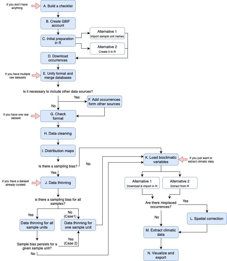
Figure 1. Workflow for the entire protocol pipeline. It includes all the steps and alternatives described in the protocol. Each red arrow represents the steps of the protocol that we can start with, depending on the data available.
In summary, the main advantages of this protocol are that it: (1) can be applied to all groups of organisms (as long as they have information available in GBIF or BIEN databases) and at any taxonomic rank, not only at the species level; (2) provides an automatic way to handle hierarchical databases, which is very helpful when studying highly diversified groups (genera with a high number of species, families with a high number of genera, etc.); (3) provides a complete pipeline from spatial data download (including merging multiple databases) to climatic data extraction; (4) deals with uncertainties arising from technical limitations (such as incorrect records), but also with the uncertainties arising from persistent knowledge gaps (such as spatial biases in different parts of the world and across lineages); (5) provides an easy way to filter out records outside the natural range of the taxa; (6) applies a spatial correction for erroneous occurrences outside the coastal boundary; (7) includes independent steps for each part of the process that can be run separately; and (8) can be easily used and modified by any types of users regardless of their skills, knowledge, or background on R, because it is accompanied by instructions to guide the user.
Equipment
Computer with Microsoft® Windows® 10 education, KUBUNTU 22.04, or Mac® OS X® 12.6 operating systems and versions.
Software
R version 4.3.1 (https://r-project.org/)
Packages: "BIEN", "countrycode", "data.table", "devtools", "dpyr", "plyr", "raster", "readr", "rgbif", "rgdal", "spocc", "spThin", "SEEG-Oxford/seegSDM" and "tidyr".
RStudio version 2023.06.0+421 (https://rstudio.com/products/rstudio/)
The use of RStudio is optional. RStudio is an interface that improves the use of R.
Databases
POWO (https://powo.science.kew.org)
GBIF (https://www.gbif.org/)
WorldClim (https://www.worldclim.org/)
Procedure
The R script can be freely downloaded from GitHub (https://github.com/NiDEvA/R-protocols; Note 1). The pipeline of the procedure coincides with the steps of the R script of this protocol (Figure 1). First, you need to create two working folders, one called “input” (it contains the information needed to run the R script) and another one called "output" (it will contain the resulting files after running the R script). In this protocol, we used the genus rank as the operational taxonomic unit, but the script also contains commented lines (those preceded with "#") with the functions needed if you want to use species as the sample unit. Besides, it can also be easily modified to use family or any other higher taxonomic level as the operational unit if needed. We have also cleaned the data by removing records outside the natural distribution of genera, from gardens and other human environments, or those that are geographically inaccurate, but it can also be readily adjusted to meet specific data cleaning requirements as needed.
Prepare a checklist of the native range of the taxa
It is necessary to know the countries where the taxa are native. For plants, this information can be found in the World Checklist of Selected Plant Families (WCSP, Govaerts et al., 2008). WCSP is a database that compiles checklists of 200 seed plant families, and it is available in Plants of the World Online (POWO, 2023; http://www.plantsoftheworldonline.org/). The database is frequently updated, and each new name published in the International Plant Name Index (IPNI; International Plant Names Index, 2020) is reviewed and added to POWO. Other sources of information on the natural range of other organisms are available in ASM Mammal Diversity Database (https://www.mammaldiversity.org/index.html, Mammal Diversity Database, 2020), Avibase - The World Bird Database (https://avibase.bsc-eoc.org/avibase.jsp, Lepage et al., 2014), Catalogue of Life ( https://www.catalogueoflife.org/, Bánki et al., 2022), Checklist of Ferns and Lycophytes of the World (Hassler, 2022a), Global Assessment of Reptile Distributions (http://www.gardinitiative.org/, GARD, 2022), Reptile Database (http://www.reptile-database.org/, Uetz et al., 2021), USDA Plants Database (https://plants.usda.gov, USDA, NRCS, 2022), and World Plants (https://www.worldplants.de , Hassler, 2022b). For plants not included in POWO or for animals, go to steps A1–A4 to manually create the list of countries where the taxa are native. For plants included in POWO database, go to step A5 to automatically create the list of native countries.
Create a text file in a text editor (e.g., Notepad++, BBedit, or Notepadqq in Linux), with the names of all taxa separated by "Enter" in a plain text editor. Save it as "Natural_Distribution_Checklist_TDWG.txt".
Go to https://wcsp.science.kew.org/home.do (or the corresponding webpage, see above) and enter the taxon name in the search engine. WCSP uses two ways to describe the distribution of taxa, one in narrative form and the other one through international codes (Figure 2). The international code used in WCSP is the third level of geographical codes of the Taxonomic Databases Working Group (TDWG, Brummitt, 2001) (Note 2).
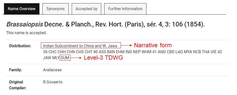
Figure 2. Example of Brassaiopsis genus in WCSP. WCSP provides status, distribution, family, and original compiler information of each taxon.Copy each code of three capital letters (just the codes, not the numbers that appear at the beginning of the country code line) and paste in "Natural_Distribution_Checklist_TDWG.txt" in the same line right after the corresponding taxa name separated by ";". In some cases, symbols ["?", "(?)", "+", "†"] or lowercase letters may appear in distribution. According to TDWG, "?" is used when the presence of a taxon in a given area is not certain. If this symbol is used within brackets, it is because there is no exact location known within a country. When a taxon is extinct or may be extinct in an area, the symbol "†" is placed after the country code. When the country code is not known, "+" is used. Lowercase letters for the country code indicate naturalization. For this protocol, we have only used the codes with three capital letters that do not have any symbols. For more information, consult the "about checklist" section on the WCSP website.
Repeat steps A2 and A3 until all taxa are completed and save the document in the "input" folder. The format of the resulting text file should look as in Figure 3. It is advisable to sort the taxa alphabetically in the text file.
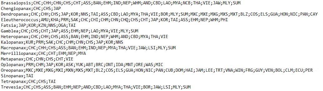
Figure 3. Format for the text file containing the natural distribution countries of the taxa. The first element of each row is the name of an AsPG genus followed by the Level-3 TDWG code of the countries where the taxa occur naturally, separated by a semicolon.Additionally, steps A1–A4 can be automated in R for plants included in POWO. We have provided a working example in the code (see point 5 in the code). However, it is important to note that many families are not included in the POWO database, so in most cases it will be necessary to generate the list manually as indicated in steps A1–A4.
Create an account in GBIF database
Visit the website https://www.gbif.org/. Click on Login located in the upper-right corner of the website, and then on REGISTER (Figure 4).

Figure 4. Home of the GBIF Database. To create an account, it is necessary to fill the required information in the section Register; remember the information included, because it will be necessary later in the R protocol.Fill the COUNTRY, EMAIL, USERNAME, and PASSWORD fields, click on next, and follow the instructions to create the account. It is also possible to create the account through Google, Facebook, or GitHub. Important to remember: save the information filled in the email, username, and password, because it will be used later in the R script.
Initial preparation in R
Open RStudio (Note 3).
Create the paths in R for the input and output data. These paths correspond to the "input" and "output" folders. Replace the example path with the path of the “input” folder.
Install and load the packages needed to run the R script. This packages are "BIEN" (Maitner et al., 2018), "countrycode" (Arel-Bundock et al., 2018), "data.table" (Dowle et al., 2019), "devtools" (Wickham et al., 2021), "dplyr" (Wickham et al., 2020), "plyr" (Wickham, 2020), "raster" (Hijmans et al., 2020), "readr" (Wickham et al., 2018), "rgbif" (Chamberlain et al., 2020a), "rgdal" (Bivand et al., 2020), "seegSDM" (Golding and Shearer, 2021), "spocc" (Chamberlain et al., 2020b), "spThin" (Aiello-Lammens et al., 2019), and "tidyr" (Wickham et al., 2022). The packages can be downloaded directly into RStudio with the "install.packages" function, except for the "seegSDM" package, which is installed through the "devtools" package as it is specified in L63 of the R script. In this protocol we use BIEN (https://www.biendata.org/) and GBIF (https://www.gbif.org/) as the online biodiversity databases for obtaining the spatial data; if you want to include any other online database to obtain records for your case study, you will need to look for the correspondent R package and install them at this step of the protocol.
Create a vector with the names of the taxa (sample unit). The vector can be created in R (see "Alternative 1" in the R script) or it can be imported from a file (.csv, .txt, .xls; see "Alternative 2" in the R script). For this protocol, we read the file on the GitHub page “Alternative 3”, as we already have the information in GitHub for this example. Be aware that the names and order of sample units must be exactly the same as in the "Natural_Distribution_Checklist_TDWG.txt" file (see above step A1).
Read the natural distribution text file built in procedure A named "Natural_Distribution_Checklist_TDWG.txt". First, load in R the text file that contains the natural distribution of sample units as a vector. Then, convert the vector into a list. Each item in the list corresponds to a genus (or the correspondent sample unit: species, family, etc.) followed by its corresponding Level-3 TDWG country codes, separated by ";".
Download the occurrence data from online databases (GBIF and BIEN, or the desired database)
Use the package "rgbif" to download the records from the GBIF database.
Indicate the username, email, and password created in step B2. Replace the "XX" with your credentials (important to not remove the "characters").
Search the taxon keys of each taxon. GBIF has a key to identify each taxon in the database. In case you use species or families instead of genera as the sample unit, replace rank = "genus" in the name_backbone function with rank = "species" or rank = "family", respectively.
Prepare the download request and download data.
i. Create the path to a folder that will contain the files downloaded from GBIF and create a folder inside the "input" folder, naming it as "download_GBIF". This folder will contain the files downloaded from GBIF. Indicate the number of taxa included in the text file with the checklist of taxa native range.
ii. Prepare and download the occurrences. The download request is executed with the "occ_download" function, which allows you to establish criteria for filtering the data downloaded. In this protocol, as we wanted to keep only native records with coordinates, we used the arguments explained in Table 1. The "occ_download_wait" function indicates the status of the download, and the code continues running until the status changes to “succeeded”. The download is performed with the "occ_download_get" function and will result in as many zip files inside the "download_GBIF" folder as taxa included in your request. The "occ_download_import" function imports into R the data set downloaded from the "download_GBIF" folder (Note 4).
Table 1. Necessary arguments of the occ_download function from “rgbif” package
Argument Description To download pred Downloads only the occurrences equal to unique condition Select "taxon" for "taxonKey" and TRUE for "hasCoordinate" pred_not Downloads only the occurrences not equal to the condition Select "INTRODUCED", "INVASIVE", "MANAGED", and "NATURALISED" for "establishmentMeans" pred_in Downloads the occurrences equal to multiple conditions Select "taxon.keys" for "taxonKey"
Use the BIEN_occurrence_genus function from R package "BIEN" to download the records from the BIEN database version 4.1.1 (Note 5). It is necessary to indicate some arguments to start the download (Table 2). We will refer to the resulting data set as “raw.BIEN.dataset” onwards. If there are no records in “raw.BIEN.dataset”, go directly to step E3 to replace the column names and see Note 6.
Table 2. Necessary arguments of the BIEN_occurrence_genus function from “BIEN” package. If you use species as the sample unit, then you will need to use the BIEN_occurrence_species function; replace the argument "genus" with "species" with the remaining arguments staying the same.
Argument Description For download genus Name of genus This argument corresponds to the vector of taxa names created in R (taxa.names) cultivated If TRUE, it also returns cultivated occurrences Select FALSE (it is selected by default) all.taxonomy If TRUE, it returns all taxonomic information Select TRUE (FALSE is selected by default) collection.info If TRUE, it returns additional information about collection and identification Select TRUE (FALSE is selected by default) observation.type If TRUE, it returns information on type of observation Select TRUE (FALSE is selected by default) political.boundaries If TRUE, it returns information on political boundaries Select TRUE (FALSE is selected by default) natives.only If TRUE, it returns only native species Select TRUE (is selected by default) Save the R workspace with the downloaded data as "1_Workspace_Download.RData". It is very useful to save the objects created in the downloaded data. If there is a problem in later steps, this workspace can be loaded and thus avoid making another download.
Unify the format of the downloaded databases and simplify the database by removing unnecessary columns
In order to join the information from the two databases, the number of columns and their names have to be identical in "raw.GBIF.list" and "raw.BIEN.dataset". Note that some columns from GBIF and BIEN have different names and yet contain the same information. In those cases, it is necessary to rename the columns (see below). Columns with information that will not be used in further analysis can be removed in this step too.
Simplify raw GBIF data set "raw.GBIF.list".
Create new columns for future merging between GBIF and BIEN raw data sets.
i. Add the "countryName" column to include full country names using the "countrycode" R package and the "countryCode" column. The "countryCode" column includes a 2-letter ISO 3166-1 standard for country codes and their subdivisions. This standard is used by GBIF to indicate the country in which the occurrence was recorded, while BIEN uses the full name. The “countrycode” function transforms the "countryCode" column in country names (Note 7).
ii. Add “dataOrigin” column filled with GBIF. This column indicates if the record belongs to GBIF or BIEN; in this case, it will be filled with “GBIF” for all records.
Select useful columns to simplify the data set before merging with BIEN. The number of columns of "raw.dataset" is approximately 50; it is advisable to reduce this number. For our purpose, the useful information is inside the following columns: "gbifID", "dataOrigin", "basisOfRecord", "genus", "species", "scientificName", "decimalLongitude", "decimalLatitude", "elevation", "countryName", "countryCode", "locality", "eventDate", "institutionCode", "collectionCode", and "catalogNumber". Therefore, we will keep only these columns. We will refer to the resulting data set as "simple.GBIF.dataset" onwards.
Export "simple.GBIF.dataset" as a csv file.
Simplify raw BIEN data set "raw.BIEN.dataset".
Remove duplicated columns. In the download, the "data_collected" column is duplicated. This is because the "collection.info=TRUE" argument in the download adds the column "data_collected" in addition to other variables. However, if we select "collection.info=FALSE", we would lose other variables related to collection information and, thus, it is necessary to use “TRUE” (Note 8).
Remove records that are also from the GBIF database to avoid replicated data. BIEN data source may contain occurrences that are also in GBIF, this information is available in the "datasource" column of "raw.BIEN.dataset".
Create necessary columns for merging with GBIF. Add the country code and elevation variables.
i. Add the country codes assigned by the 2-letter ISO 3166-1 standard from the name of the country available in "country" column of “simple.BIEN.dataset”.
ii. Add an empty elevation column with "NA" (Not Available information). The elevation is not included in the downloaded information from BIEN, but it is included in GBIF, and we do not want to lose this information when merging the two databases.
iii. Add an empty "ID_Origin" column filled with "NA". This information is not available in the BIEN database, but it is included in GBIF, and we do not want to lose this information.
iv. Add "dataOrigin" column filled with BIEN. This column indicates if the record belongs to GBIF or BIEN; in this case, it will be filled with BIEN for all records.
v. If your sample unit is species and you have used "BIEN_occurrence_species" to download the data, then you will not have any column indicating the name of the genus. Since this column may be of interest, then it is desirable to run this function to add a column with the name of the genera, named "scrubbed_genus". This line is commented on the script and, thus, it is not performed in the protocol unless you uncomment it (Note 9).
Select useful columns from all available variables. For our purpose, the useful information is inside the following columns: "ID_Origin", "dataOrigin", "observation_type", "scrubbed_genus", "scrubbed_species_binomial", "verbatim_scientific_name", "longitude", "latitude", "country", "country_ISOcode", "locality", "date_collected", "datasource", "collection_code", and "catalog_number". Therefore, we will keep only these columns. We will refer to the resulting data set as "simple.BIEN.dataset" onwards. Note that the R object "ID_Origin" contains the code of the record in the original database but transformed as exponential. To look for the exact original code, go to that field in the exported ".csv".
Export "simple.BIEN.dataset" as a csv file.
Match columns between "simple.GBIF.dataset" and "simple.BIEN.dataset". To merge the two data sets you need to rename columns in both objects to match the following extract names ("ID_Originin", "Data_Origin", "Basis_of_Record", "Genus", "Spp", "Scientific_name", "Longitude", "Latitude", "Elevation", "Country_Name", "Country_ISOcode", "Locality", "Date", "Institution_code", "Collection_code", and "Catalog_number") and following the equivalences indicated in Table 3. If there are no records in “raw.BIEN.dataset”, it is important that you see Note 10.
Table 3. Equivalences between information of GBIF and BIEN simple data sets needed for merging data sets. Names of selected columns of "simple.GBIF.dataset" and "simple.BIEN.dataset", and their corresponding name in the merged data set.
GBIF BIEN Merged ID_Originin (new) ID_Originin ID_Originin Data_Origin (new) Data_Origin Data_Origin genus scrubbed_genus Genus species scrubbed_species_binomial Spp scientificName verbatim_scientific_name Scientific_name decimalLatitude latitude Longitude decimalLongitude longitude Latitude elevation Not available (Later created as "elevation") Elevation countryName (new) country Country_Name countryCode Not available (Later created as "country_code") Country_code locality locality Locality eventDate date_collected Date institutionCode datasource Institution_code collectionCode collection_code Collection_code catalogNumber catalog_number Catalog_number basisOfRecord observation_type Basis_of_Record Merge "simple.GBIF.dataset" and "simple.BIEN.dataset". Build the new data set from the equivalence information of the "simple.GBIF.dataset" and "simple.BIEN.dataset" objects specified in Table 3. The resulting table has the information of both data sets, and it has 16 variables. We will refer to the resulting data set as "merged dataset" onwards. If there were no records in "raw.BIEN.dataset", you still need to rename your "simple.GBIF.dataset" to "merged.dataset", because it is the name used onwards in the R script (Note 10).
Save "merged.dataset" as a csv file named "2_merged_dataset.csv". This file contains all the simplified GBIF and BIEN information. Or only GBIF data, in case no record was downloaded from BIEN.
Add occurrences from other sources
This procedure is only necessary if the data from GBIF and BIEN is incomplete (that is, they do not completely reflect the distribution range of the study case) and the author deems it necessary to include other data sources (such as additional online databases, herbarium specimens, or citations in the literature) to complete taxa ranges. If this is not the case, skip this procedure and go to G.
For additional online databases. In this protocol, we will use only GBIF and BIEN occurrences downloaded using "rgbif" and "BIEN" R packages. This step is commented on the R script. However, we provide an optional example using package "spooc" in R. This package can download occurrences from a diverse set of data sources, including Global Biodiversity Information Facility (GBIF; GBIF.org, 2021), USGS Biodiversity Information Serving Our Nation (BISON, 2021), iNaturalist (2021), Berkeley Ecoinformatics Engine (2021), eBird (Sullivan et al., 2009), Integrated Digitized Biocollections (iDigBio, 2021), VertNet (2021), Ocean Biogeographic Information System (OBIS; Grassle, 2000), and Atlas of Living Australia (ALA, 2021). The procedure with this package is very similar to the one already done in this protocol with BIEN and GBIF. The result of the download is a list with as many elements as taxa in the "taxa.names" vector. Each of these elements contains information on the given taxon in the eight databases. Once the "spooc" R package has been run, you will need to reformat and simplify the downloaded databases so that they match the column names and structure specified in step E3. To do this, first go to step E2b and adapt the script onwards to remove GBIF replicates (E2b), create a match column to merge the databases (E2c), adapt the script in E2d to identify the columns of interest, and in E2e export the results in a file named "simple.spooc.dataset". Then adapt E3 to rename columns in "simple.spooc.dataset" as already done for GBIF and BIEN. Finally, go to E4 and adapt it to merge the three databases ("simple.spooc.dataset", "simple.GBIF.dataset", and "simple.BIEN.dataset").
For georeferenced herbarium specimens and literature occurrences. The exported csv file "merged_dataset.csv" is used to manually add the records obtained from herbaria and literature.
Open Microsoft Excel.
Import "merged dataset" csv file exported in step E5.
i. Select "Data > Get External Data > From text" and open de "merged_dataset.csv" file. A new window, called "Text Import Wizard", will appear.
ii. Select "Delimited" in "Original Data Type" and click on "Next".
iii. Select "Comma" in "Delimiters" and click on "Next".
iv. It is advisable to select "Text" in "Column data format" for all columns of the file. Click on "Next". This is done to avoid problems with cell format in Excel that occur in columns that have special characters and symbols and, also (and most importantly), in the columns that include the coordinates.
Add new occurrences filling all the fields of the variables of the table. When no information is available, complete the field with NA. This format will make the importation of the database to R easier (Note 11).
Export the table as csv.
i. Select "File > Save as".
ii. A new window will appear. Choose the "input" folder as the destination folder for the file. Introduce "merged_dataset_Version2" as the file name and select "CSV (Comma delimited) (*.csv)" as the file type. Click on "Save". If you are using Excel for MacOS, then export as "MS-DOS Comma Separated (.csv)" and check that the separators are commas. If that is the case, then run line 260. If separators are semicolons, run the line 259 in R script.
iii. A new window will appear to remind you that only the active spreadsheet will be saved. Select "OK". Select "OK" in the next window that appears.
Check the “merged.dataset” object
It is necessary to check that the data set has the correct format.
If you come from step F2, return to RStudio and import the csv file obtained in step F2diii, "merged_dataset_Version2.csv". This step is commented in the R script because it has not been done in this protocol. If you come from procedure E or step F1, go straight to step G2.
Visualize "merged.dataset". Check that the number of columns in the data set is 16. The structure must be a data.frame. "Latitude", "Longitude", and "Elevation" must be in numeric format, and the rest of the columns must be in character format (Note 12).
Data cleaning
This procedure is focused on cleaning the most common errors.
Remove the records that lack decimal coordinates. This was already done for GBIF records during the import in step D1 but is necessary for records imported from the BIEN database (or any other database if you run F1, Note 12).
Remove the records with invalid coordinate values (that is, Longitude or Latitude = 0). This is common in records from GBIF.
Remove the records in which coordinates have low precision (for the geographical scale and our purposes, we have removed the coordinates that had less than 1 decimals, this can be modified in the script to meet the precision you need as indicated in the R script).
Remove replicated records among databases. Delete the rows that have the same information for the fields: "Genus", "Spp", "Date", "Locality", "Longitude", "Latitude", "Elevation", "basisOfRecord", "catalogNumber", and "CountryCode". Sometimes, the same record has been uploaded in different databases; avoiding redundant data is desirable to reduce processing time. Note that this filter is tied to the number of decimals.
Remove records outside natural distribution of the taxa. Each record of the database after running steps H1–H4 (that is, R object “filtered.dataset”) is compared with a filtered version ("checklist.filtered") of the checklist obtained in step A5 ("checklist"), and those outside the natural distribution will be removed.
Add level-3 TDWG code to "filtered data" for future comparison with the checklist created in step A4.
i. Load the world shapefile with the level-3 TDWG code used by WCSP available in GitHub https://github.com/tdwg/wgsrpd.
ii. Select the WGS84 projection to the shapefile using the "crs" function from "raster" package.
iii. Extract level-3 TDWG code for the occurrences from "filtered.data" (Note 13).
iv. Remove records outside the limits of the level-3 TDWG shapefile. These records correspond to the ones that have "NA" values in the "LEVEL3_COD" column and, also, to those in which coordinates place the occurrence in the sea (because our study case is terrestrial). Remove the "optional" column that is created by default when using the "extract" function (Note 14).
Divide your data set ("filtered.data.TDWG") in sections according to your sample unit. Each section is a table with the records of one genus. Be aware that the sections of this table must correspond to the sample unit of your study (family, genus, species, etc.). Check that the taxa names appearing in "Name" column of the "checklist.filtered" that is cleaned in line 445 of the R script are the same as those indicated at the beginning of the "value" column of the same object.
Filter your data set ("filtered.data.TDWG") to retain only natural records. Compare each genus (or the correspondent sample unit) with the countries of its natural distribution. The "Country_TDWGcode" column of a given sample unit is compared with the corresponding element of "filtered.checklist" created in step H5b from the original checklist created in step A5. The resulting object is a list that contains all the filtered occurrences, and that is converted into a dataframe (“filtered.dataset.WCSP” onwards). Although GBIF database has a column that indicates if the record comes from cultivation, it is highly advisable to run this part of the script to remove naturalized records as well.
Export the "filtered.dataset.WCSP" object as "3_Cleaning_dataset_WCSP.csv" and save the workspace as "2_Workspace_Cleaning.RData".
Distribution maps
This procedure is focused on visualizing the global distribution of all taxa together and individual maps of each sample unit after data cleaning.
Create a global distribution map with all sample units as a PDF named "4_global_distribution_map.pdf". The occurrences of all sample units are colored in red and the surface of the world in grey.
Create distribution maps for each sample unit as a PDF named "4_distribution_maps.pdf". Convert "filtered.dataset.WCSP" dataframe into a list in which each element of the list belongs to the occurrences of a single sample unit. Each page of the PDF contains a map of each sample unit (expanding the geographic area in which it appears) titled with the name of the taxon. The occurrences of each sample unit are colored in red and the surface of the world in grey.
Data thinning
The “spThin” package chooses an occurrence and removes nearby occurrences according to the indicated distance in the buffer. This procedure is intended to remove the bias when spatial data is unevenly distributed across your data set, and there are certain areas for all or a few sample units that are disproportionately sampled. To identify this sampling bias, visually inspect the maps created in procedure I. If your sampling bias affects most or all of your sample units, then proceed with the thinning in step J1a; if the sampling bias affects only one or two sample units, then proceed with the thinning in step J1b. If you detect sampling bias, the thinning is crucial to minimize errors in further spatial-based analyses, such as avoiding overestimation in the bioclimatic data and oversampled areas. If there is no bias in your data set, then you can skip this procedure and go to procedure K.
Remove occurrences randomly with a given distance buffer (50 kilometers in this case) from the "Latitude" and "Longitude" columns. You may need to modify this buffer based on the geographical scale of your case study. This is done in the "thin.par" argument of the "thin" function in the R script. It is very important to put the distance in kilometers. The random elimination of occurrences is done by sample unit. In our case study, the sample unit is indicated in the "Genus" column, but you can modify it in the script if needed.
Perform this step if you want to apply the thinning to all your sample units. The output of this step is a csv file for each sample unit that will be directly exported to the chosen directory (Note 15). If you want to apply the thinning to just one sample unit, then go to step J1b.
Perform this step if you want to run the thinning just in one sample. In this step you will only apply the thinning to the sample unit that is affected by sampling bias. If you have not run step J1a, then select the proper buffer based on your geographical scale (Case 1). If you perform this step because a given sample unit is still affected by sampling bias after running step J1a, you must increase the buffer with respect to the one used in step J1a (Case 2). This step has not been done in the protocol, but the procedure is included and commented on the R script (Note 16).
Import csv files after data thinning using R package "readr" from "thin" folder.
Import csv files for all the taxa obtained in step J1 if you only performed J1a or if you performed J1a and J1b (Note 17). Continue with step J3a.
Perform this step only if the thinning has been performed on only one sample unit (that is, if you run step I1b directly without running step I1a). Import csv file obtained in I1b for the sample unit thinned. This step is commented on the R script because it has not been done in this protocol. Continue with step I3b.
After data thinning, the exported files have only three columns: "Genus", "Longitude", and "Latitude". Therefore, if you run procedure I, add all the remaining 13 columns that contain the additional information of each record from the "filtered.dataset.WCSP" object to the data set obtained after the thinning ("thin.occ", in case you run step I2a; or "thin.taxon", in case you run step I2b).
If you come from step I2a, join columns of the "filtered.dataset.WCSP" to all thinned taxa imported in. Check that "thin.occ" has the same number of rows as "joined.dataset" (Note 18). Check that "joined.dataset" contains all the columns in "filtered.dataset.WCSP".
If you come from step I2b, join columns of the "filtered.dataset.WCSP" to one thinned taxon and add to the rest of the taxa of the "filtered.dataset.WCSP" object. This step is commented on the R script because it has not been done in this protocol (Note 18).
Export the joined file "joined.dataset" as a csv named "5_joined_dataset.csv" and save the workspace with thinned files as "3_Workspace_Thinning.RData".
Load bioclimatic variables from WorldClim version 2
This online climatic database contains 19 variables with the average values of 19 parameters that represent precipitation and temperature for the years between 1970 and 2000. There are two ways to obtain these bioclimatic variables. Alternative 1 is shown in step J1a, and it is available for all the resolutions available in WorldClim (10, 5, 2.5 min, and 30 s). Alternative 2 is shown in step J1b, and it is only available for resolutions of 10, 5, and 2.5 min.
Alternative 1. Download from the WorldClim website and import in R. We use the 30 s resolution, (only available on the website) because it is the highest resolution available and matches the minimum threshold for coordinate precision set in step H3 (two decimals in our case study). For this protocol, we used Alternative 2. If you use Alternative 1, uncomment lines in R code.
Go to the following link: https://www.worldclim.org/data/worldclim21.html. Click in bio 30s, unzip the zip file downloaded named "wc2.1_30s_bio.zip" (Figure 5), and rename the folder as "Bioclimatic _variables_WC2". Relocate this folder inside the "input" folder.
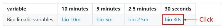
Figure 5. Download bioclimatic variables on the WorldClim websiteTo avoid sorting problems in R, rename bioclimatic variables as follows: replace original names ("wc2.1_30s_bio_1.tif") by adding a zero before the number or variable ("wc2.1_30s_bio_01.tif"). This is only done for variables 1 to 9.
Import bioclimatic variables to R. Remove "_" and ".tif" characters in column names.
Alternative 2. Download the standard WorldClim Bioclimatic variables directly from R using R package "raster". This alternative is only for the resolution of 10, 5, and 2.5 min. In the argument "res" of "getData" function, indicate 10, 5, or 2.5 for the resolution selected. Thus, if you chose for a minimum threshold of two decimals in step H3 and select this alternative, be aware that you will be losing precision for your climatic analysis. For this protocol, we used this alternative.
Spatial correction for terrestrial organisms
Despite the removal of all occurrences with inaccurate coordinates, it may happen that some of the occurrences may fall outside the limits of the earth's surface according to the limit of the cartographic base used as template. For terrestrial organisms, these occurrences may be wrong (if the distance to the coastal limit is huge) or simply misplaced (if the distance to the coastal limit is small). Because our ultimate goal is to extract climatic data (see procedure L), we do not want to include wrong occurrences, but it is desirable that we do not lose misplaced records. Thus, we need to check for occurrences out of the Earth’s limit to remove wrong occurrences and apply a spatial correction for misplaced occurrences. If there are no occurrences outside Earth’s limits in your database, go to procedure M and proceed with climatic data extraction. If there are occurrences outside the limits, then identify the occurrences that are between the coastal limit and 5 km from the coastal limit (misplaced occurrences) as established by bioclimatic variable 1 of WorldClim version 2 (same limit for the 19 available bioclimatic variables) and recalculate new coordinates so that the occurrence falls in the nearest climatic cell of the template. Occurrences located more than 5 km from the coastal limit (wrong occurrences) are eliminated (Note 19).
Visualize the distribution of all the filtered occurrences of the case study available in the "joined.dataset" object, using bioclimatic variable 1 as template. The map will be automatically exported to a PDF file. If you have not performed the thinning process in procedure J, uncomment the line 563 of the R script only.
Convert "joined.dataset" into the spatial object "joined.dataset.spatial".
Check if all "joined.dataset.spatial" points are within the boundaries of the bioclimatic variable layer. Occurrences located outside the layer boundaries are shown in red, located in the "outside_pts" object. The maps will be exported in a PDF file. If there are no occurrences in red, go to step M1 (Note 20).
Coordinate correction. Extract climatic data from bioclimatic variable 1 for all occurrences of the case study and identify which points have no climatic data (NAs, Note 19). The "nearestLand" function of the "seegSDM" package recalculates the coordinates of the occurrences that lie between the distance set in "dist" and the coastal limit to place it in the nearest climatic cell, and thus obtain climatic data. To check coordinate correction, maps with corrected points in green and uncorrected points in red appear in the viewer in the lower right corner of the RStudio screen. The process is repeated by increasing the distance by 1 km until a 5 km distance from the coastal limit is reached. Occurrences outside the 5 km are removed.
Extract climatic data from bioclimatic variable layers
Convert “joined.dataset” to spatial object and select WGS84 projection (Note 20).
Extract bioclimatic data. We use the "bilinear" method because this method returns values that are interpolated from the values of the four nearest raster cells. The "simple" method returns values in which the point falls. Using the "bilinear" method, we assume that the coordinates of the data set have a certain precision error, whereas if we use the “simple” method this error is ignored. Be aware that this step can be time consuming (Note 21).
Join the bioclimatic values to "joined.dataset" in a new dataframe named "climatic.data" and remove "optional" column created during the extraction of climatic data.
Visualize and export the final data set as “6_Final_dataset.csv”
Save the final workspace as "4_Workspace_Final_Data.RData".
Notes
Any text line preceded by the character "#" in the R script available from GitHub ("commented lines") is only intended to guide the user or to provide alternative code to run under specific cases and will not be run when executed in the R console. If the specific case applies to you, and you need to run the functions in the commented line, you need to uncomment the line (remove "#") and execute it. To comment on a section of R script press "Ctrl + Shift + C", and it will not run.
In case the WCSP geographical information for a given taxon is incomplete or not available, complete the natural distribution of the sample unit in other sources such as literature or other checklists and include it in the text file using the level-3 TDWG code (available in Brummitt, 2001), as mentioned in steps A3 and A4.
To run the lines of the script in RStudio, place the mouse cursor at the beginning of the line or selected regions of the code and press "Ctrl + Enter". If the line is uncommented (that is, not preceded by "#"), it will be run.
Check in the "download_GBIF" folder that there is a zip file with the reference of the "gbif.download.key" object. The results are also available on your downloads user page of GBIF: https://www.gbif.org/user/download.
Replace the function "BIEN_occurrence_genus" with "BIEN_occurrence_species" when sample unit is species and the argument "genus" by "species" inside the function.
If there are no records in "raw.BIEN.dataset" only the object "raw.GBIF.dataset" will be further used in the R script. If this is the case, you must rename the columns in step E3 and replace simple.GBIF.dataset. with merged.dataset in step E4 and continue with the rest of the protocol.
A warning may appear when creating the "countryName" column ("Some values were not matched unambiguously: ZZ"). This is because there are records with an ISO code equal to "ZZ", which corresponds to an unknown country. The space before ZZ corresponds with empty values. The records with ZZ and empty values in ISO code will have NAs in the "countryName" column.
If sample unit is species, replace raw.BIEN.dataset[,-28] by raw.BIEN.dataset[,-27].
If sample unit is species, detach "scrubbed_species_binomial" column into "genus" and "temp.spp" to obtain the name of the genus in a separate column.
If there are no records in "raw.BIEN.dataset" change only the column names of "raw.GBIF.dataset", continue to step E4, and replace merged.dataset <- rbind(simple.GBIF.dataset,simple.BIEN.dataset) by merged.dataset <- simple.GBIF.dataset.
When the coordinate columns are filled, the separator for latitude and longitude columns must be a period. Avoid using ";" in fields since Excel exports csv separated by ";".
If you have added new occurrences in step F2, replace the object "merged.dataset" with "merged.dataset.2" in the steps G2 and H1 of the R script.
A warning may appear when all values of shape.level3TDWG are extracted ("In sp::proj4string(x): CRS object has comment, which is lost in output"). It does not affect the result.
Every time the function "extract()" is used, a new unnecessary column is created called "optional" and it is advisable to remove it.
Depending on the number of occurrences of each sample unit (genus in this case), this step can be time consuming. Note that the number of csv files created must be the same as the number of sample units.
If you run step I1b after running step J1a, it is highly important that you delete the csv file of that given sample unit obtained with the previous buffer (step J1a) to keep just one csv file per sample unit (i.e., the last csv file created for that sample unit in step J1b). The number of csv files in the "thin" folder must be equal to the number of sample units in "taxa.names".
When creating "thin.occ" the following warning appears: "There were "number" warnings (use warnings() to see them)". This warning means: "In bind_rows (x, .id): binding character and factor vector, coercing into character vector". Although this warning does not affect the results, check the object "thin.occ" to confirm that it contains all the information (three columns: "Genus" or "Spp", "Longitude", and "Latitude") exported in csv files in step J2, and that the unzip files are located in the "unzip_GBIF_files" path.
In case the number of rows in the "joined.dataset" is not the same as in "thin.occ", it is possible that joining the two tables may generate duplicates. So, execute line 591: joined.dataset<-joined.dataset[!duplicated(joined.dataset[,c("Genus","Longitude","Latitude")]),]. This is done to remove duplicates and check the number of observations between "joined.dataset" and "thin.occ" again.
We set a limit of 5 km to correct the coordinates, but this value can be modified according to the needs in "success <- ifelse(dist > 5000, TRUE, success)" in step J5. Replace "5000" by the new distance. It is important that the new distance value is expressed in meters.
If the message "Plot occurrences outside layer limits (NA values)" appears when executing step L4, and occurrences outside limits are not obtained, go to step M1 and uncomment the line 762.
Depending on the number of occurrences of each sample unit, this step can be time consuming. If the case study has many occurrences and many sample units, it is advisable to use a computer with a large RAM memory. If the extraction of climatic data of all occurrences takes a long time, replace method = "bilinear" by method = "simple".
Acknowledgments
This protocol was derived for the publication in Coca-de-la-Iglesia et al. (2022), currently available in American Journal of Botany. We acknowledge the reviewers for their comments and suggestions on the manuscript and the code. We are also indebted to the people who are part of the Writing Workshop developed by the Biology and Ecology Departments of the Universidad Autónoma de Madrid, for all the comments and discussions that have helped to realize this work, especially to I. Ramos for helping us correct errors in the code. This study was supported by the Spanish Ministry of Economy, Industry and Competitiveness 607 [CGL2017-87198-P] and the Spanish Ministry of Science and Innovation [PID2019-106840GA-608 C22]. M. Coca de la Iglesia was supported by the Youth Employment Initiative of European 609 Social Fund and Community of Madrid [PEJ-2017-AI-AMB-6636 and CAM_2020_PEJD-610 2019-11 PRE/AMB-15871].
Competing interests
We declare no competing interests.
References
Aiello-Lammens, M. E., Boria, R. A., Radosavljevic, A., Vilela, B., Anderson, R. P., Bjornson, R. and Weston, S. (2019). spThin: Functions for Spatial Thinning of Species Occurrence Records for Use in Ecological Models (0.2.0) [Computer software]. Website https://CRAN.R-project.org/package=spThin (accessed on 21 February 2019)
- ALA. (2021). Atlas of Living Australia – Open access to Australia’s biodiversity data. Website https://www.ala.org.au/ (accessed on 7 October 2021).
- Arel-Bundock, V., Enevoldsen, N. and Yetman, C. (2018). countrycode: An R package to convert country names and country codes. J. open source softw. 3(28): 848.
- Arlé, E., Zizka, A., Keil, P., Winter, M., Essl, F., Knight, T., Weigelt, P., Jiménez‐Muñoz, M. and Meyer, C. (2021). bRacatus: A method to estimate the accuracy and biogeographical status of georeferenced biological data. Methods Ecol. Evol. 12(9): 1609–1619.
- Bánki, O., Roskov, Y., Döring, M., Ower, G., Vandepitte, L., Hobern, D., Remsen, D., Schalk, P., DeWalt, R. E., Keping, M., et al. (2022). Catalogue of Life Checklist (Version 2022-01-14). Catalogue of Life. Website https://doi.org/10.48580/d4tp (accessed in January 2021).
- Berkeley Ecoinformatics Engine. (2021). Website https://ecoengine.berkeley.edu/ (accessed on 7 October 2021)
- BISON. (2021). Biodiversity Information Serving Our Nation. Website https://bison.usgs.gov/ (accessed 7 October 2021).
- Bivand, R., Keitt, T., Rowlingson, B., Pebesma, E., Sumner, M., Hijmans, R., Rouault, E., Warmerdam, F., Ooms, J., & Rundel, C. (2020). rgdal: Bindings for the ‘Geospatial’ Data Abstraction Library (1.5-8) [Computer software]. Website https://CRAN.R-project.org/package=rgdal (accessed on 21 February 2019)
- Brummitt, R. K. (2001). World Geographical Scheme for Recording Plant Distributions.
- Chamberlain, S., Oldoni, D., Barve, V., Desmet, P., Geffert, L., Mcglinn, D. and Ram, K. (2020a). rgbif: Interface to the Global ‘Biodiversity’ Information Facility API (2.3) [Computer software]. Website https://CRAN.R-project.org/package=rgbif (accessed on 20 February 2018)
- Chamberlain, S., Ram, K., Hart, T. and rOpenSci. (2020b). spocc: Interface to Species Occurrence Data Sources (1.0.8) [Computer software]. Website https://CRAN.R-project.org/package=spocc (accessed on 21 February 2019)
- Coca-de-la-Iglesia, M., Medina, N. G., Wen, J. and Valcárcel, V. (2022). Evaluation of tropical–temperate transitions: An example of climatic characterization in the Asian Palmate group of Araliaceae. Am. J. Bot. 109(9): 1488–1507.
- Dowle, M., Srinivasan, A., Gorecki, J., Chirico, M., Stetsenko, P., Short, T., Lianoglou, S., Antonyan, E., Bonsch, M., Parsonage, H., et al. (2019). data.table: Extension of ‘data.frame’ (1.12.8) [Computer software]. Website https://CRAN.R-project.org/package=data.table (accessed on 21 February 2019)
- Fick, S. E. and Hijmans, R. J. (2017). WorldClim 2: new 1‐km spatial resolution climate surfaces for global land areas. Int. J. Climatol. 37(12): 4302–4315.
- GARD. (2022). Global Assessment of Reptile Distributions. Website http://www.gardinitiative.org/data.html (accessed on 10 February 2022)
- GBIF.org. (2021). GBIF: The Global Biodiversity Information Facility. Website https://www.gbif.org/ (accessed on 14 July 2021).
- Golding, N. and Shearer, F. (2021). SeegSDM: Streamlined Functions for Species Distribution Modelling in the SEEG Research Group [HTML]. spatial ecology and epidemiology group. Website https://github.com/SEEG-Oxford/seegSDM (Original work published 2013) (accessed on 21 February 2019)
- Govaerts, R., Dransfield, J., Zona, S., Hodel, D. R. and Henderson, A. (2008). World Checklist of Selected Plant Families: Royal Botanic Gardens, Kew.Published on the Internet; http://wcsp.science.kew.org/ Retrieved. Website https://wcsp.science.kew.org/home.do (accessed on 20 February 2018)
- Grassle, F. (2000). The Ocean Biogeographic Information System (OBIS): An On-line, Worldwide Atlas for Accessing, Modeling and Mapping Marine Biological Data in a Multidimensional Geographic Context. Oceanography 13(3): 5–7.
- Hassler, M. (2022a). Checklist of Ferns and Lycophytes of the World. Website http://www.catalogueoflife.org/annual-checklist/2018/details/database/id/140 (accessed on 9 February 2022)
- Hassler, M. (2022b). World Plants. Synonymic Checklist and Distribution of the World Flora (12.9) [Computer software]. Website www.worldplants.de (accessed on 20 February 2018)
- Hijmans, R. J., van Etten, J., Sumner, M., Cheng, J., Bevan, A., Bivand, R., Busetto, L., Canty, M., Forrest, D., Ghosh, A., et al. (2020). raster: Geographic Data Analysis and Modeling (3.1-5) [Computer software]. Website https://CRAN.R-project.org/package=raster (accessed on 21 February 2019)
- Hortal, J. and Lobo, J. M. (2005). An ED-based Protocol for Optimal Sampling of Biodiversity. Biodivers. Conserv. 14(12): 2913–2947.
- Hortal, J., Lobo, J. M. and Jiménez-Valverde, A. (2007). Limitations of Biodiversity Databases: Case Study on Seed‐Plant Diversity in Tenerife, Canary Islands. Conserv. Biol. 21(3): 853–863.
- iDigBio. (2021). Integrated digitized biocollections. IDigBio. Website https://www.idigbio.org/home (accessed on 7 October 2021)
- iNaturalist. (2021). iNaturalist. Website https://www.inaturalist.org/ (accessed on 15 July 2021)
- IPNI. (2020). International Plant Names Index. Website https://www.ipni.org/ (accessed on 11 September 2020)
- Jin, J. and Yang, J. (2020). BDcleaner: A workflow for cleaning taxonomic and geographic errors in occurrence data archived in biodiversity databases. Global Ecol. Conserv. 21: e00852.
- Lepage, D., Vaidya, G. and Guralnick, R. (2014). Avibase – a database system for managing and organizing taxonomic concepts. ZooKeys 420: 117-135. Website https://doi.org/10.3897/zookeys.420.7089 (accessed on 11 April 2019)
- Lima, R. A. F., Sánchez‐Tapia, A., Mortara, S. R., Steege, H. and Siqueira, M. F. (2021). plantR: An R package and workflow for managing species records from biological collections. Methods Ecol. Evol.: e13779.
- Maitner, B. (2020). BIEN: Tools for Accessing the Botanical Information and Ecology Network Database (1.2.4) [Computer software]. Website https://CRAN.R-project.org/package=BIEN (accessed on 6 March 2018)
- Maitner, B. S., Boyle, B., Casler, N., Condit, R., Donoghue, J., Durán, S. M., Guaderrama, D., Hinchliff, C. E., Jørgensen, P. M., Kraft, N. J., et al. (2018). The bien r package: A tool to access the Botanical Information and Ecology Network (BIEN) database. Methods Ecol. Evol. 9(2): 373–379.
- Mammal Diversity Database. (2020). Mammal Diversity Database (1.2) [Data set]. Zenodo. https://doi.org/10.5281/ZENODO.4139818 (accessed on 11 April 2018)
- Plants of the World Online. (2023). Plants of the World Online. Facilitated by the Royal Botanic Gardens, Kew. Published on the Internet; http://www.plantsoftheworldonline.org/ (Retrieved on 04 July 2023)
- R Core Team. (2018). R: A language and environment for statistical computing. R Foundation for Statistical Computing, Vienna, Austria. Website https://www.R-project.org/ (accessed on 1 February 2019)
- Robertson, M. P., Visser, V. and Hui, C. (2016). Biogeo: an R package for assessing and improving data quality of occurrence record datasets. Ecography 39(4): 394–401.
- Soberón, J. and Peterson, T. (2004). Biodiversity informatics: managing and applying primary biodiversity data. Philos. Trans. R. Soc. Lond., B, Biol. Sci. 359(1444): 689–698.
- Sullivan, B. L., Wood, C. L., Iliff, M. J., Bonney, R. E., Fink, D. and Kelling, S. (2009). eBird: A citizen-based bird observation network in the biological sciences. Biol. Conserv. 142(10): 2282–2292.
- Töpel, M., Zizka, A., Calió, M. F., Scharn, R., Silvestro, D. and Antonelli, A. (2016). SpeciesGeoCoder: Fast Categorization of Species Occurrences for Analyses of Biodiversity, Biogeography, Ecology, and Evolution. Syst. Biol.: syw064.
- Uetz, P., Freed, P., Aguilar, R. and Hošek, J. (2021). The Reptile Database. Website http://www.reptile-database.org (accessed on 11 April 2018)
- USDA, NRCS. (2022). The PLANTS Database. National Plant Data Team, Greensboro, NC USA. Website http://plants.usda.gov (accessed on 2 October 2022)
- VertNet. (2021). VertNet. Website http://vertnet.org/ (accessed on 7 October 2021)
- Wickham, H. (2020). plyr: Tools for Splitting, Applying and Combining Data (1.8.6) [Computer software]. Website https://CRAN.R-project.org/package=plyr (accessed on 21 February 2019)
- Wickham, H., François, R., Henry, L., Müller, K. and RStudio. (2020). dplyr: A Grammar of Data Manipulation (1.0.0) [Computer software]. Website https://CRAN.R-project.org/package=dplyr (accessed on 21 February 2019)
- Wickham, H., Girlich, M. and RStudio. (2022). tidyr: Tidy Messy Data (1.2.0) [Computer software]. Website https://CRAN.R-project.org/package=tidyr (accessed on 21 February 2019)
- Wickham, H., Hester, J., Chang, W. and RStudio. (2021). devtools: Tools to Make Developing R Packages Easier (2.4.2) [Computer software]. Website https://CRAN.R-project.org/package=devtools (accessed on 21 February 2019)
- Wickham, H., Hester, J., Francois, R., Bryan, J., Bearrows, S., Posit and PBC (2018). readr: Read Rectangular Text Data (1.3.1) [Computer software]. Website https://CRAN.R-project.org/package=readr (accessed on 21 February 2019)
- Zizka, A., Silvestro, D., Andermann, T., Azevedo, J., Duarte Ritter, C., Edler, D., Farooq, H., Herdean, A., Ariza, M., Scharn, R., et al. (2019). CoordinateCleaner: Standardized cleaning of occurrence records from biological collection databases. Methods Ecol. Evol. 10(5): 744–751.
Article Information
Copyright
© 2023 The Author(s); This is an open access article under the CC BY-NC license (https://creativecommons.org/licenses/by-nc/4.0/).
How to cite
Coca-de-la-Iglesia, M., Valcárcel, V. and Medina, N. G. (2023). A Protocol to Retrieve and Curate Spatial and Climatic Data from Online Biodiversity Databases Using R. Bio-protocol 13(20): e4847. DOI: 10.21769/BioProtoc.4847.
Category
Bioinformatics and Computational Biology
Environmental science > Ecosystem
Do you have any questions about this protocol?
Post your question to gather feedback from the community. We will also invite the authors of this article to respond.