- Protocols

- Articles and Issues
- For Authors
- About
- Become a Reviewer

Three-color dSTORM Imaging and Analysis of Recombination Foci in Mouse Spread Meiotic Nuclei
(*contributed equally to this work) Published: Vol 13, Iss 14, Jul 20, 2023 DOI: 10.21769/BioProtoc.4780 Views: 2089
Reviewed by: Xiaokang WuJames H. CrichtonAnonymous reviewer(s)
Original research article
The authors used this protocol in:
Jul 2022

Protocol Collections
Comprehensive collections of detailed, peer-reviewed protocols focusing on specific topics


Abstract
During the first meiotic prophase in mouse, repair of SPO11-induced DNA double-strand breaks (DSBs), facilitating homologous chromosome synapsis, is essential to successfully complete the first meiotic cell division. Recombinases RAD51 and DMC1 play an important role in homology search, but their mechanistic contribution to this process is not fully understood. Super-resolution, single-molecule imaging of RAD51 and DMC1 provides detailed information on recombinase accumulation on DSBs during meiotic prophase. Here, we present a detailed protocol of recombination foci analysis of three-color direct stochastic optical reconstruction microscopy (dSTORM) imaging of SYCP3, RAD51, and DMC1, fluorescently labeled by antibody staining in mouse spermatocytes. This protocol consists of sample preparation, data acquisition, pre-processing, and data analysis. The sample preparation procedure includes an updated version of the nuclear spreading of mouse testicular cells, followed by immunocytochemistry and the preparation steps for dSTORM imaging. Data acquisition consists of three-color dSTORM imaging, which is extensively described. The pre-processing that converts fluorescent signals to localization data also includes channel alignment and image reconstruction, after which regions of interest (ROIs) are identified based on RAD51 and/or DMC1 localization patterns. The data analysis steps then require processing of the fluorescent signal localization within these ROIs into discrete nanofoci, which can be further analyzed. This multistep approach enables the systematic investigation of spatial distributions of proteins associated with individual DSB sites and can be easily adapted for analyses of other foci-forming proteins. All computational scripts and software are freely accessible, making them available to a broad audience.
Key features
• Preparation of spread nuclei, resulting in a flattened preparation with easy antibody-accessible chromatin-associated proteins on dSTORM-compatible coverslips.
• dSTORM analysis of immunofluorescent repair foci in meiotic prophase nuclei.
• Detailed descriptions of data acquisition, (pre-)processing, and nanofoci feature analysis applicable to all proteins that assemble in immunodetection as discrete foci.
Graphical overview

Background
Many studies describe analyses using spread meiotic nuclei and immunofluorescence to visualize proteins involved in chromosome pairing and DNA double-strand break (DSB) repair. This mostly involves (fluorescent) light microscopy, which has the benefit of multi-color imaging but limited spatial resolution, restricted to ~250 nm. Electron microscopy overcomes this diffraction limit but has its pitfalls in complicated time-consuming sample preparation and limited labeling possibilities. Still, electron microscopy has revealed details of the two lateral elements of the synaptonemal complex (SC), forming between two homologous chromosomes during meiotic prophase and spaced ~200 nm apart, that were not resolved in light microscopy (Barlow et al., 1993).
To elucidate the spatiotemporal localization of proteins in meiosis, combining high resolution with imaging of multiple proteins is critical, and this possibility became a reality upon the development of super-resolution microscopy techniques (Cremer and Cremer, 1978). One type is single-molecule localization microscopy (SMLM), where blinking fluorophores are precisely localized in a sample, currently yielding the highest resolution in light microscopy (~5–20 nm). Direct stochastic optical reconstruction microscopy (dSTORM) is an indirect SMLM technique using fluorophores conjugated to antibodies bound to target proteins (Betzig et al., 2006; Rust et al., 2006).
dSTORM microscopy is very suitable for applications on spread meiotic nuclei due to the thin-layered chromatin preparations, low background achieved through the loss of most freely diffusing proteins, and the availability of a toolbox of well-characterized antibodies. We are interested in the localization patterns of two proteins involved in meiotic DNA DSB repair, RAD51 and DMC1, in the context of chromosome pairing, using SYCP3 as a marker of the lateral elements of the SC. Here, we describe an improved version of the nuclear spreading protocol that originates from Peters et al. (1997) in terms of optimal spreading quality, reproducibility, and suitability for dSTORM microscopy. For example, the requirement for coverslips rather than microscopy slides asked for some adaptations to ensure adherence of nuclei to the coverslip (coating step) and to avoid handling the vulnerable coverslips as much as possible.
Previously, we performed two-color dSTORM of recombinases RAD51 and DMC1 (Slotman et al., 2020) and recently expanded this to three-color dSTORM in combination with semi-automated selection of recombination foci (Koornneef et al., 2022). Here, we present the detailed protocol for this optimized pipeline, including the improved spreading procedure, immunofluorescent sample preparation, dSTORM data acquisition, pre-processing, and data analysis. Three-color dSTORM analyses allow high-resolution features to be discriminated, such as the precise position of each lateral element relative to the recombinase(s), to assess whether a particular recombinase is in close proximity with these components of the SC or localizes in the central area or outside the SC. The updated nuclear spreading protocol is specifically of interest to the meiosis community but might also be tested for other cell types. In addition, irrespective of the sample fixation protocol, the data acquisition, pre-processing, and data analysis described in this protocol are generally applicable and of interest to a broad public working on super-resolution microscopy in different fields.
Materials and reagents
Note: Materials and reagents not provided with company and catalog number information can be ordered from any qualified company for this experiment.
Biological materials
Laboratory-bred mice
Note: Mice were socially housed in individually ventilated cages with food and water ad libitum, in 12:12 h light/dark cycles.
Reagents
Paraformaldehyde (PFA) (Sigma-Aldrich, catalog number: P6148), storage temperature: 4 °C
dH2O
Sodium hydroxide (NaOH) (Honeywell, catalog number: 06203)
Sodium tetraborate decahydrate (Na2B4O7·10H2O) (Honeywell, catalog number: 31457)
Triton X-100 (Sigma-Aldrich, catalog number: T9284), storage temperature: room temperature (RT)
DPBS (Gibco, catalog number: 14190094), storage temperature: RT
Calcium chloride dihydrate (CaCl2·2H2O) (Sigma-Aldrich, catalog number: C7902)
Magnesium chloride hexahydrate (MgCl2·6H2O) (Honeywell, catalog number: M9272)
Sodium DL-lactate (Sigma-Aldrich, catalog number: L4263), storage temperature: 4 °C
Sucrose (Sigma-Aldrich, catalog number: 84097), storage temperature: RT
Tris base (Tris) (Sigma-Aldrich, catalog number: T6066)
Sodium citrate tribasic dihydrate (Sodium citrate) (Sigma-Aldrich, catalog number: 71406)
Ethylenediaminetetraacetic acid disodium salt dihydrate (EDTA) (Sigma-Aldrich, catalog number: E1644)
DL-Dithiothreitol (DTT) (Sigma-Aldrich, catalog number: D0632), storage temperature: 4 °C
Hydrochloric acid (HCl) (Honeywell, catalog number: 30721)
CO2 gas
Photo Flo (Kodak, catalog number: 5010640), storage temperature: RT
Sodium phosphate dibasic dihydrate (Na2HPO4·2H2O) (Sigma-Aldrich, catalog number: 71645)
Potassium dihydrogen phosphate (KH2PO4) (Sigma-Aldrich, catalog number: 04243)
Potassium phosphate monobasic (KCl) (Honeywell, catalog number: 60220)
Sodium chloride (NaCl) (Sigma-Aldrich, catalog number: 71380)
Bovine serum albumin fraction V (BSA) (Roche, catalog number: 10735086001), storage temperature: 4 °C
Skim milk powder (Sigma-Aldrich, catalog number: 70166), storage temperature: RT
Mouse monoclonal anti-DMC1 (Abcam, catalog number: ab11054), aliquot storage temperature: -80 °C, stock concentration: 1 mg/mL
Note: After thawing an aliquot, the remainder is refrozen and then stored at -20 °C. Aliquot volumes were calculated to be sufficient for approximately 3–4 immunostainings to limit the number of freeze-thaw cycles.
Rabbit polyclonal anti-RAD51 [gift from R. Kanaar, previously generated and described by Essers et al. (2002)], aliquot storage temperature: -80 °C
Note: This antibody was stored at 4 °C after thawing.
Guinea pig anti-SYCP3 [gift from R. Benavente, previously generated and described by (Alsheimer and Benavente, 1996)], aliquot storage temperature: -20 °C
Notes:
This antibody was stored at 4 °C after thawing.
As an alternative to visualize SYCP3, we recommend using a mouse monoclonal antibody (Abcam, catalog number: ab97672).
Goat serum (Sigma-Aldrich, catalog number: G9023), storage temperature: -20 °C
Goat anti-guinea pig IgG Alexa 647 (Abcam, catalog number: ab150187), aliquot storage temperature: -80 °C, stock concentration: 2 mg/mL
Goat anti-rabbit IgG CF568 (Sigma-Aldrich, catalog number: SAB4600310), aliquot storage temperature: -20 °C, stock concentration: ~2 mg/mL
Goat anti-mouse IgG Atto488 (Rockland, catalog number: 610-152-121S), aliquot storage temperature: -20 °C, stock concentration: 1 mg/mL
Note: All secondary antibodies were stored at 4 °C after thawing. Please note that the quality of all antibodies decreases over time.
TetraSpeckTM microspheres 100 nm (Thermo Fisher, catalog number: T7279)
D-(+)-Glucose anhydrous (Sigma-Aldrich, catalog number: 49139)
Catalase (Sigma-Aldrich, catalog number: C9322)
Glucose oxidase (Sigma-Aldrich, catalog number: G2133)
Cysteamine hydrochloride (MEA) (Sigma-Aldrich, catalog number: M6500)
Immersion oil: ImmersolTM 518 F (Carl Zeiss, Jena, catalog number: 4449640000000)
Solutions
1 M NaOH (see Recipes)
50 mM borate buffer (see Recipes)
1.1 M CaCl2·2H2O (see Recipes)
0.5 M MgCl2·6H2O (see Recipes)
100 mM sucrose (see Recipes)
Hypobuffer (see Recipes)
Coated coverslips (see Recipes)
0.08% photo Flo (see Recipes)
20× PBS (see Recipes)
1× PBS (see Recipes)
Blocking buffer 1 (see Recipes)
Primary antibody buffer (see Recipes)
Blocking buffer 2 (see Recipes)
5 M NaCl (see Recipes)
1 M Tris-HCl pH 8 (see Recipes)
5× glucose (see Recipes)
dSTORM enzymes (see Recipes)
25 mM MEA (see Recipes)
Recipes
1 M NaOH
40 g of NaOH
Add dH2O up to 1 L
50 mM borate buffer
3.81 g of Na2B4O7·10H2O
Add dH2O up to 200 mL
Adjust the pH to 9.2 with 1 M NaOH
1.1 M CaCl2·2H2O
1.62 g of CaCl2·2H2O
Add dH2O up to 10 mL
Prepare 0.5 mL aliquots and store them at RT
0.5 M MgCl2·6H2O
1.02 g of MgCl2·6H2O
Add dH2O up to 10 mL
Prepare 0.5 mL aliquots and store them at RT
100 mM sucrose
3.42 g of sucrose
Add dH2O up to 100 mL
Prepare 1 mL aliquots and store them at -20 °C
Hypobuffer
1 mL of 600 mM Tris HCl pH 8.2 (0.73 g of Tris base in 10 mL of dH2O)
2 mL of 500 mM sucrose pH 8.2 (3.42 g of sucrose in 20 mL of dH2O)
2 mL of 170 mM sodium citrate pH 8.2 (0.50 g of sodium citrate in 10 mL of dH2O)
200 μL of 500 mM EDTA pH 8.2 (1.86 g of EDTA in 10 mL of dH2O)
100 μL of 100 mM DTT (0.15 g of DTT in 10 mL of dH2O)
14.7 mL of dH2O
Add dH2O up to 5 mL
Prepare 1 mL aliquots and store them at -20 °C
Note: All components for this buffer should be individually calibrated to a pH of 8.2 (except for DTT).
Coated coverslips
Boil the coverslips in dH2O for 20 min in the microwave (900 W)
Let them air dry
Coat the dry coverslips with 0.01% poly-L-lysine
Mix 3 mL of 0.1% poly-L-lysine with 27 mL of dH2O in a 15 cm Petri dish and put the dry boiled coverslips in the solution for 5 min at RT
Let the coverslips dry in an incubator at 60 °C for 1 h by placing them against the side of a 6-well plate
0.08% photo Flo
160 μL of photo Flo
Add dH2O up to 200 mL
Note: Prepare this just prior to use.
20× PBS
178 g of Na2HPO4·2H2O
24 g of KH2PO4
20 g of KCl
800 g of NaCl
Add dH2O up to 4 L
Adjust the pH to 7.4 with NaOH
Add dH2O up to a final volume of 5 L
1× PBS
45 mL of 20× PBS
Add dH2O up to 900 mL
Blocking buffer 1
0.25 g of BSA
0.25 g of skim milk powder
Add 1× PBS up to 50 mL
Make 1 mL aliquots and store them at -20 °C
Note: Thaw before use.
Primary antibody buffer
1 g of BSA
Add 1× PBS up to 10 mL
Make 1 mL aliquots and store them at -20 °C
Note: Thaw before use.
Blocking buffer 2
0.5 g of skim milk powder
Add 1× PBS up to 10 mL
Centrifuge for 10 min at maximum speed in an Eppendorf centrifuge
Transfer the supernatant to a new tube and add 10% of normal goat serum
Note: Prepare this just prior to use.
5 M NaCl
29.2 g of sodium chloride
Add dH2O up to 100 mL
1 M Tris-HCl pH 8
12.11 g of Tris
Add dH2O up to 80 mL
Adjust the pH to 8 with HCl
Add dH2O up to a final volume of 100 mL
5× glucose
20 g of glucose
10 mL of 1 M Tris-HCl pH 8
400 μL of 5 M NaCl
15 mL of dH2O
Dissolve glucose and add dH2O up to a final volume of 40 mL
Notes:
Thaw before use.
Heating can speed up the dissolving process.
dSTORM enzymes
56 mg/mL glucose oxidase, 3.4 mg/mL catalase in 50 mM Tris-HCl pH 8 and 10 mM NaCl
Mix 5 μL of 5 M NaCl, 125 μL of 1 M Tris-HCl pH 8, and 2.37 mL of dH2O.
Let the catalase thaw completely. When thawed, weigh 3.4 mg of catalase and dissolve it in 1 mL of NaCl/Tris-HCl solution. For 10KU glucose oxidase: check the U/g (in our case, 224890 U/g) to calculate the quantity in grams. 10,000/224,890 = 44.5 g of glucose oxidase.
For 56 mg/mL, use 44.5/56 = 795 μL of the catalase/NaCl/Tris-HCl solution. Add this volume of solution to the storage tube of glucose oxidase and dissolve well.
Prepare aliquots of 30 μL and store at -20 °C. Thaw before use.
25 mM MEA
10 μL of 5 M NaCl
250 μL of 1 M Tris-HCl pH 8
0.57 g of MEA
Add dH2O up to 5 mL
Prepare 100 μL aliquots and store them at -20 °C
Note: Thaw before use.
Laboratory supplies
Note: Laboratory supplies not provided with company and catalog number can be ordered from any qualified company for this experiment.
Disposable gloves
Aluminum foil
Pipette tips
Crushed ice
0.2 μm syringe filter (Whatman, catalog number: WHA10462300)
50 mL syringe (B.Braun, catalog number: 4616502F)
1.5 mL reaction tube (Greiner Bio-One, catalog number: 616201)
50 mL tube (Greiner Bio-One, catalog number: 227285)
10 cm Petri dish (Sarstedt, catalog number: 83.3902)
15 mL tube (Sarstedt, catalog number: 62554502)
10 mL pipette (Greiner Bio-One, catalog number: 607180)
24 mm diameter No. 1.5H (170 ± 5 μm) high precision round coverslips (Marienfield, catalog number: 0117640)
0.1% poly-L-lysine (Sigma-Aldrich, catalog number: P8920), storage temperature: RT
15 cm Petri dish (Sarstedt, catalog number: 83.3903)
6-well plate (Greiner Bio-One, catalog number: 657165)
Microscopic slide (MLS, catalog number: JK41301)
35 mm Petri dish (Falcon, catalog number: 353001)
3MTM tape (Permanento, number: 202)
Parafilm (Sigma-Aldrich, catalog number: P7793)
Equipment
Note: Equipment not provided with company and catalog number can be ordered from any qualified company for this experiment.
250 mL beaker
100 mL graduated cylinder
Pipettes
Microwave
Magnetic stirring bar
Magnetic stirring plate with heating capacity (IKA, model: RET B)
Fume hood
pH meter
Timer
Nutator (Clay Adams, model: 421106)
Euthanasia chamber for mice
Scissors and tweezers to dissect the testis
Curved tweezers with fine points for disrupting the tubuli (e.g., VWR, catalog number: 232-0110)
Pipette controller
Benchtop centrifuge (Eppendorf, model: 5810R)
Counting chamber (VWR, catalog number: BRND718920)
Phase contrast & dark field microscope (Olympus, model: BX41)
Tweezer for handling the coverslip (e.g., VWR, catalog number: 232-0174)
Incubator (Lab-Line Instruments, model: 308-1)
Microscope slide box (with wet paper inside to make a humid chamber) (Kartell, catalog number: 278)
Ultra-low temperature freezer (Sanyo, model: MDF-794)
Wheaton Coplin staining jar (Merck, catalog number: S6016)
Tilt shaker (shaking plate) (Edmund Bühler, catalog number: WS-10)
Dark box to store 6-well plate
Microcentrifuge (Thermo Scientific, model: Pico 17)
AttofluorTM cell chamber (microscopic ring) (Thermo Fisher, catalog number: A7816)
Ultrasonic cleaner (Brandson, model: B200)
Microscope [Zeiss Elyra PS1 system with a 100× 1.46 NA oil immersion objective, Andor iXon DU897 EMCCD camera (512 × 512)]
Note: Any TIRF microscope with high-power lasers > 100 mW and a sensitive camera, sCMOS, or EMCCD can be used. However, the workflow described here using the ZEN software only runs on the Zeiss Elyra microscope.
Software and datasets
ZEN2012 SP5 FP3 (Carl Zeiss, version 14.0.18.201)
Fiji/ImageJ (version > 1.53t, National Institutes of Health, USA, https://imagej.nih.gov/ij/) (Schindelin et al., 2012)
R (version >3.0) (R CoreTeam, 2018)
RTools (version 4.0, https://cran.r-project.org/bin/windows/Rtools/rtools40.html)
RStudio (Posit, 2015, version 4.0.3)
SMoLR (Paul et al., 2019) (available at https://github.com/ErasmusOIC/SMoLR , on the GitHub page you can find details on how to install the software)
Fiji Plugin “STORM_Tools.jar” (available at https://github.com/ErasmusOIC/STORM_Tools/tree/Publication)
Custom data analysis pipelines in Fiji (available at https://github.com/ErasmusOIC/STORM_Tools/tree/Publication/Scripts/)
Fiji script “Align_dSTORM_channels.ijm”
Fiji script “Create_reference.ijm”
Fiji script “Create_multi-color_dSTORM_image.ijm”
Fiji script “ROI_selection.ijm”
Fiji script “Manual_ROI_selection.ijm”
Custom data analysis pipelines in R (available at https://github.com/ErasmusOIC/STORM_Tools/tree/Publication/R_Scripts/)
R script “R scripts for recombination foci analysis using dSTORM.R”
A test dataset for the data analysis pipeline is available via BioImage Archive (http://www.ebi.ac.uk/bioimage-archive) under accession number S-BIAD627. This data is part of the study described before (Koornneef et al., 2022).
Procedure
Spreading spermatocyte nuclei for dSTORM
Notes:
This spreading procedure is based on a previously described protocol (Peters et al., 1997).
This procedure can also be used for spread nuclei preparations on rectangular microscopy slides for other types of microscopy purposes. For details about spreading on these slides, see notes within the procedure.
Make 1% PFA solution as follows: place 1 g of PFA in a 250 mL beaker and cover it with aluminum foil. Add 90 mL dH2O and one drop of 1 M NaOH (Recipe 1). Remove aluminum foil and warm 2 × 10 s in the microwave (900 W) with careful shaking in between. Place the magnetic stirring bar in the solution and cover it with aluminum foil. Warm the solution to 50 °C for 10 min by placing the beaker on a magnetic stirring plate with a heating capacity of ~75 °C (in the fume hood). The solution becomes clear (see Note 1). Cool the solution by placing the glass beaker on ice for 15 min. Adjust the pH to 9.2–9.5 by adding 2 mL of 50 mM borate buffer (Recipe 2). Add more 1 M NaOH if necessary. Adjust the volume with dH2O to 100 mL. Filter the solution with a 0.2 μm syringe filter and a 50 mL syringe into a new beaker (see Note 2). Dissolve 150 μL of Triton X-100 in the solution using magnetic stirring (see Note 3).
Note 1: If the solution does not become clear, incubate longer. It could be that the temperature of the solution is too low, but make sure that the NaOH was added in advance.
Note 2: It can be useful to replace the filter once after filtering half of the PFA solution to avoid clogging of the filter.
Note 3: Cut a small part of the plastic tip to pipette Triton X-100 more easily; add this tip to the solution to ensure that the whole volume is transferred into the solution. Remove and discard the tip when the Triton X-100 has dissolved.
Prepare PBS+ as follows: mix 50 mL of DPBS, 50 μL of 1.1 M CaCl2·2H2O (Recipe 3), 50 μL of 0.5 M MgCl2·6H2O (Recipe 4), and 25 μL of sodium DL-lactate to a 50 mL tube. Place the PBS+ on a nutator until use.
Note: Cut the tip to facilitate pipetting the sodium DL-lactate solution.
Thaw the following solutions: 0.5 mL of 100 mM sucrose (Recipe 5) and 1 mL of Hypobuffer (Recipe 6).
Sacrifice a mouse (at least three weeks old) using CO2 gas followed by cervical dislocation.
Note:
Mice can also be younger or older; but take into account that the composition of the testes changes while the mice are going through puberty.
The use of frozen material is discouraged because of the poor quality of the meiotic nuclear spreads obtained. If only frozen material is available, progress as described below but take into account that the yield will be lower [this will be observed during cell counting (step A15)]. Therefore, only a few slides can be made from one frozen testis.
Dissect the testis and place it in a drop of PBS+ in a 10 cm Petri dish (Figure 1).
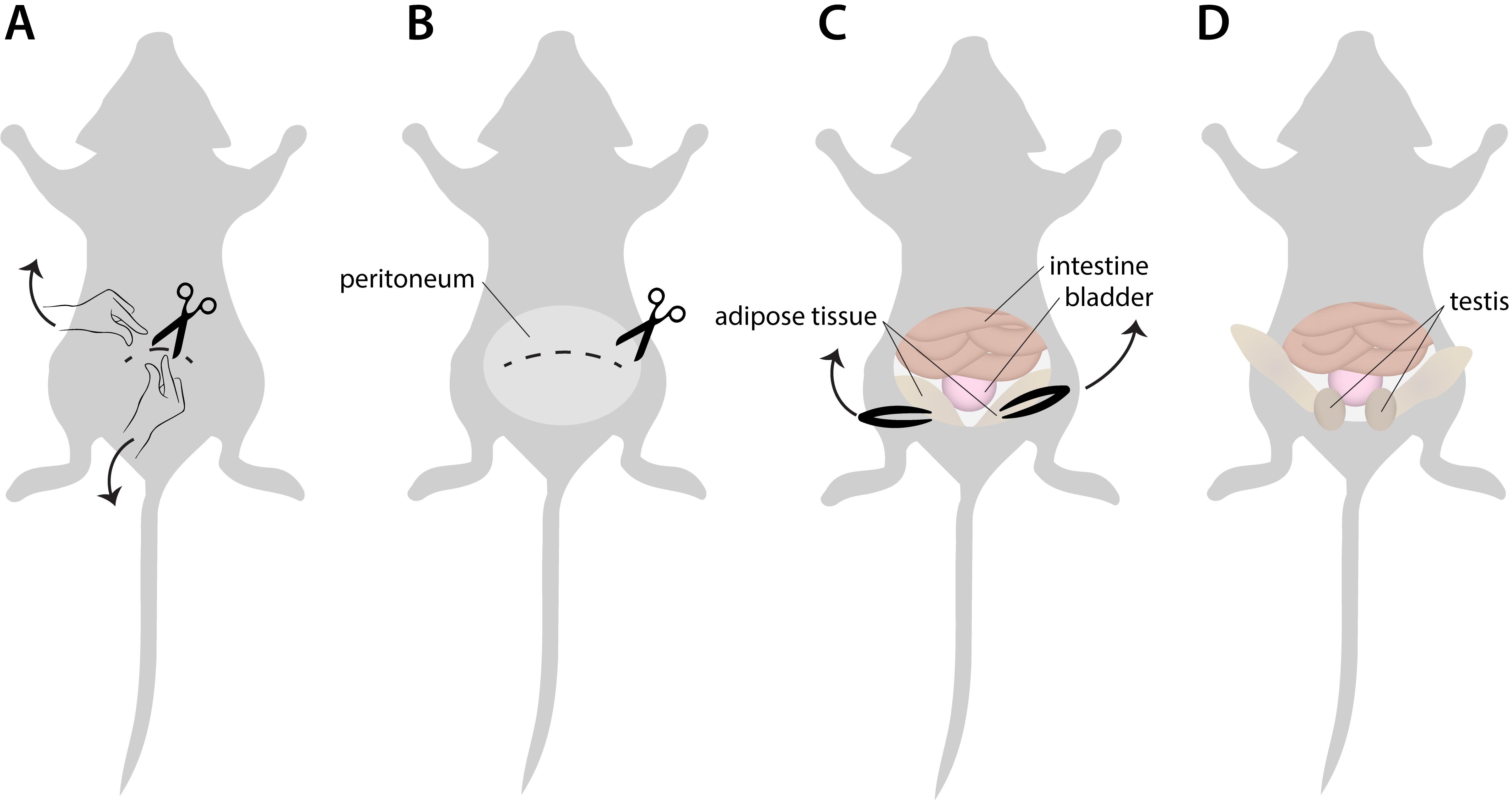
Figure 1. Testis collection. A. Place the sacrificed mouse on its back, wet the skin of the abdomen with 70% ethanol, and open the skin of the lower part of the abdomen with a small cut using scissors. Pinch the skin between the fingers of each hand just above and below the small cut and pull up and downward (along the anterior-posterior axes) to tear the skin further and visualize the peritoneum. This helps to avoid hair contamination. B. Use a tweezer to grasp the peritoneum and use a scissor to cut it open and to enlarge the opening laterally. C. The organs in the lower part of the abdominal cavity are visible at this point (intestine and bladder). The testis is descended and located in the scrotum. Most often, they are not yet visible. To retrieve them from the scrotum, use tweezers to grasp adipose tissue on either side of the bladder and softly pull each of them upwards. D. This will expose the testis, visible as an egg-shaped tissue that should be separated from the surrounding tissue such as the epididymis, blood vessels, etc., using tweezers and scissors to carefully isolate it.Remove the tunica albuginea using tweezers and a fine scissor. This is a fibrous tissue covering the testis. Its removal generates an amorphous mass of testis tubules, connected by interstitial tissue.
Repeatedly place small parts of this tissue mass between two curved tweezers with fine points and rub these against each other in a drop of PBS+ to obtain a cell suspension (for ~5 min) (Video 1, Figure 2A and 2B).
 Video 1. Generation of a cell suspension using curved tweezers with fine points
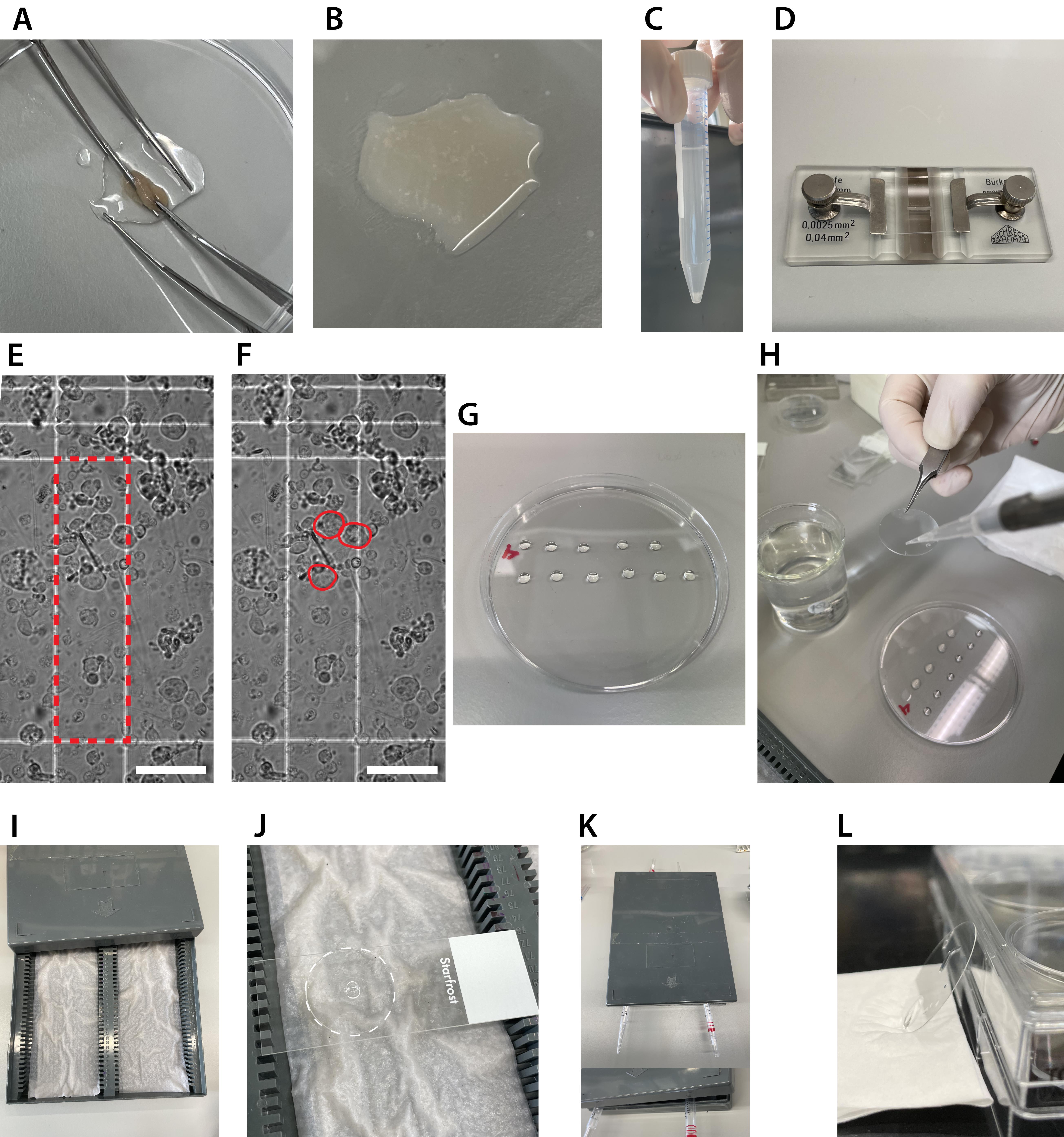
Figure 2. Spreading spermatocyte nuclei for direct stochastic optical reconstruction microscopy (dSTORM). A. Rubbing tissue fragments between two curved tweezers with fine points. B. Cell suspension after ~5 min of repeated rubbing of tissue fragments between the tweezers. C. Example of the result after the remaining tissue fragments have settled down. Only transfer the supernatant. D. Counting chamber. E and F. Example of testicular cells in the counting chamber. Only the large, round cells indicated in F are counted within the red rectangle or crossing the upper and/or right line (E). Scale bar represents 0.05 mm. G. Drops of sucrose in the top lid of a 10 cm dish. H. Adding the sucrose/cell suspension to the PFA drop. I. Humid chamber. J. Coverslip (the edge is accentuated with a white dotted line) with PFA and cells that is positioned on a microscope slide in the humid chamber. For the first hour of incubation, the lid of the humid chamber will be closed. K. Use pipettes to open the humid chamber for the last hour of fixation and drying. L. After the photo Flo wash step, dry the coverslip completely by placing it against the side of a 6-well plate.Bring the whole cell suspension in a 15 mL tube using a pipette and wash the Petri dish with PBS+ several times to collect all cells. Add PBS+ up to a total volume of 10 mL.
Invert the tube twice and wait a few minutes for the larger tissue fragments to settle to the bottom (Figure 2C).
Transfer the supernatant to a clean 15 mL tube using a 10 mL pipette.
Centrifuge for 5 min at 617× g (1,000 rpm).
Remove the supernatant.
Add 1 mL of PBS+ and gently pipette up and down to carefully resuspend the pellet.
Load 10 μL of the cell suspension in the counting chamber (Figure 2D).
Using a phase contrast microscope, count the number of spermatocytes (large, round cells) that are visible at 40× magnification in vertical large rectangles (including cells that cross the upper and/or right side) and calculate the average of 10 rectangle counts. This average is multiplied by 106 to obtain the concentration of cells/mL (Figure 2E and 2F).
Note: When the number of spermatocytes per rectangle is low (e.g., many rectangles with a score of zero), count 20 rectangles to arrive at a more trustworthy average.
Add 1 mL of Hypobuffer (always an equal volume of Hypobuffer and cell suspension) to the cell suspension and wait for 8 min.
Add PBS+ to a total volume of 10 mL and centrifuge for 5 min at 617× g (1,000 rpm).
Remove the supernatant and resuspend the pellet in PBS+ in a volume that yields a concentration of 15 × 106 cells/mL. For example: the average cell count at step A15 was 2; this corresponds to a concentration of 2 × 10⁶ cells/mL. To obtain a concentration of 15 × 106 cells/mL, divide 2 × 106 by 15 × 106 to obtain the resuspension volume (in mL) of PBS+. In this example, you add 133 μL of PBS+ to the pellet.
Make separate drops of 20 μL of 100 mM sucrose in a 10 cm Petri dish and add 10 μL of the cell suspension to each drop (pipette up and down to create a homogenous solution) (Figure 2G).
Hold the coated coverslip (Recipe 7) with a tweezer and scoop it through the PFA to end with a drop of PFA on the coverslip (Video 2).
Video 2.Scooping the coverslip into the PFAPipette the 30 μL cell suspension with sucrose in the PFA drop and disperse the solution by slowly moving the coverslip circularly (Figure 2H, Video 3).
Note: This is easiest if two people work together, one handling the coverslip and the other adding the cell suspension.
Video 3. Dispersing the solution by circular movements of the coverslipPlace the coverslip with the cells upwards on a microscope glass slide in a humid box (Figure 2I and 2J).
Leave the coverslips for 1 h in the humid box with the lid closed.
Generate a small opening by placing the lid on two pipettes and allow the coverslips to slowly dry for 1 h (Figure 2K).
Notes:
When making spreads on microscope glass slides, this second drying step only takes 30 min.
This is a critical step; it is necessary to always check your coverslip under the microscope to assess if cells have attached to the coverslip before continuing. If they are mostly still floating, incubate for 15 or 30 min longer until the majority of cells appear to have attached.
Always remember which side of the coverslip contains the cells, since this is not visible. Once you grab the coverslip with the tweezers, you have to keep track of which side should remain up. Grab the coverslip with a tweezer and wash in 200 mL of 0.08% photo Flo (Recipe 8) by slowly moving it through the solution for 10 s.
Let the coverslips air dry by placing them against the side of a 6-well plate (Figure 2L).
When dry, the coverslips are ready for immunocytochemistry (pause point). For long time storage, place the coverslips in a small Petri dish (with cells upwards) closed with small pieces of tape and store at -80 °C, or continue directly with the immunocytochemistry procedure.
Note: When making spreads on rectangular microscope glass slides, dried slides can be packaged back-to-back in aluminum foil and also stored at -80 °C.
Immunocytochemistry on nuclear spread preparations
Thaw the coverslip for 10 min at RT.
Place the coverslip into a 6-well plate with dH2O between the wells in a box with wet paper (humid chamber for immunocytochemistry). Keep the 6-well plate as much as possible in the box with wet paper during all the next steps.
Wash the coverslip in 2 mL of 1× PBS (Recipe 10) on a shaking plate for 10 min and repeat this two times.
Note: When using spreads on microscope glass slides, use a Coplin jar for washing.
Block the chromatin on the coverslip by adding 700 μL of blocking buffer 1 drop by drop on the coverslip (Recipe 11) and incubate for 20 min.
To perform the three-color staining of SYCP3, RAD51, and DMC1, add 0.5 μL of SYCP3 antibody, 1 μL of DMC1 antibody (from a 1:10 dilution, which is 1 μL of antibody and 9 μL of 1× PBS), and 1 μL of RAD51 antibody (from a 1:10 dilution, which is 1 μL of antibody and 9 μL of 1× PBS) to 100 μL of primary antibody buffer (Recipe 12).
Remove blocking buffer 1 using a pipette. Subsequently, add the primary antibody buffer including antibodies as prepared in step B5.
Cover the coverslip with a small circle of Parafilm that has approximately the same size as the coverslip and place the Parafilm circle on the coverslip with buffer using tweezers for equal distribution.
Incubate the coverslip with the primary antibody overnight at RT.
Note: It is possible to perform incubation also at 4 °C for two nights but, before storing at 4 °C, the coverslip should be incubated for at least 1 h at RT. Before continuing with the protocol on the next day, it should also be incubated at RT for at least 1 h.
Gently remove the Parafilm using tweezers.
Wash the coverslip in 2 mL of 1× PBS on a shaking plate for 10 min and repeat this two times.
Block the coverslip by adding 700 μL of blocking buffer 2 (Recipe 13) and incubate for 20 min.
To perform the three-color staining of SYCP3 (Alexa 647), RAD51 (CF568), and DMC1 (Atto488), add 2 μL of goat anti-guinea pig Alexa 647 antibody (from a 1:10 dilution, which is 1 μL of antibody and 9 μL of 1× PBS), 2 μL of goat anti-rabbit CF568 antibody (from a 1:10 dilution, which is 1 μL of antibody and 9 μL of 1× PBS), and 0.4 μL of goat anti-mouse Atto488 to 100 μL of blocking buffer 2 (Recipe 13). Protect this mix from light before use.
Gently remove the blocking buffer 2 and add the 100 μL of blocking buffer solution including antibodies that was prepared in step B12.
Cover the coverslip with Parafilm (see step B7).
Incubate the coverslip with the secondary antibody solution for 2 h at RT.
Gently remove the Parafilm.
Wash the coverslip in 2 mL of 1× PBS for 10 min on a shaking plate, repeat this twice, and protect it from light by wrapping it in aluminum foil.
Store the coverslip in 2 mL of 1× PBS in a 6-well plate (add water between the wells) in a dark box with wet paper (or a white box covered in aluminum foil) and store at 4 °C until further use.
Notes:
It is recommended to use a fresh immunostained sample for dSTORM. The sample, when stored in a dark box (or a 6-well plate kept in the dark), can last for months, but sample quality can decrease over time.
Two milliliters of PBS is enough for short-time usage but could evaporate when stored longer; please keep in mind to increase this volume when storing the coverslip for longer.
Addition of fiducials to the sample
Sonicate the vial containing the fiducials (TetraSpecksTM) for 20 s.
Pipette 0.5 mL of 1× PBS in an Eppendorf tube.
Place the coverslip in the AttofluorTM cell chamber and close the chamber carefully by screwing.
Note: Be careful with closing the chamber because closing it too loose will cause leakage and closing it too tight will cause the coverslip to break.
Pipette the fiducials at least 10 times up and down.
Add 0.35 μL of the fiducials to the PBS in the Eppendorf tube and mix thoroughly.
Add the fiducials with PBS to the sample in the AttofluorTM cell chamber and make sure that the liquid is dispersed equally. If not, softly tap to the side of the chamber.
Note: The distribution pattern of fiducials among different fields of view is often very variable, despite the thorough mixing of the solution beforehand. Selection of cells with a suitable number of fiducials before starting the actual dSTORM imaging is therefore essential (see step E2).
Add 0.5 mL of 1× PBS to the chamber.
Place the chamber in a 10 cm Petri dish and protect it from light.
Store it at 4 °C overnight to allow fiducials to settle.
Remove the solution with fiducials the next day and replace it with 1 mL of 1× PBS.
Note: The fiducials need to settle down; if this procedure is shortened, not enough fiducials will be visible on the sample, which makes the alignment of the different channels after imaging impossible.
dSTORM microscope setup
Turn on the microscope 1 h before imaging.
Start ZEN Software and turn on all lasers.
Prepare dSTORM buffer: mix 200 μL of 5× glucose (Recipe 16), 10 μL of dSTORM enzymes (Recipe 17), 25 μL of MEA (Recipe 18), and 765 μL of dH2O.
Note: Enzyme and MEA can expire over time, which decreases the blinking capacity during imaging.
Remove PBS from the sample in the AttofluorTM cell chamber and add 1 mL of dSTORM buffer.
Close the chamber with a coverslip.
Notes:
To make sure that the chamber is closed off from air, gently tap against the AttofluorTM cell chamber so that air bubbles that are present rise and become visible just below the top coverslip. Having a small air bubble in the chamber is not harmful and shows that the chamber is properly sealed due to capillary action.
The dSTORM buffer works for a maximum of 4–5 h after preparation. Thereafter, the blinking capacity will decrease and a new dSTORM buffer needs to be prepared and added to the sample.
Add a drop of oil to the 100× 1.46 NA objective.
Place the chamber in the microscope 30 min before imaging to let the dSTORM buffer establish its equilibrium at a stabilized temperature.
dSTORM imaging
Focus on the sample by eye through the oculars using the mercury lamp and appropriate filters.
Search for a nucleus. A good nucleus or cell is characterized by a strong signal of all fluorophores, little to no background signal of fluorophores, and an optimal number of fiducials (at least 5–10, maximum 50). Too few fiducials make the alignment difficult/impossible and too many fiducials interfere with your signal to be imaged.
Check the infrared signal using the camera (continuous mode) since it is not visible through the ocular lens.
Set up the microscope for three channels; in our case, by selecting the laser 488, 561, or 642 (“on” in Figure 3) and the corresponding filter block BP 495-575, BP 570-650, or LP655 (the latter is visibly selected in Figure 3).
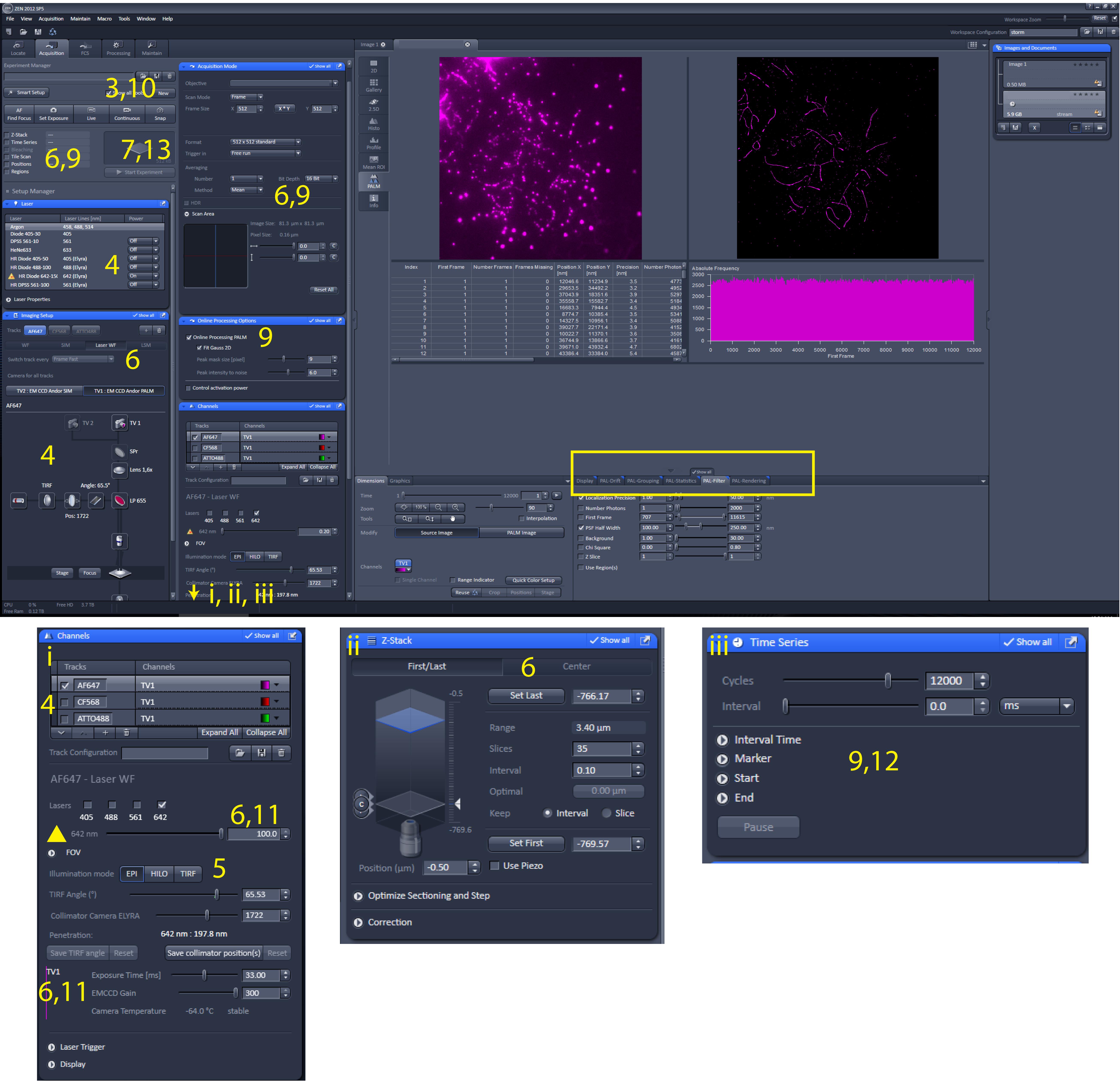
Figure 3. Screenshot of ZEN software. Screenshot of ZEN software during direct stochastic optical reconstruction microscopy (dSTORM) imaging and pre-processing to reconstruct dSTORM image. The yellow numbers indicate the relevant location on the screen corresponding to the steps described in Section E. The yellow rectangle indicates the relevant location on the screen related to Data analysis “Pre-processing to reconstruct dSTORM image.” i, ii, and iii indicate screen parts that become (completely) visible when sliding down the bar that is on the right side of the acquisition parameters column.Only for the first nucleus: set the TIRF angle by focusing on the sample using the AF647 channel and select EPI as illumination mode. Move the TIRF angle slider to the right until the signal disappears; this setting is just beyond the optimal TIRF angle. Then, move the slider to the left and stop when the penetration depth indicated in the software is between 190 and 200 nm. At this TIRF angle, only a small region just above the coverslip is illuminated, giving high signals and no background from out-of-focus contributions. Repeat this for CF568 and ATTO488.
Note: A penetration depth between 190 and 200 nm should illuminate the full sample but not more. This can be achieved by moving from no signal until the brightest signal of the stained protein is visible.
Take a snapshot (z-stack) of the nucleus: select all channels one by one (Figure 3, screen i) and set the following settings: laser power = 2% (indicated with the yellow triangle), exposure time = 100 ms, EMCCD gain = 100 a.u., light path (Figure 3, main screenshot, under Imaging setup bar): switch track every = z-stack, Under acquisition mode bar: averaging = 2. Select the option Z-stack (Figure 3, main screenshot, top left, and Figure 3, screen ii), ensure that the image is in focus, and use the z-stack Center option. Thereafter, press center to put the z-stack in the middle of the cell. Select settings to make a z-stack with 35 slices of 0.110 μm.
Notes:
When the signal is saturated, lower the gain.
These settings depend on the specific microscope and camera used. This is a low laser power setting to avoid monitor bleaching.
Press Start Experiment .
Save the snapshot as a .czi file using file save (Exp1_snap.czi). The use of an experiment name is essential for the data analysis. In this example, we choose to use Exp1 as our experiment name.
Continue with the dSTORM imaging by selecting the following: Online Processing PALM (peak mask size = 9 pixels, peak intensity noise = 6) (Figure 3, main screenshot, under Online processing Options ), and under acquisition mode bar: averaging = 1, deselect “Z-Stack” (Figure 3, main screenshot, top left) and instead select Time series (12,000 frames).
Focus on the observed image with the AF647 track selected.
Adjust settings as follows (Figure 3, screen i): laser power = 100%, exposure time = 33 ms, EMCCD gain = 300 a.u., and press Continuous (Figure 3, main screenshot, top left). This will directly increase the signal intensity followed by an overall decrease of the signal, and finally in clearly blinking fluorophores on the screen. Press Stop when all fluorophores blink well, which can depend on the dSTORM buffer quality or the type of fluorophore. Under normal conditions, this takes a few minutes for Alexa 647.
Note: These settings may have to be adapted depending on the microscope and camera. This setting pushes all fluorophores into a dark state, but high laser power can also bleach fluorophores. If too many fluorophores are bleached, lowering the laser power is essential. The camera is most sensitive when the gain is set at maximum (for EMCCD cameras) and when an exposure time is chosen that allows recording of individual separated blinking events. A longer exposure time will record more photons and thus lead to increased localization precision, but also yields a higher chance of recording multiple overlapping blinking events, which should be prevented.
Set the experiment to time series (Figure 3, screen iii) and define a series of 12,000 frames with 0 ms interval.
Press Start Experiment .
During the ongoing recording of 12,000 frames, make sure that the number of detections per frame (First Frame) stays approximately constant. When detection frequency decreases, this may be due to loss of focus or bleaching of fluorophores. Loss of focus can be assessed in the wide field image, and focus should be adjusted when necessary. If focus is corrected and detection frequency still decreases, bleaching of fluorophores can be slowed down by lowering the laser power to 90%, or an even lower percentage, but not lower than 70%.
Notes:
For Alexa 647, most often it is not necessary to adjust the laser power.
Systems with hardware autofocus are highly recommended.
Save the movie as a .czi file (Exp1_Ch1.czi).
Repeat steps E8–E15 for the CF568 (Exp1_Ch2.czi).
Note: Proper dSTORM imaging of the CF568 fluorophore normally requires a bit longer waiting time before it starts to blink properly, compared with Alexa 647 (5–8 min). Make sure not to start recording too early, to ensure the optimal yield of blinking events.
Repeat steps E8–E15 for ATTO488 (Exp1_Ch3.czi).
Notes:
Atto488 bleaches very fast. Therefore, when the high laser power is switched on at step E11, wait a few seconds and then directly start the experiment (steps E12–E13). During imaging, you will rapidly see a drop in the number of localization events per frame, and therefore the laser power should be lowered in steps of 10% to a minimum of 70% already during the first 1,000–1,500 frames. Green fluorophores are less suitable than longer wavelength fluorophores for dSTORM imaging, and therefore green dyes will give lower resolution images. This should be taken into account when choosing target proteins and their corresponding fluorescent label.
Another option to stimulate the blinking of the green dye is to use the 405 nm laser at very low power to release molecules from their dark state and increase the number of localization events.
Data analysis
Pre-processing steps to reconstruct the dSTORM image
Notes:
Install the Plugin STORM_Tools.jar in Fiji and RTools and SMoLR in R. Also, open the custom data analysis pipelines in Fiji and R.
Test data for the data analysis pipeline is available via BioImage Archive (http://www.ebi.ac.uk/bioimage-archive) under accession number S-BIAD627.
The use of an experiment name (e.g., the name of the experiment like Exp1 in the test data) is essential for the scripts to work properly.
Additional information about the SMoLR package can be found at https://github.com/ErasmusOIC/SMoLR and https://htmlpreview.github.io/?https://github.com/ErasmusOIC/SMoLR_data/blob/master/SMoLR.html . Additional help on each SMoLR function can be accessed by entering a “?” followed by the name of the specific function (i.e., ?SMOLR_PLOT).
Re-open the movies in the ZEN Software.
Perform a drift correction as follows. PAL drift: select model-based approach and press apply two times (Figure 3 yellow square). Save the table as a .txt file by right-clicking on the table. Repeat this for every channel (Exp1_Ch1.txt, Exp1_Ch2.txt, Exp1_Ch3.txt).
Note: The drift correction is needed to correct for small drifts that occurred during imaging.
Perform grouping as follows. PAL Group: max on time = 50, off gap = 2, capture radius = 4 pixels (Figure 3 yellow square). Save the table as a .txt file by right-clicking on the table. Repeat this for every channel (Exp1_ Ch1_g.txt, Exp1_Ch2_g.txt, Exp1_Ch3_g.txt).
Note: Grouping is essential to couple blinking events from the same fluorophore within a specific time range.
The pre-processing continues in Fiji, where you start with seven files: a z-stack image (Exp1_snap.czi) and, per channel, a drift-corrected localization file (Exp1_Ch1.txt, Exp1_Ch2.txt, Exp1_Ch3.txt) and a drift-corrected and grouped localization file (Exp1_Ch1_g.txt, Exp1_Ch2_g.txt, Exp1_Ch3_g.txt). Align the different channels in Fiji using the script Align_dSTORM_channels by using a gap of 50 and a track length of 70 (Figure 4A). The ungrouped localization files (Exp1_Ch1.txt, Exp1_Ch2.txt, Exp1_Ch3.txt) are used to identify fiducials, and the grouped location files (Exp1_Ch1_g.txt, Exp1_Ch2_g.txt, Exp1_Ch3_g.txt) are used for further data analysis. This generates two transformation files (Exp1_Ch2_transformation.txt and Exp1_Ch3_transformation.txt) containing the transformation matrix to align Ch2 and Ch3 with Ch1 as a template and two localization files containing the transformed localizations from Ch2 and Ch3 (Exp1_Ch2_gt.txt and Exp1_Ch3_gt.txt).
Notes:
Name the channels based on wavelength, whereby channel 1 corresponds to the highest wavelength. In case you only have two channels, exclude channel 3.
When the number of fiducials found is lower than 3 (or the alignment turned out not to be correct), increase the gap size or decrease the track length.
The script Align_dSTORM_channels is based on the DoM Plugin (Katrukha et al., 2022).
The directory asked for in the script is the location where the .txt files are stored.
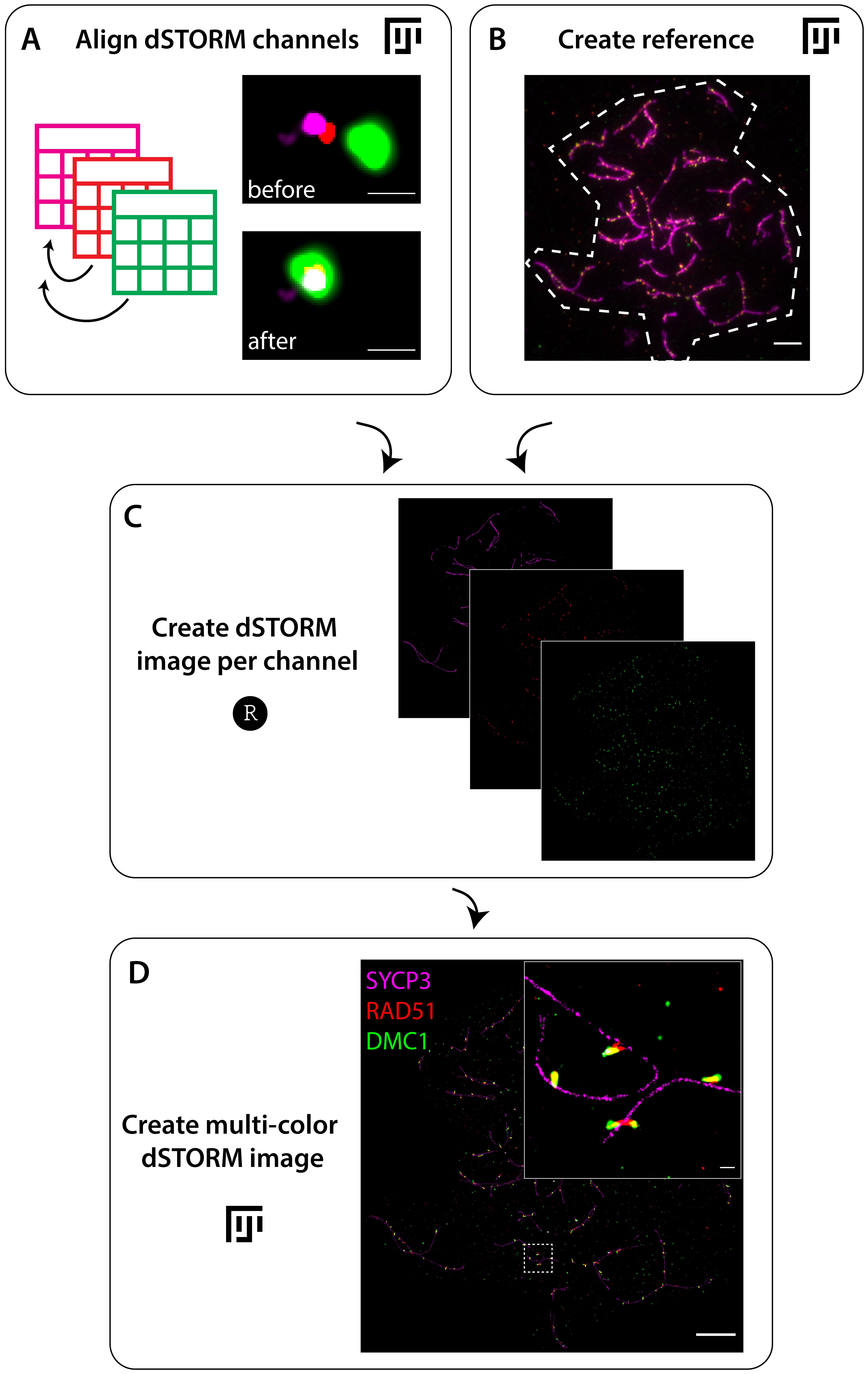
Figure 4. Flowchart of pre-processing to reconstruct direct stochastic optical reconstruction microscopy (dSTORM) image. A. Start with the alignment of dSTORM channels by aligning the localization tables in Fiji using the script Align_dSTORM_channels . An example of a fiducial before and after alignment is shown (steps A1–A4). B. Next, determine the outline of the nucleus in the z-stack image to generate a reference in Fiji using the script Create_reference (step A5). C. The aligned localization tables and the reference are used in R using the R script Create dSTORM image per channel to generate the dSTORM images per channel (step A6). D. Finally, the separate dSTORM images per channel are combined in Fiji to create a multi-color dSTORM image using the script Create_multi-color_dSTORM_image (step A7). An example of a three-color dSTORM image of a spread spermatocyte nucleus immunostained for SYCP3 (magenta), RAD51 (red), and DMC1 (green) is shown, including an enlargement of the region indicated with the dotted square. Scale bar represents 100 nm (A), 250 nm (D enlargement), and 5 μm (B, D).Create a reference for the dSTORM image by using the z-stack image in Fiji and running the script Create_reference (Figure 4B). In short, select the z-position with the best focus for each channel, merge these single images, and save this image (Exp1_Composite.tif). Determine the border of the nucleus saved as a region of interest (ROI) (Exp1_Roi.roi) including its characteristics (Exp1_Roi_characteristics.csv). This reference is created to reduce computational time in the following steps of the pre-processing.
Notes:
To open the .czi file via Bio-Formats (Plugins/Bio-Formats/Bio-Formats Importer), set the following settings in Import Options (View stack with: Hyperstack, Color mode: Colorized, and select “Autoscale”).
The z-position can be found in the left upper corner of the image (z:1/35).
Use R and the package SMoLR to process the transformed localization files into a dSTORM image per channel by running the script Create dSTORM image per channel of the R script (Figure 2C). In short, the localization files are imported and converted to a data frame. The localizations within the previously selected nucleus ROI are transformed into an image (Exp1_Ch1.tif, Exp1_Ch2.tif, Exp1_Ch3.tif).
Notes:
Manually set the directory in the R script.
Generation of the images in R is a time-consuming step.
Combine the individual images of each channel in Fiji using the script Create_multi-color_dSTORM_image (Figure 4D). In short, this script uses Bio-Formats to import individual images. For each image, the image intensity is converted into a 16-bit image. Also, each image is colored (Ch1 = magenta, Ch2 = red, Ch3 = green) and all individual images are combined into one image, which is saved (Exp1_Ch1_Ch2_Ch3.tif).
Note: The script adjusts the brightness/contrast of the image using the auto settings. In case this is not correct, decrease the maximum value and/or increase the minimum value using the B&C control (Image > Adjust > Brightness/Contrast).
Check if the channels are correctly aligned, as shown in the example in Figure 4A.
Recombination foci analysis
Identify regions of interest (ROIs) that display RAD51 and/or DMC1 signals in Fiji using the script ROI_selection (Figure 5A). The details of this script were previously described in the Material and Methods section under the heading Recombination foci analysis of Koornneef et al. (2022). In short, this script uses the three-color dSTORM image (Exp1_Ch1_Ch2_Ch3.tif) and performs a semi-automatic identification of ROIs containing both RAD51 and/or DMC1 nanofoci using specific thresholds for focus size and SYCP3 signal. The default thresholds for focus size are 500 pixels for RAD51 and 300 pixels for DMC1, and the radius of each ROI is set at 375 nm. This whole procedure generates a set of all identified ROIs (Exp1_allRois.zip), a set of ROIs after manual adaption (Exp1_RoiSet.zip), a transformed set of ROIs after manual adaptation (Exp1_RoiSet_t.zip), and a file containing specific characteristics of each ROI (Exp1_RoiSet_t_characteristics.csv).
Note: To manually add ROIs (after visual inspection of all identified ROIs in the image), use the script Manual ROI selection with a radius of 375 nm. To select a ROI, click on the center of the region. Press T to add this ROI to the ROI Manager. To remove an ROI from the ROI Manager, select the ROI and press Delete. To stop the macro Manual ROI selection, finish the ROI_selection macro or press shift and click at a random position in the image.
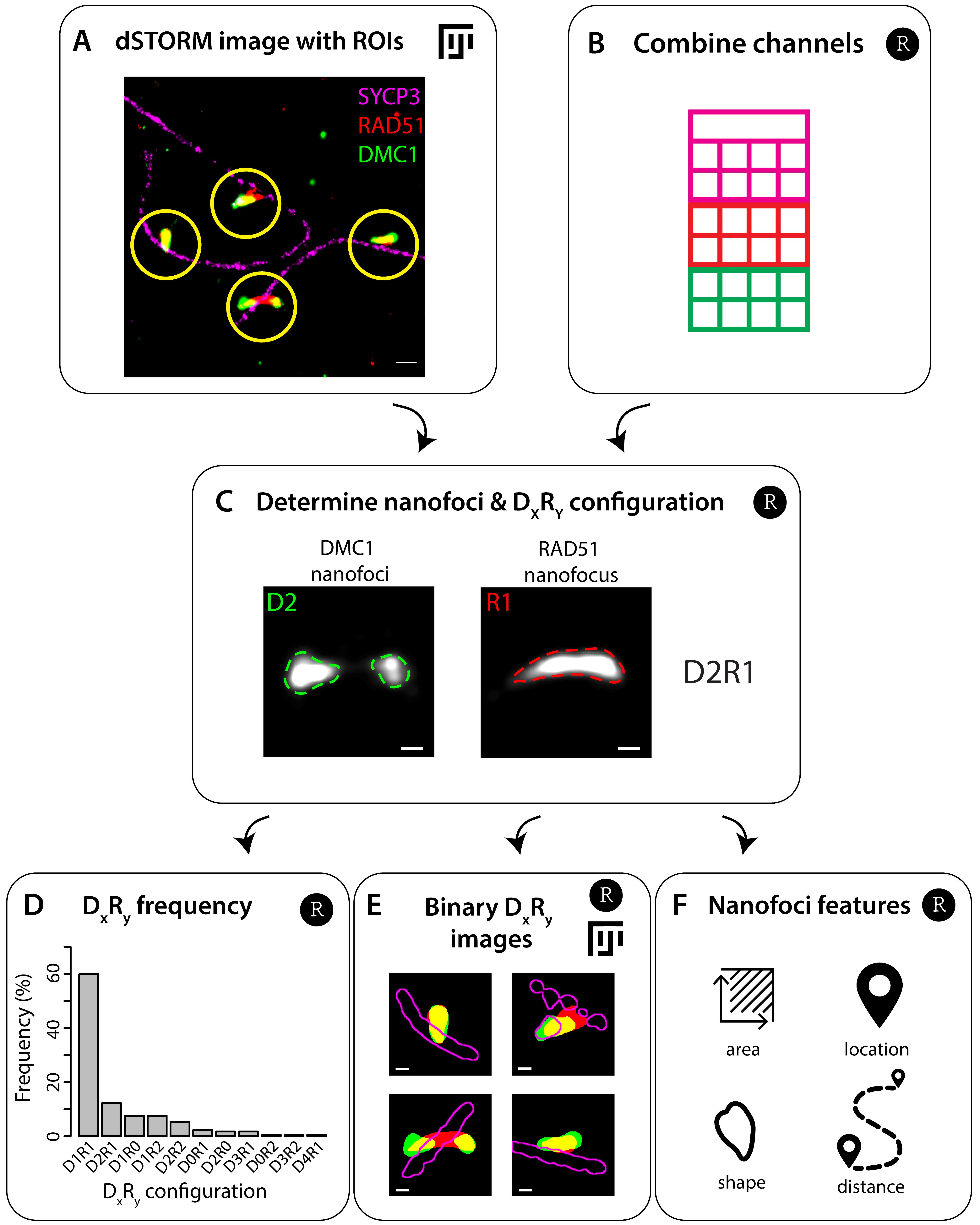
Figure 5. Flowchart of recombination foci analysis. A. Select regions of interest (ROIs) containing RAD51 and DMC1 foci in the three-color direct stochastic optical reconstruction microscopy (dSTORM) image in Fiji using the script ROI_selection (step B1). An example of part of a three-color dSTORM image of a spread spermatocyte nucleus immunostained for SYCP3 (magenta), RAD51 (red), and DMC1 (green). ROIs of 750 nm diameter are indicated as yellow circles. B. Combine aligned localization files of different channels into one data frame in R using the script Combine channels (step B2). C. The combined localization file and the ROIs are combined to generate small dSTORM localization files of every ROI, whereafter the clusters of localizations (termed nanofoci) are determined. The number of nanofoci within an ROI determines the DxRy configuration correlating with x DMC1 nanofoci and y RAD51 nanofoci. The example is a kernel density estimation of a ROI, whereby the dashed green and red lines visualize the binary outline of the nanofoci. This ROI has a D2R1 configuration, as it contains two DMC1 nanofoci and a single RAD51 nanofocus. All these steps are performed in R using the script Analysis of ROIs (step B3). D, F. The DxR y configuration can be used to determine the frequency (D, step B3) or create binary images of every ROI (E, step B4). Also, features of RAD51 and DMC1 nanofoci can be measured (F, step B5). Scale bar represents 250 (A) and 100 nm (C, E).Combine the localization files from each channel into one data frame in R (Exp1_alldata.txt), using the script Combine Channels (Figure 5B).
Process the ROIs in R into DxRy configurations using the script Analysis of ROIs (Figure 5C). In short, a list is generated in which for each ROI all the localization events corresponding to all channels are documented (Exp1_data_sub.RData). Next, a kernel density estimation is performed on the subset of localization data from each ROI to cluster localization events (Exp1_kde.RData). A signal density threshold [0.05 (axes component) or 0.15 (recombinases) localizations/nm2] is used to create binary clusters termed nanofoci. The number of nanofoci within a ROI determines the DxRy configuration and thereby also the DxRy frequency that can be then determined for each nucleus (Figure 5D). Nanofoci smaller than 1,250 nm2 are excluded. Also, a statistics file (Exp1_sf.RData) is generated with details about the ROIs and their DxRy configuration information.
Notes:
Manually set the directory, the threshold for the kernel density estimate, and the threshold for the area in the R script.
Generation of data_sub.RData and kde.RData is a time-consuming step.
Optional: Generate binary images of individual ROIs in R using the script Generate binary DxRy images .
Note: The colors (red, green, and blue) in the generated images represent channels 1, 2, and 3, respectively.
Features of nanofoci (like the position and the number of localizations) can be found in the cluster parameters of kde.RData (e.g., for ROI number 1, use kde[[1]]$clust_parameters). Features of nanofoci (like area and shape) can be found in features (e.g., for channel 3 in ROI number 1, use features[[1]]$channel_3 and “x.0.s.area” or “x.0.m.eccentricity”). Also, other features (like distances to other nanofoci) can be calculated using the data_sub.RData and kde.RData, but require additional processing.
Note: Manually set the directory and threshold for the area in the R script.
Acknowledgments
This protocol was used to obtain the data published in PLOS Genetics (Koornneef et al., 2022).
We would like to thank E. Sleddens-Linkels for help with image acquisition and videos to document the meiotic nuclei spreading procedure. We would like to thank I. de Bruin for testing the protocol including the analysis pipeline as a new user and R. Benavente for providing the SYCP3 antibody.
Competing interests
All authors declare they have no conflicts of interest or competing interests.
Ethical considerations
All procedures were in accordance with the European guidelines for the care and use of laboratory animals (Council Directive 86/6009/EEC). All animal experiments were approved by the local animal experiments committee DEC (Dutch abbreviation: Dier Experimenten Commissie) Consult and animals were maintained under the supervision of the Animal Welfare Officer.
References
- Alsheimer, M. and Benavente, R. (1996). Change of Karyoskeleton during Mammalian Spermatogenesis: Expression Pattern of Nuclear Lamin C2 and Its Regulation. Exp. Cell. Res. 228(2): 181–188.
- Barlow, A. L., Jenkins, G. and ap Gwynn, I. (1993). Scanning electron microscopy of synaptonemal complexes. Chromosome Res. 1(1): 9–13.
- Betzig, E., Patterson, G. H., Sougrat, R., Lindwasser, O. W., Olenych, S., Bonifacino, J. S., Davidson, M. W., Lippincott-Schwartz, J. and Hess, H. F. (2006). Imaging Intracellular Fluorescent Proteins at Nanometer Resolution. Science 313(5793): 1642–1645.
- Cremer, C. and Cremer, T. (1978). Considerations on a laser-scanning-microscope with high resolution and depth of field. Microsc. Acta. 81(1): 31–44.
- Essers, J., Hendriks, R. W., Wesoly, J., Beerens, C. E., Smit, B., Hoeijmakers, J. H., Wyman, C., Dronkert, M. L. and Kanaar, R. (2002). Analysis of mouse Rad54 expression and its implications for homologous recombination. DNA Repair 1(10): 779–793.
- Katrukha, E., Teeuw, J., bmccloin and den Braber, J. (2022). ekatrukha/DoM_Utrecht: Detection of Molecules 1.2.5 (1.2.5). Zenodo.
- Koornneef, L., Slotman, J. A., Sleddens-Linkels, E., van Cappellen, W. A., Barchi, M., Tóth, A., Gribnau, J., Houtsmuller, A. B. and Baarends, W. M. (2022). Multi-color dSTORM microscopy in Hormad1-/- spermatocytes reveals alterations in meiotic recombination intermediates and synaptonemal complex structure. PLos Genet. 18(7): e1010046.
- Paul, M. W., de Gruiter, H. M., Lin, Z., Baarends, W. M., van Cappellen, W. A., Houtsmuller, A. B. and Slotman, J. A. (2019). SMoLR: visualization and analysis of single-molecule localization microscopy data in R. BMC Bioinf. 20(1): e1186/s12859-018-2578-3.
- Peters, A. H., Plug, A. W., van Vugt, M. J. and de Boer, P. (1997). A drying-down technique for the spreading of mammalian meiocytes from the male and female germline. Chromosome Res 5(1): 66–68.
- R Core Team. (2018). R: A language and environment for statistical computing.
- Rust, M. J., Bates, M. and Zhuang, X. (2006). Sub-diffraction-limit imaging by stochastic optical reconstruction microscopy (STORM). Nat. Methods 3(10): 793–796.
- Schindelin, J., Arganda-Carreras, I., Frise, E., Kaynig, V., Longair, M., Pietzsch, T., Preibisch, S., Rueden, C., Saalfeld, S., Schmid, B., et al. (2012). Fiji: an open-source platform for biological-image analysis. Nat. Methods 9(7): 676–682.
- Slotman, J. A., Paul, M. W., Carofiglio, F., de Gruiter, H. M., Vergroesen, T., Koornneef, L., van Cappellen, W. A., Houtsmuller, A. B. and Baarends, W. M. (2020). Super-resolution imaging of RAD51 and DMC1 in DNA repair foci reveals dynamic distribution patterns in meiotic prophase. PLos Genet. 16(6): e1008595.
Article Information
Copyright
© 2023 The Author(s); This is an open access article under the CC BY-NC license (https://creativecommons.org/licenses/by-nc/4.0/).
How to cite
Koornneef, L., Paul, M. W., Houtsmuller, A. B., Baarends, W. M. and Slotman, J. A. (2023). Three-color dSTORM Imaging and Analysis of Recombination Foci in Mouse Spread Meiotic Nuclei. Bio-protocol 13(14): e4780. DOI: 10.21769/BioProtoc.4780.
Category
Developmental Biology > Reproduction > Germ cell
Do you have any questions about this protocol?
Post your question to gather feedback from the community. We will also invite the authors of this article to respond.