- Protocols

- Articles and Issues
- For Authors
- About
- Become a Reviewer

Relative Membrane Potential Measurements Using DISBAC2(3) Fluorescence in Arabidopsis thaliana Primary Roots
Published: Vol 13, Iss 14, Jul 20, 2023 DOI: 10.21769/BioProtoc.4778 Views: 1728
Reviewed by: Samik BhattacharyaIgnacio Lescano
Original research article
The authors used this protocol in:
Sep 2021
Advertisement


Protocol Collections
Comprehensive collections of detailed, peer-reviewed protocols focusing on specific topics


Abstract
In vivo microscopy of plants with high-frequency imaging allows observation and characterization of the dynamic responses of plants to stimuli. It provides access to responses that could not be observed by imaging at a given time point. Such methods are particularly suitable for the observation of fast cellular events such as membrane potential changes. Classical measurement of membrane potential by probe impaling gives quantitative and precise measurements. However, it is invasive, requires specialized equipment, and only allows measurement of one cell at a time. To circumvent some of these limitations, we developed a method to relatively quantify membrane potential variations in Arabidopsis thaliana roots using the fluorescence of the voltage reporter DISBAC2(3). In this protocol, we describe how to prepare experiments for agar media and microfluidics, and we detail the image analysis. We take an example of the rapid plasma membrane depolarization induced by the phytohormone auxin to illustrate the method. Relative membrane potential measurements using DISBAC2(3) fluorescence increase the spatio-temporal resolution of the measurements and are non-invasive and suitable for live imaging of growing roots. Studying membrane potential with a more flexible method allows to efficiently combine mature electrophysiology literature and new molecular knowledge to achieve a better understanding of plant behaviors.
Key features
• Non-invasive method to relatively quantify membrane potential in plant roots.
• Method suitable for imaging seedlings root in agar or liquid medium.
• Straightforward quantification.
Keywords: AuxinBackground
Establishment of a membrane potential is essential to support cell function in all living organisms. In plants, membrane potential reflects the electrical difference between the cytoplasm and the apoplast (in root epidermis between -120 and -160 mV, Sze et al., 1999; reviewed in Serre et al., 2021). This phenomenon is mostly driven by the H+-ATPases proton pumps, which extrude positively charged protons from the cytoplasm to the apoplast (Sze, 1985), resulting in negative membrane potentials (Sze et al., 1999). These negative membrane potentials are essential for ion transport across the plasma membranes, and thus play an important role in plant nutrition, growth, and development (Tyerman and Schachtman, 1992; Ragel et al., 2019). Reflecting the spectacular ability of plants to adapt to changing local environments, membrane potential can be quickly shifted from the resting potential value to a hyperpolarized (more negative) or a depolarized (more positive) state. Responses vary according to the stimuli and can potentially lead to stress-induced electrical signaling (Mudrilov et al., 2021). For example, salt stress (NaCl) causes a quick and massive entry of positively charged sodium ions into the root tissues, triggering a leak of potassium ions outside the cells to counterbalance the membrane depolarization (for review, see Cuin et al., 2008). Equally, the hormone auxin triggers almost instantaneous membrane depolarization in roots, leading to root growth inhibition by mechanism(s) still not fully understood (Tretyn et al., 1991; Dindas et al., 2018 and 2020, Paponov et al., 2019; Li et al., 2021; Serre et al., 2021; Qi et al., 2022; Roosjen et al., 2022).
Membrane potential is traditionally measured by impaling electrodes into living tissues (Shabala et al.,2005). While this method gives extremely accurate and quantitative measurements, it is invasive, requires dedicated equipment, and is not fully adapted to the study of growing tissues for a long period of time. Furthermore, the reported potential only concerns one cell and thus limits high resolution spatio-temporal studies.
To circumvent these challenges, we reviewed the literature and available voltage reporter dyes. We selected DISBAC2(3) for its uniform staining of roots and lack of obvious toxicity (Serre et al., 2021). This staining method allowed us to relatively observe membrane potential over time in different tissues. However, the method does not give actual potential values (in mV), lacks sensitivity in strongly hyperpolarized states, and so should always be used in comparison to roots observed under control conditions.
Here, we explain how to analyze relative changes in membrane potential using confocal fluorescence microscopy, taking as an example the imaging of rapid auxin-induced cellular depolarization in Arabidopsis thaliana primary root. We describe how to prepare experiments for imaging of the membrane potential in microfluidics to observe the first instants of the response, as well as imaging in agar media for observation of established responses. Microfluidics is adapted to this type of observation, as each plant can be observed first in control and then in treatment condition, granting internal control fluorescence intensities for every seedling.
The protocols detailed here can be adapted for other dyes to study dynamic events in A. thaliana roots in response to various (a)biotic stimuli.
Materials and reagents
General
Arabidopsis thaliana wildtype Columbia-0 (Col-0) sterile seeds
Porous tape 1.25 cm large (Duchefa, Leucopore, L3302)
Autoclaved wooden toothpicks (any supermarket)
Square Petri dishes (e.g., 15 mm × 15 mm or 10 mm × 10 mm, any brand)
1.5 mL tubes (any brand)
15 mL tubes (any brand)
0.5 mL tubes (any brand)
96% ethanol (Sigma, catalog number: 1.59010), store at room temperature in a flame-protective cabinet
Auxin 3-indoleacetic acid (IAA) (Sigma-Aldrich, catalog number: I2886-5G), store at -20 °C
Murashige and Skoog (MS) medium (Duchefa, catalog number: M0221.0050), store at room temperature
Plant agar (Duchefa, catalog number: P1001), store at room temperature
Sucrose (Duchefa, catalog number: S0809), store at room temperature
MES (Duchefa, catalog number: M1503.0100), store at room temperature
1 M KOH (Sigma-Aldrich, catalog number: 06103), store at room temperature
DISBAC2(3) (Invitrogen, Thermo Fisher, catalog number: B413), store at -20 °C in dark
DMSO (Sigma-Aldrich, catalog number: 94563), store at room temperature
Fluorescein Dextran 10 K MW (Thermo Fisher, Invitrogen, catalog number: D1821)
DISBAC2(3) master stock (see Recipes)
DISBAC2(3) working aliquots (see Recipes)
70% ethanol (approximately) prepared from 96% ethanol (see Recipes)
500 mL of buffered liquid 1/2 MS (see Recipes)
500 mL of buffered solid 1/2 MS (see Recipes)
IAA 10 mM stock (see Recipes)
IAA 100 μM solution (see Recipes)
Fluorescent tracer (to follow treatment arrival in microfluidics) (see Recipes)
Specific to agar media experiments
Round 9 cm diameter Petri dishes (e.g., SterilinTM, Thermo Fisher, catalog number: 101R20)
NuncTM Lab-TekTM II microscopy chambers (VWR, catalog number: 734-2055) or 3D printed (see https://cellgrowth-lab.weebly.com/3d-prints.html)
Specific to microfluidic experiments
Microfluidic chips suited for A. thaliana root imaging (e.g., Grossmann et al., 2011; Fendrych et al., 2018; Serre et al., 2021; for review, see Yanagisawa et al., 2021)
Filtering system (Nalgene, P-Lab, N325045)
0.45 μm pore size 47 mm diameter round filtering membrane (Macherey-Nagel, P-Lab, M680447)
Equipment
Precision scale (any brand)
Vortex bench mixer (any brand)
Sterile laminar flow hood (any brand)
Lab scale (any brand)
Thin tweezers (Dumont No.5, Youlab, F003)
Autoclave (any brand)
pH meter (any brand)
Stirring magnetic rod and magnetic mixer (e.g., 2MAG, Dutscher, catalog number: 699010)
Autoclavable 0.5 L borosilicate glass bottles (e.g., SLS, Dutscher, catalog number: 257065)
500 mL graduated cylinder (any brand, plastic or glass)
1,000 mL beaker (any brand, plastic or glass)
Thin spatula (e.g., Heathrow, Dutscher, catalog number: 037874)
Growth room set in long days [e.g., 23 °C by day (16 h), 18 °C by night (8 h), 60% humidity, and light intensity of 120 μmol photons m-2·s-1]
Confocal microscope setup (see below)
Observation of the membrane potential with DISBAC2(3) staining requires a confocal laser or spinning disk microscope (with a 515 nm source of excitation). Here, we present an example based on our microscopy setup. Spinning disk confocal microscopy is particularly adapted to the imaging of fast responses in high spatio-temporal resolution, as the images are acquired under short exposure times. Moreover, the use of vertical inverted stage microscopy allows to keep the seedlings in their natural orientation (towards gravity) and thus avoid bias based on putting the seedlings on the horizontal plane (von Wangenheim et al., 2017).
Microscope body: Axio Observer 7 inverted (Zeiss); the microscope was set up on its back to obtain a vertical stage (details in von Wangenheim et al., 2017; Zeiss also provides custom mounting on request).
Spinning disk: CSU-W1-T2 spinning disk unit with 50 μm pinholes (Yokogawa)
Excitation source: VS-HOM1000 excitation light homogenizer (Visitron Systems)
Objective: Plan-Apochromat × 20/0.8 (Zeiss)
Detection: PRIME-95B Back-Illuminated sCMOS camera 1,200 × 1,200 pixels (Photometrics)
For microfluidic only: microfluidic pressure driven flow setup
We also describe a protocol to prepare media to observe membrane potential using microfluidics. There are a multitude of microfluidic (or perfusion) setups possible based on manufacturer, budget, and need. The same for the production of microfluidic chips. A detailed protocol describing the establishment of a microfluidic setup and the microfluidic chip production is thus out of scope of this protocol. For an example of microfluidic setup using manually closable and reusable chips, see https://www.elveflow.com/microfluidic-applications/microfluidic-cell-culture/microfluidic-microscopy-imaging/. Note that any microfluidic chip adapted to A. thaliana would work, either conventional glass coverslip–sealed microfluidic chips (e.g., Grossmann et al., 2011; Fendrych et al., 2018; for review, see Yanagisawa et al., 2021) or manually closed microfluidics chips (Serre et al., 2021).
Software
Microscopy imaging software (here, we used Visiview, Visitron, https://www.visitron.de)
ImageJ (v1.53t) Fiji (v2.9.0) (Schindelin et al., 2012)
LibreOffice Calc (https://www.libreoffice.org/) or Microsoft Office Excel (https://www.microsoft.com/fr-fr/microsoft-365/microsoft-office)
R (R Core Team, 2022, https://www.R-project.org/) with the nparcomp (Konietschke et al., 2015) package installed
R studio IDE (optional, https://posit.co/)
Python in the Anaconda distribution platform [tested with Python v3.8, https://www.anaconda.com/products/distribution)] with Spyder IDE (tested with v5.2.2, command: conda install spyder) and installed Seaborn package (tested with v0.11.2, command: conda install seaborn)
Optional: Inkscape
Procedure
Procedure to grow the seedlings for agar experiments and manually closed microfluidic chips
Sterilize A. thaliana Col-0 (or line of interest) seeds with the method of your choice (e.g., chlorine gas; Lindsey et al., 2017).
If the buffered solid 1/2 MS (see Recipes) is solidified, dissolve it completely in the microwave with the lid half unscrewed. If the medium has been kept at 60 °C after sterilization, proceed to the next step.
Critical: The following steps have to be carried out under a sterile laminar flow hood.
Pour 50 mL of buffered solid 1/2 MS into a square Petri dish and allow to solidify (approximately 15 min)
Place approximately 10–20 sterilized Col-0 seeds (or line of interest) in a row (approximately 3 cm from the top) using a sterilized toothpick (or method of your choice).
Close and seal the Petri dish with micropore tape.
Transfer the plate to 4 °C for two days for stratification.
Transfer the plate to the growth room for 4/5 days (primary root length between 2 and 4 cm). Note that seedlings need to fit the microscopy chamber.
Note: Given the short-term aspect of the observations carried out, the experiments are performed in a non-sterile environment.
Experiments with agar medium for the observation of stable membrane polarization states
A video demonstrating these steps is available in Video 1.
 Video 1. Preparation of solid media in microscopy chambers for agar experiments
Prepare an IAA 100 μM solution (see Recipes).
Note: Steps are graphically represented in Figure 1 and demonstrated in Video 1.
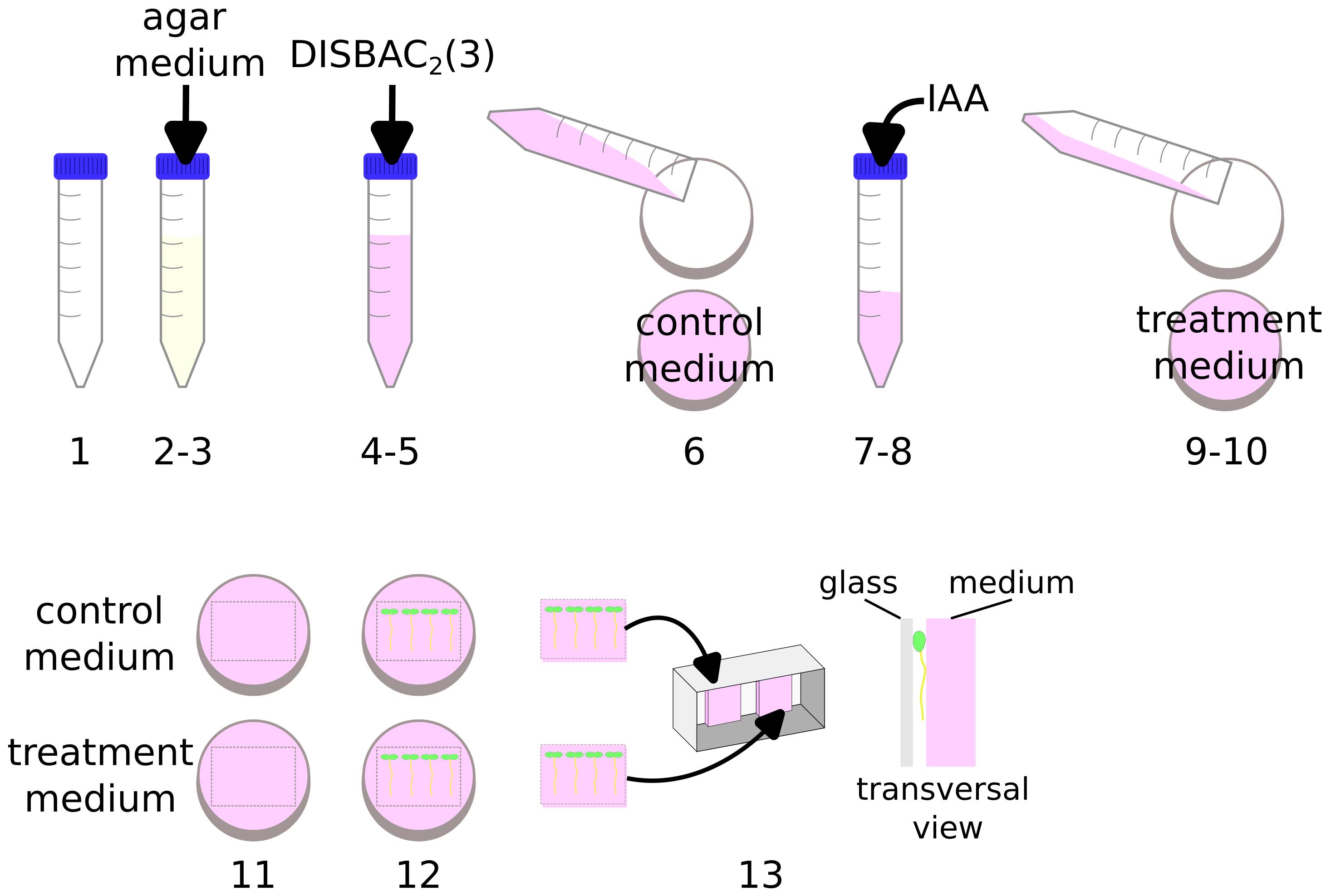
Figure 1. Preparation of solid media in microscopy chambers for agar experimentsPour 40 mL of buffered 1/2 MS pH 5.8 agar medium (see Recipes) into a 50 mL tube.
Wait a few minutes for the medium to cool down (until not burning in the hand).
Add 60 μL of DISBAC2(3) from a 2 mM aliquot to make the final concentration 3 μM.
Gently mix by inversion until the pink staining is uniform.
Pour 20 mL of this solution into a Petri dish.
Add 20 μL of IAA 100 μM into the leftover media in the tube to obtain a 100 nM final concentration (avoid agar temperature above 60 °C).
Gently mix by inversion.
Pour the IAA supplemented medium into another Petri dish.
Let the medium solidify (approximately 15 min).
In the small Petri dish, cut the agar to delimit a patch that would fit the microscopy chamber (using a thin spatula).
Transfer your seedlings to the control and treatment patches using a toothpick or tweezers to gently lift the seedlings by their cotyledons.
Transfer the patches with seedlings to the microscopy chamber (so that the seedlings are sandwiched between the agar and the chamber cover glass).
Caution: Avoid contact between both media in the chamber to prevent diffusion of IAA into the control medium.
Install the chamber on the microscope stage and let the plants recover from the transfer stress for at least 20 min (this minimum as been determined by the stage at which root elongation and fluorescence reach a stable plateau after the mechanical stress induced by the transfer).
Note: Waiting longer than 20 min does not harm the assay. During this time, you can set your microscope stage positions on your microscope software.
Once recovered, start imaging with a 515 nm excitation.
Note: Imaging settings will depend on the microscope setup and will need to be adapted by the user pre-experiment; do not change them between experiments/replicates to be able to compare control and treated plants. We routinely image plants every 10 min for 40 min to quantify root elongation as well.
Microfluidic experiments to observe fast depolarization/hyperpolarization events
A video demonstrating these steps is available in Video 2.
Video 2. Preparation of liquid media for microfluidics experimentsPrepare an IAA 100 μM solution (see Recipes).
Note: Steps are graphically represented in Figure 2 and demonstrated in Video 2.
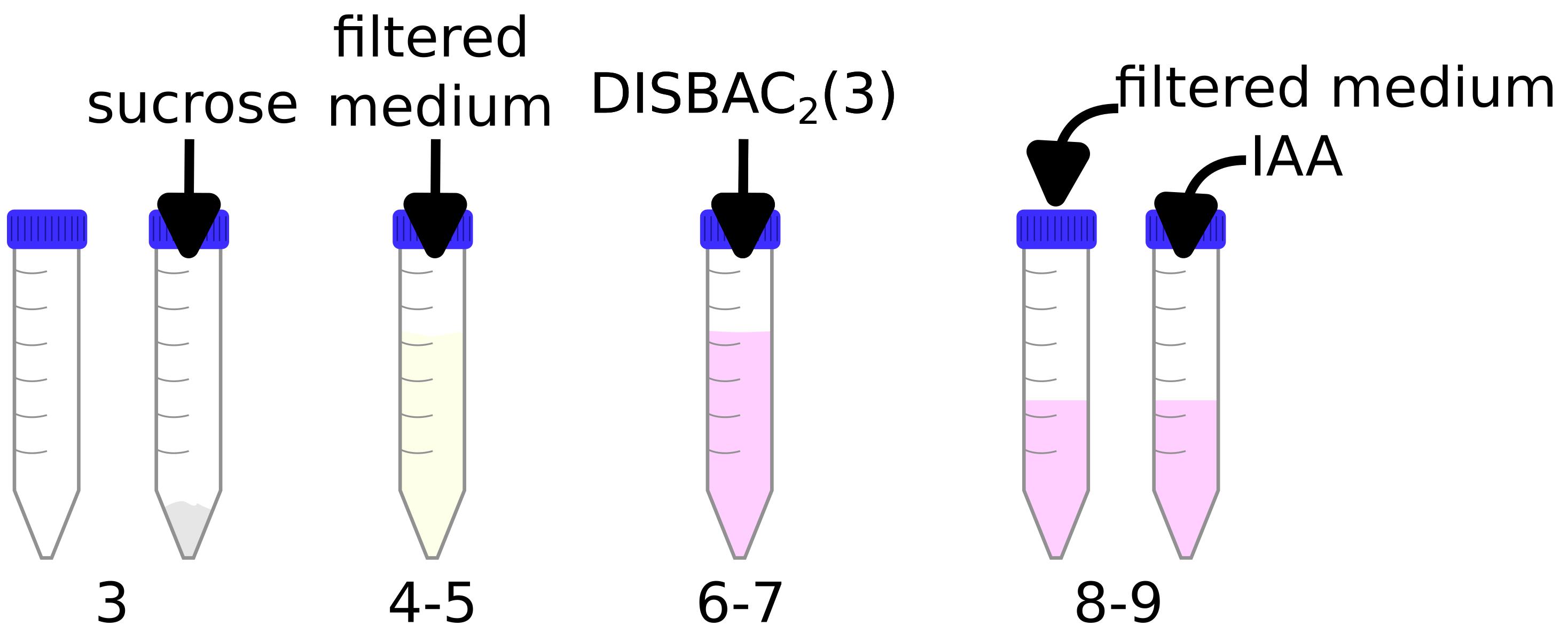
Figure 2. Preparation of liquid media for microfluidics experimentsFilter liquid buffered 1/2 MS media pH 5.8 (see Recipes) using, for example, a 0.45 μm membrane in a siphon filter.
Add 0.1 g of sucrose to an empty 15 mL tube.
Add 10 mL of the filtered media (from step C2) to the same tube.
Vortex and/or shake to fully dissolve the sucrose into the medium.
Add 10 μL of DISBAC2(3) (from a 2 mM aliquot in DMSO) to obtain a final concentration of 2 μM.
Vortex and/or shake to dissolve.
Transfer 5 mL to another 15 mL tube.
Critical: Steps C3–C8 ensure that the dye and sucrose are at the exact same concentrations in both tubes. DISBAC2(3) is used for relative measurements and thus every step counts to increase reproducibility.
Add 5 μL of buffered 1/2 MS media pH 5.8 in one tube (control tube) and 5 μL of IAA 100 μM in a second tube (treatment tube).
Continue with the procedure adapted to your microfluidic setup.
If you are using a manually closable microfluidic chip in which you directly transfer 4–5-day-old seedlings, let the seedlings recover for at least 20 min with control media flow after closing the device.
Note: During this time, you can set your microscope stage positions on your microscope software.
Start imaging with a 515 nm excitation.
After at least 5 min, switch the flow in the chip from control media to treatment media.
Note: Imaging settings depend on the microscope setup and must be adjusted by the user prior to the experiment. They must not change between experiments/replicates, to allow comparison between control and treated plants. We routinely image the plants every 30 s to observe rapid responses. For example: 5 min control condition/12 min treatment condition.
Data analysis
In this protocol, we use the imaging of the rapidly induced IAA root depolarization to showcase DISBAC2(3) as a relative membrane potential reporter. We noticed that the depolarization was the strongest above the root cap, in the root transition zone (Serre et al., 2021), a zone involved in many root responses to stresses (Baluška et al., 2010). We then carried out measuring the DISBAC2(3) fluorescence only in the root transition zone. Moreover, we focus on the interface between the cortex and the epidermis, as the dead lateral root cap cells were strongly fluorescent (open membranes for the dye to react to). The data presented here are re-analyzed images from Serre et al. (2021). Raw data can be found on Zenodo (https://zenodo.org/record/4922659). All the scripts used in this protocol can be found on the public repository https://sourceforge.net/projects/disbac2-3-data-analysis/.
Here, we describe a method to:
Quantify DISBAC2(3) fluorescence in the transition zone at a given point (agar experiment) or over time (microfluidics) using the ImageJ/Fiji software.
Quantify root elongation either as an average growth (agar experiment) or over time (microfluidics).
Normalize the microfluidics measured data in Calc or Excel.
Represent the data either with R or Python and the Seaborn plugin.
Carry non-parametric statistical analysis using the nparcomp package in R.
Note: This process would be hard to automate and, therefore, can be subjective. To avoid unconscious measuring bias, we recommend measuring the fluorescence blindly (not knowing which conditions are measured). For example, ask a colleague to change the name of your files, keeping the original names associated with the blind identifiers.
Analysis of experiments carried out in agar media
Note: Membrane potential is only measured on the first timeframe of the stack, as we are looking for a well-established response after 25 min of treatment. Root elongation is calculated as an average of 40 min of growth.
Image analysis
Fluorescence measurements:
Open one microscopy image stack in ImageJ/Fiji.
Check if scale settings are correct (Menu: Analyze > Set Scale).
Set measurements to at least Mean gray value (Menu: Analyze > Set Measurements).
Select the segmented line tool (right-click on the default straight line).
Increase line width of the segmented line tool to 20 pixels (double-click on the segmented line tool).
Display the first timeframe of the image stack.
Adjust brightness to comfortably see the root transition zone cells (shortcut Control + Shift + C or in the menu: Image > Adjust > Brightness/Contrast, Figure 3a).
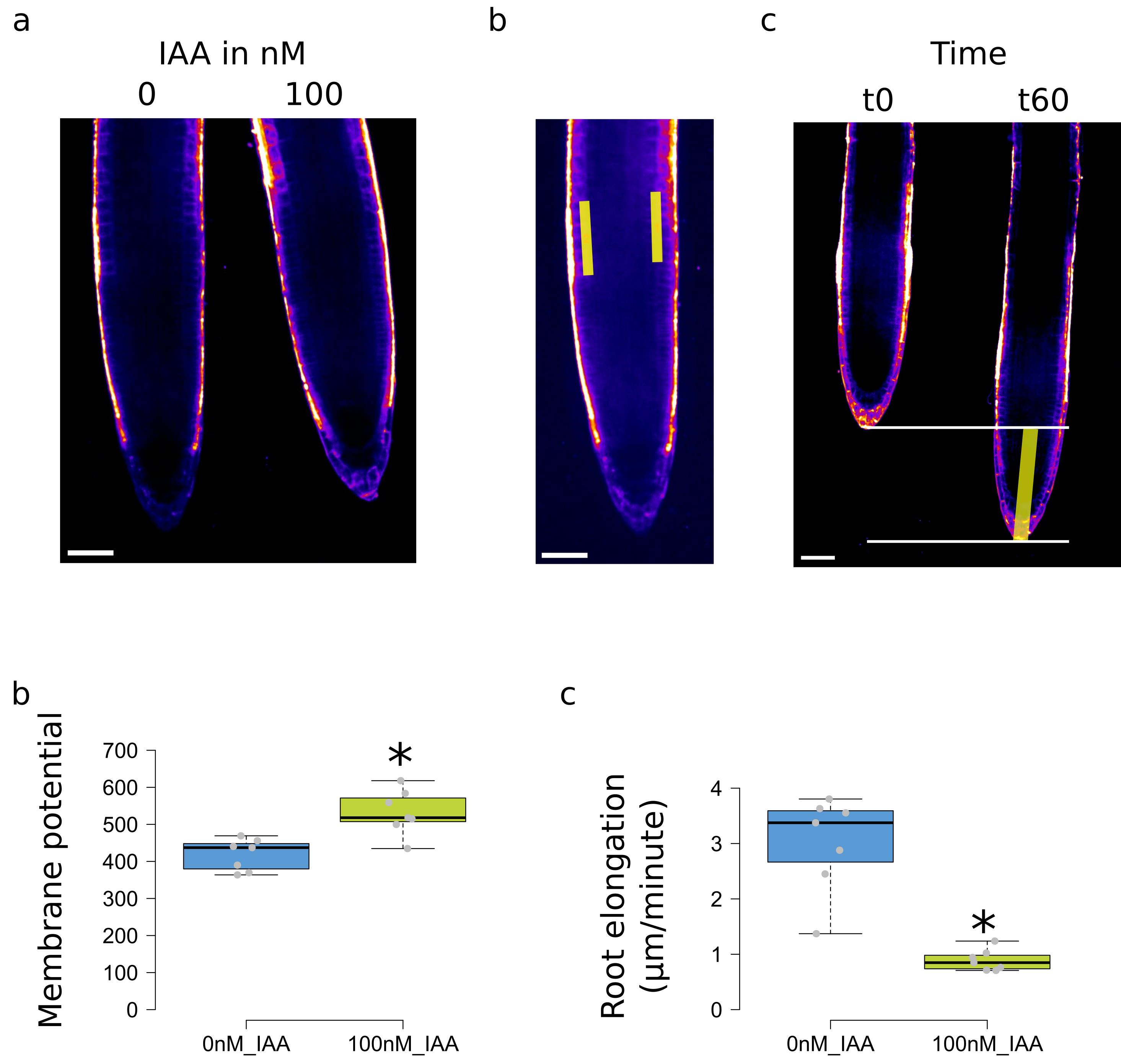
Figure 3. Measurements and plotting in solid media experiments. (a) Example of images with the gray values represented as a LUT. (b) Selection of the transition zone at the intersection between cortex and epidermis. (c) Measurements of root elongation. (d) Measured membrane potential fluorescence and (e) root elongation, values of Col-0 treatment with 0 or 100 nM IAA. Scale bar: 50 μm. For (d) and (e), the * represents a p-value < 0.05, obtained by a non-parametric Student test (npar.t.test function in the R nparcomp package).Optional: Set a LUT to display intensities as color gradients (Main bar: Lut, e.g., Green Fire blue or Fire)
Draw a segmented line on the transition zone cells on the right side of the root, centered on the membrane between root cortex and epidermis (Figure 3b, left-click to add segment, right-click to end segmented line selection).
Note: For a definition of transition zone location, see Baluška et al. (2010).
Make sure that the result table window is not open or is empty.
Measure (shortcut m or menu: Analyze > Measure).
Repeat the process from e to j for the left side of the root to measure the fluorescence (Figure 3b).
Measure (shortcut m or menu: Analyze > Measure).
Repeat process for all the roots in one condition.
Copy the measured Mean (mean fluorescence of the selection) from the result table window to an Excel spreadsheet or similar software.
Clear result table (either in result window: Results > Clear Results or by closing the window).
Root elongation measurements:
Be sure to be on the first timeframe of the image stack and that the segmented line tool is selected.
Select the extreme tip of the root (left-click).
Go to last timeframe (scroll down or image slide bar).
Select the extreme tip of the root (right-click to end selection) (Figure 3c).
Measure (shortcut m or menu: Analyze > Measure).
Repeat process for all the roots in one condition.
Copy the measured Length from the result table window to an Excel spreadsheet or similar software.
Clear result table (either in result window: Results > Clear Results or by closing the window).
Data analysis
Organize the measured data to fit Table 1 (can be in the same file, different sheets).
Table 1. Characteristics of table with measured membrane potential fluorescence and root elongation for plotting and statistics
Filename Condition Fluorescence TZ right Fluorescence TZ left Average fluorescence Root length increment (here 2 h) Root elongation in μm/min (increment/120) 0nM_root1.tif 0nM_IAA 381.715 345.623 363.669 164.622 1.37185 0nM_root2.tif 0nM_IAA 447.295 433.388 440.3415 405.015 3.375125 0nM_root3.tif 0nM_IAA 343.961 436.011 389.986 435.681 3.630675 0nM_root4.tif 0nM_IAA 392.971 481.415 437.193 456.521 3.804341667 0nM_root5.tif 0nM_IAA 488.14 423.733 455.9365 426.512 3.554266667 0nM_root6.tif 0nM_IAA 371.998 367.106 369.552 345.512 2.879266667 0nM_root7.tif 0nM_IAA 546.02 392.141 469.0805 294.079 2.450658333 100nM_root1.tif 100nM_IAA 490.262 627.423 558.8425 122.673 1.022275 100nM_root2.tif 100nM_IAA 585.199 444.535 514.867 84.957 0.707975 100nM_root3.tif 100nM_IAA 538.38 497.549 517.9645 91.505 0.762541667 100nM_root4.tif 100nM_IAA 414.893 454.586 434.7395 101.832 0.8486 100nM_root5.tif 100nM_IAA 501.4 498.181 499.7905 148.582 1.238183333 100nM_root6.tif 100nM_IAA 552.743 614.447 583.595 85.581 0.713175 100nM_root7.tif 100nM_IAA 517.162 718.587 617.8745 113.049 0.942075 Open R software (or R Studio IDE).
Open the R script supplemented. For comparisons and plotting of two conditions, use “R_script-agar_2conditionsgenotypes.R.” For more than two conditions, use: “R_script-agar_3andplusconditionsgenotypes.R.”
Follow the script comments to modify the script to your conditions.
Execute Script.
Save boxplot as svg (for possible aesthetical modifications in Inkscape, Figure 3d–3e).
Save output of the statistics by copy and pasting into a notepad.
Analysis of experiments carried out in microfluidics
In microfluidics experiments, membrane potential is measured over time to have access to the dynamic response after treatment. We also propose a way to measure root elongation rates over time.
Image analysis for one condition (e.g., control to 100 nM IAA switch)
Determining the timeframe associated with the treatment arrival:
In our imaging conditions, we observed a small drop in background fluorescence during medium switches. This allowed us to determine which timeframe should be considered as time zero for the treatment. This prevents the use of fluorescent tracers such as Fluorescein dextran (see Recipes if a tracer is needed in your experimental conditions).
Open one microscopy image stack in ImageJ/Fiji.
Check if scale settings are correct (Menu: Analyze > Set Scale).
Set measurements to at least Mean gray value (Menu: Analyze > Set Measurements).
Select a region of interest (ROI) in the background as far as possible from the root (Figure 4a).
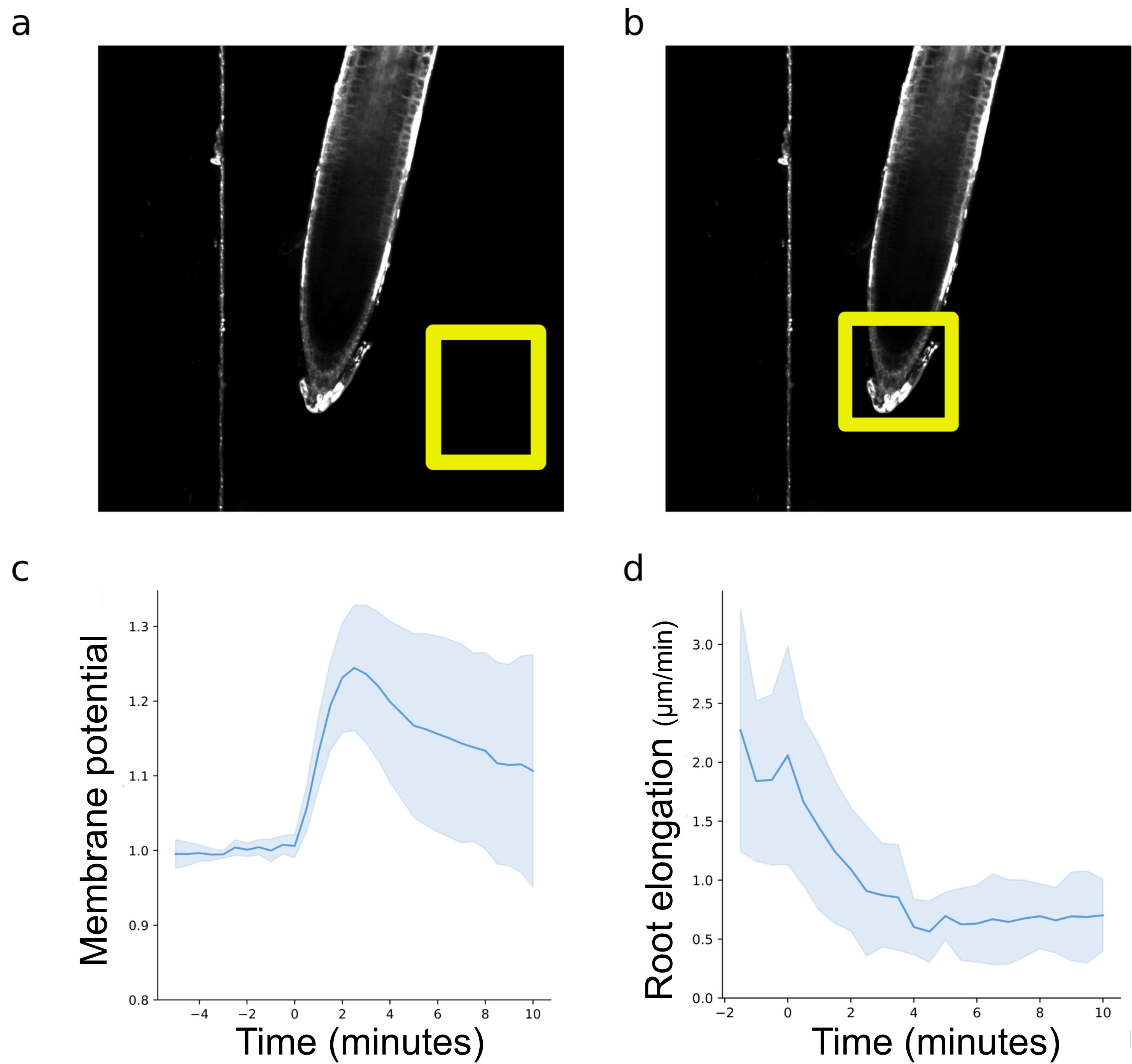
Figure 4. Measurements and plotting microfluidic experiments. (a) Selection of a background region of interest to determine the treatment arrival. (b) Rectangular selection of the root tip to determine root elongation rates over time. (c) Measured and normalized DISBAC2(3) fluorescence reflecting the membrane potential and (d) root elongation; values of Col-0 observed 5 min in control and then 10 min with IAA 100 nM. For (c) and (d), negative values represent the root being exposed to the control medium, and positive values represent the root being exposed to the treatment medium.Add this ROI to the ROI manager (Shortcut Ctrl + t or Analyze/Tools/ROI Manager).
Make sure that the result table window is not open or is empty.
Select the added selection in the ROI manager and click on more >> Multi Measure. A window will pop up; ensure that the options Measure all xx slices and One row per slice are ticked.
Then, click OK.
Copy and paste the results from the result table into an Excel table.
Note: The arrival of the treatment is marked by either a clear drop in background fluorescence or a small but sharp increase, followed by a drop in background fluorescence. If you have trouble determining the treatment arrival in your conditions, see Recipes for fluorescent tracer.
Stabilization of the root on the image stack:
Select the segmented line tool (right-click on the default straight line).
Increase line width of the segmented line tool to 20 pixels (double-click on the segmented line tool).
Display the first timeframe of the image stack.
Adjust brightness to comfortably see the root transition zone cells (shortcut Control + Shift + C or in the menu: Image > Adjust > Brightness/Contrast).
Optional: Set a LUT to display intensities as color gradients (Main bar: Lut, e.g., Green Fire blue or Fire).
Draw a segmented line on the transition zone cells on the right side of the root, centered on the membrane between root cortex and epidermis (as in Figure 3b, left-click to add segment, right-click to end segmented line selection).
Start the Correct 3D drift plugin (Plugins/Registration/Correct 3D drift).
In the window, select the channel for registration (the fluorescence channel works well, but we also had great results with brightfield), and then click OK.
Add your transition zone ROIs (left and right sides) to the registered stack into the ROI Manager and check that the selection is always on the transition zone over time.
Note: If the selections are not stable over time, try the registration with the Sub pixel drift correction, and/or use the other side of the root and/or register on one side and then the other.
Make sure that the result table window is not open or is empty.
Once the ROIs are stable over time, click more >>/Multi measure in the ROI Manager window.
Copy and paste the results from the result table into an Excel table (only keeping the Mean1 and Mean2 columns.
Repeat the process of 1a and 1b for all your image stacks in control and treatment condition(s).
Root elongation measurements:
Go back to the original image stack (not registered).
Make a rectangular selection on the root tip (Figure 4b).
Open the Correct 3D drift plugin (Plugins/Registration/Correct 3D drift).
In the window, select the channel for registration and then tick Only compute drift vectors?
Rename the measure text file with the name of your raw image stack (or desired name) and save it.
Data analysis
Fluorescence analysis:
Organize the measured data to fit Table 2 (the name of the column Time is essential for the script to recognize the column).
Open the python script fluorescence_analysis.py in the Spyder IDE.
Modify the user inputs at the beginning of the code and run.
The script will import, normalize, and plot your data (Figure 4c).
Note: The normalization process is explained in the Materials and Methods of Serre et al. (2021).
Table 2. Characteristics of table with measured membrane potential fluorescence for analysis. Negative times represent the control window, zero is the timeframe of the media switch, and positive times represent the treatment window.
Time (min) Root1 Root2 Root3 Root4 Root5 Root6 Root7 Root8 -5 408.908372 389.499513 392.495975 327.607 411.428 395.879762 403.292463 411.977079 -4.5 405.668564 386.243762 393.183715 327.672 413.428 397.335688 404.113862 413.522185 -4 403.082014 386.306109 392.140659 332.045 413.523 395.057337 404.527451 417.715058 -3.5 396.392234 385.716733 390.918841 333.657 414.2265 396.265252 402.175133 418.270171 -3 395.523104 380.711613 392.716895 335.763 416.6785 396.086036 401.628771 419.469708 -2.5 397.419366 381.983792 396.580456 339.207 420.0695 396.374816 412.618216 423.596701 -2 392.097153 381.825249 399.140425 342.854 418.4595 396.809199 405.392976 420.864414 -1.5 399.883876 379.197157 401.737308 347.443 418.183 399.659632 399.678631 421.315916 -1 396.454276 377.647971 403.093227 347.078 418.119 399.218287 392.094359 419.257999 -0.5 398.013425 378.172317 403.254221 349.409 418.368 402.997758 404.306832 423.040022 0 400.452519 382.279517 407.598904 349.563 418.121 397.010205 394.462017 422.650659 0.5 419.649339 390.901924 441.873124 358.037 434.2055 415.260263 439.403187 431.782716 1 442.17854 416.22474 475.150674 380.477 463.097 442.370851 490.670599 458.766988 … … … … … … … … … 9.5 398.475274 452.643626 466.316994 405.541 491.053 528.389269 360.38102 406.706359 10 399.328873 452.295109 467.085197 395.029 486.823 534.563718 344.475839 403.269758
Root elongation analysis:
Regroup all the shifts text files into a dedicated folder.
Retrieve scale (in pixels/μm) from one of your stacks of images (Fiji > Analyze > Set Scale).
Open the python script elongation_compilation.py in the Spyder IDE.
Modify the user inputs at the beginning of the code and run the script to create a table with all your root elongation rates calculated in μm/min at each time point.
Note: This script takes the x and y coordinates shifts over time and 1) calculates the distance between the coordinates time +1 and time +0, 2) transform those coordinates in μm using the user scale, and 3) divides the data by the duration of the timeframes in minutes to obtain μm/min.
Open the saved table into an Excel table and manually add the Time (name is essential) column as a first column to resemble Table 2.
Open the python script elongation_plotting.py in the Spyder IDE.
Modify the user inputs at the beginning of the code and run the script to create the line plot (Figure 4d).
Note: For plotting more than two conditions in microfluidics (e.g., control to 100 nM IAA and control to 1,000 nM IAA), the scripts fluorescence_analysis.py and elongation_compilation.py should be run on the individual conditions. We then provide another python script: plotting_fluo_elongation_2andmore.py.
Validation of protocol
The development and validation of this method is described in detail in Serre et al. (2021).
Notes
Reproducibility
The DISBAC2(3) staining method can be very reproducible if the user 1) respects the dye dilution steps and 2) minimizes mechanical stress during transfer and 3) the recovery time before imaging.
Particularities we observed
Dead cells shine considerably more than living cells, as the dye is able to freely stain membranes inside and outside (e.g., dead root cap cells).
The outer cells (epidermis/cortex) fluoresce more, but observations by multi-photons microscopy revealed that the dye actually penetrates the whole root (Serre et al., 2021).
DISBAC2(3) tends to stick to microfluidics tubing (such as Tygon or PTFE), especially when the flow is stopped. We observed lower fluorescence intensities switching from one control medium to another control medium. This emphasizes the need for proper controls and the relative aspect of this method.
Rapidity of response
Depolarizations can be very fast and transient and might not be visible after a few minutes [e.g., agar imaging with low concentration of IAA (< 100 nM)]. The IAA-induced depolarization is statistically still visible in agar after 25 min at strong concentrations above 100 nM.
Vertical microscopy
If using a vertical microscope, always keep your seedlings oriented toward the gravity (while growing, moving the plate, on the bench, during transfer to agar patches, and in the microscopy chamber). This will prevent auxin fluxes from being triggered, which could bias measurements.
Recipes
DISBAC2(3) master stock [for a 100 mg bottle of DISBAC2(3) powder]
Add 2.290 mL of DMSO directly into the bottle (final concentration of 100 mM).
Vortex until fully dissolved.
Keep at -20 °C.
DISBAC2(3) working aliquots
Add 392 μL of DMSO into a 1.5 mL tube.
Add 8 μL of DISBAC2(3) master stock at 100 mM (Recipe 1) to obtain a 2 mM final concentration.
Vortex.
Aliquot in 20 μL in 500 μL tubes.
Keep at -20 °C.
70% ethanol (approximately) prepared from 96% ethanol
Pour 175 mL of 96% ethanol into a graduated cylinder.
Pour distilled water up to 250 mL.
Keep at room temperature.
500 mL of buffered liquid 1/2 MS
In a 500 mL beaker, weigh and add:
1.1 g of Murashige and Skoog mix
0.3 g of MES hydrate
Add approximately 450 mL of Milli-Q or distilled water to the beaker.
Add magnetic rod and mix with a magnetic mixer until all powders are dissolved.
Raise pH to 5.8 with 1 M KOH using a pH meter.
Remove magnetic rod and transfer to a 500 mL graduated cylinder.
Add water up to 500 mL.
Filter in a 0.5 L glass bottle using a siphon filter or a syringe filter.
Keep at room temperature.
500 mL of buffered solid 1/2 MS
In a 500 mL beaker, weigh and add:
1.1 g of Murashige and Skoog mix
5 g of sucrose (final concentration of 1% m/v)
0.3 g of MES hydrate
Add approximately 450 mL of Milli-Q or distilled water to the beaker.
Add magnetic rod and mix with a magnetic mixer until all powders are dissolved.
Raise pH to 5.8 with 1 M KOH using a pH meter.
Remove magnetic rod and transfer to a 500 mL graduated cylinder.
Add water up to 500 mL.
Add 4 g of plant agar to a 0.5 L glass bottle.
Add the medium from step 5e.
Autoclave with cap half unscrewed.
Keep bottle in a 50/60 °C incubator to keep it liquid, use directly after autoclave, or let solidify and dissolve agar in microwave before use (up to two times).
IAA 10 mM stock
Let the IAA powder bottle come to room temperature (30 min on the bench).
Using a precision scale, weigh 17.518 mg of powder and add to a 15 mL tube.
Add 10 mL of 70 % ethanol (Recipe 3) in the 15 mL tube (final concentration of 10 mM).
Vortex until dissolved.
Cover the tube with aluminum foil and store at -20 °C for up to one month.
IAA 100 μM solution
Add 990 μL of liquid 1/2 MS (Recipe 4) into a 1.5 mL tube.
Add 10 μL of IAA 10 mM (Recipe 6) to obtain a final concentration of 100 μM.
Vortex.
Discard after one day at room temperature.
Fluorescent tracer (to follow treatment arrival in microfluidics)
Weigh 10 mg of Fluorescein Dextran 10 K MW into a 1.5 mL tube.
Add 1 mL of distilled water for a 10 mg/mL final concentration.
Vortex until fully dissolved.
Add 0.6 μL per mL of control liquid medium.
Add 0.3 μL per mL of treatment liquid medium.
The fluorescent tracer is visible with a 515 and 488 nm excitation source.
Caution: We advise to alternate the two concentrations in the control/treatment media to be sure that the observed effects are not from the tracer. It is important to add the tracer in two different concentrations in both media to minimize potential effects of the dye, as minimal but visible effects on root elongation can be observed.
Acknowledgments
This work was supported by the European Research Council (grant no. 803048). This protocol is a detailed version of the material and methods and reproduces results published in Serre et al. (2021).
Competing interests
The authors declare no competing interests.
References
- Baluška, F., Mancuso, S., Volkmann, D. and Barlow, P. W. (2010). Root apex transition zone: a signalling–response nexus in the root. Trends Plant Sci. 15(7): 402–408.
- Cuin, T. A., Betts, S. A., Chalmandrier, R. and Shabala, S. (2008). A root’s ability to retain K+ correlates with salt tolerance in wheat. J. Exp. Bot. 59(10): 2697–2706.
- Dindas, J., Becker, D., Roelfsema, M. R. G., Scherzer, S., Bennett, M. and Hedrich, R. (2020). Pitfalls in auxin pharmacology. New Phytol. 227(2): 286–292.
- Dindas, J., Scherzer, S., Roelfsema, M. R. G., von Meyer, K., Müller, H. M., Al-Rasheid, K. A. S., Palme, K., Dietrich, P., Becker, D., Bennett, M. J., et al. (2018). AUX1-mediated root hair auxin influx governs SCFTIR1/AFB-type Ca2+ signaling. Nat. Commun. 9(1): e1038/s41467-018-03582-5.
- Fendrych, M., Akhmanova, M., Merrin, J., Glanc, M., Hagihara, S., Takahashi, K., Uchida, N., Torii, K. U. and Friml, J. (2018). Rapid and reversible root growth inhibition by TIR1 auxin signalling. Nat. Plants 4: 453–459.
- Grossmann, G., Guo, W.-J., Ehrhardt, D. W., Frommer, W. B., Sit, R. V., Quake, S. R. and Meier, M. (2011). The RootChip: An Integrated Microfluidic Chip for Plant Science. Plant Cell 23(12): 4234–4240.
- Konietschke, F., Placzek, M., Schaarschmidt, F. and Hothorn, L. A. (2015). nparcomp: An R Software Package for Nonparametric Multiple Comparisons and Simultaneous Confidence Intervals. J. Stat. Softw. 64(9): 1–17.
- Li, L., Verstraeten, I., Roosjen, M., Takahashi, K., Rodriguez, L., Merrin, J., Chen, J., Shabala, L., Smet, W., Ren, H., et al. (2021). Cell surface and intracellular auxin signalling for H+ fluxes in root growth. Nature 599(7884): 273–277.
- Lindsey, B. E., Rivero, L., Calhoun, C. S., Grotewold, E. and Brkljacic, J. (2017). Standardized Method for High-throughput Sterilization of Arabidopsis Seeds. J. Vis. Exp. (128): e56587.
- Mudrilov, M., Ladeynova, M., Grinberg, M., Balalaeva, I. and Vodeneev, V. (2021). Electrical Signaling of Plants under Abiotic Stressors: Transmission of Stimulus-Specific Information. Int. J. Mol. Sci. 22(19): 10715.
- Paponov, I. A., Dindas, J., Król, E., Friz, T., Budnyk, V., Teale, W., Paponov, M., Hedrich, R. and Palme, K. (2019). Auxin-Induced Plasma Membrane Depolarization Is Regulated by Auxin Transport and Not by AUXIN BINDING PROTEIN1. Front. Plant Sci. 9: e01953.
- Qi, L., Kwiatkowski, M., Chen, H., Hoermayer, L., Sinclair, S., Zou, M., del Genio, C. I., Kubeš, M. F., Napier, R., Jaworski, K., et al. (2022). Adenylate cyclase activity of TIR1/AFB auxin receptors in plants. Nature 611(7934): 133–138.
- Ragel, P., Raddatz, N., Leidi, E. O., Quintero, F. J. and Pardo, J. M. (2019). Regulation of K+ Nutrition in Plants. Front. Plant Sci. 10: e00281.
- Schindelin, J., Arganda-Carreras, I., Frise, E., Kaynig, V., Longair, M., Pietzsch, T., Preibisch, S., Rueden, C., Saalfeld, S., Schmid, B., et al. (2012). Fiji: an open-source platform for biological-image analysis.Nat Methods 9(7): 676-682.
- Roosjen, M., Kuhn, A., Mutte, S. K., Boeren, S., Krupar, P., Koehorst, J., Fendrych, M., Friml, J. and Weijers, D. (2022). An ultra-fast, proteome-wide response to the plant hormone auxin. Plant Biology.: e517949.
- Shabala, L., Cuin, T. A., Newman, I. A. and Shabala, S. (2005). Salinity-induced ion flux patterns from the excised roots of Arabidopsis sos mutants. Planta 222(6): 1041–1050.
- Serre, N. B. C., Kralík, D., Yun, P., Slouka, Z., Shabala, S. and Fendrych, M. (2021). AFB1 controls rapid auxin signalling through membrane depolarization in Arabidopsis thaliana root. Nat. Plants 7(9): 1229–1238.
- Sze, H. (1985). H+-Translocating ATPases: Advances Using Membrane Vesicles. Annu. Rev. Plant Physiol. 36(1): 175–208.
- Sze, H., Li, X. and Palmgren, M. G. (1999). Energization of Plant Cell Membranes by H+ -Pumping ATPases: Regulation and Biosynthesis. Plant Cell 11(4): 677–689.
- Tretyn, A., Wagner, G. and Felle, H. H. (1991). Signal Transduction in Sinapis alba Root Hairs: Auxins as External Messengers. J. Plant Physiol. 139(2): 187–193.
- Tyerman, S. D. and Schachtman, D. P. (1992). The role of ion channels in plant nutrition and prospects for their genetic manipulation. Plant Soil 146: 137–144.
- von Wangenheim, D., Hauschild, R., Fendrych, M., Barone, V., Benková, E. and Friml, J. (2017). Live tracking of moving samples in confocal microscopy for vertically grown roots. eLife 6: e26792.
- Yanagisawa, N., Kozgunova, E., Grossmann, G., Geitmann, A. and Higashiyama, T. (2021). Microfluidics-Based Bioassays and Imaging of Plant Cells. Plant Cell Physiol. 62(8): 1239–1250.
Article Information
Copyright
© 2023 The Author(s); This is an open access article under the CC BY-NC license (https://creativecommons.org/licenses/by-nc/4.0/).
How to cite
Dubey, S. M., Fendrych, M. and Serre, N. B. C. (2023). Relative Membrane Potential Measurements Using DISBAC2(3) Fluorescence in Arabidopsis thaliana Primary Roots. Bio-protocol 13(14): e4778. DOI: 10.21769/BioProtoc.4778.
Category
Plant Science > Plant cell biology > Cell imaging
Plant Science > Plant developmental biology > General
Cell Biology > Cell imaging > Live-cell imaging
Do you have any questions about this protocol?
Post your question to gather feedback from the community. We will also invite the authors of this article to respond.